In this section we propose lower and upper bounds on the eccentricity, a strategy that accommodates the second type of speedup. We will also outline a pruning strategy that helps to reduce both the number of nodes that have to be investigated, as well as the size of the graph, realizing both of the two speedups listed above.
4.1. Eccentricity Bounds
We propose to use the following bounds on the eccentricity of all nodes , when the eccentricity of one node has been computed:
Observation 1 For nodes we have .
The upper bound can be understood as follows: if node w is at distance from node v, it can always employ v to get to every other node in steps. To get to node v, exactly steps are needed, totalling steps to get to any other node. The first part of the lower bound () can be derived in the same way, by interchanging v and w in the previous statement. The second part of the lower bound, itself, simply states that the eccentricity of w is at least equal to some found distance to w.
The bounds from Observation 1 were suggested in [
6] as a way to determine which nodes could contribute to a graph’s diameter. We extend the method proposed in that paper by using these bounds to compute the full eccentricity distribution of the graph. The approach is outlined in Algorithm 2.
First, the candidate set W and the lower and upper eccentricity bounds are initialized (lines 3–8). In the main loop of the algorithm, a node v is repeatedly selected (line 10) from W, its eccentricity is determined (line 11), and finally all candidate nodes are updated (line 12–19) according to Observation 1. Note that the value of which is used in the updating process does not have to be computed, as it is already known because it was calculated for all w during the computation of the eccentricity of v. If the lower and upper eccentricity bounds for a node have become equal, then the eccentricity of that node has been derived and it is removed from W (lines 15–18). Algorithm 2 returns a vector containing the exact eccentricity value of each node. Counting the number of occurrences of each eccentricity value results in the eccentricity distribution.
An overview of possible selection strategies for the function S
electF
rom can be found in [
6]. In line with results presented in that work, we found that when determining the eccentricity distribution, interchanging the selection of a node with a small lower bound and a node with a large upper bound, breaking ties by taking a node with the highest degree, yielded by far the best results. As described in [
6], examples of graphs in which this algorithm would definitely not work are complete graphs and circle-shaped graphs. However, most real-world graphs adhere to the small world property [
17], and in these graphs the eccentricity distribution is sufficiently diverse so that the eccentricity lower and upper bounds can effectively be utilized.
| Algorithm 2 BoundingEccentricities |
1: Input: Graph G(V, E)
2: Output: Vector ε, containing ε(v) for all v ∈ V
3: W ← V
4: for w ∈ W do
5:    ε[w] ← 0   εL[w] ← −∞   εU[w] ← +∞
6: end for
7: while W ≠ Ø do
8:    v ← SelectFrom(W)
9:    ε[v] ← Eccentricities(v)
10:   for w ∈ W do
11:       εL[w] ← max(εL[w], max(ε[v] − d(v,w), d(v,w)))
12:       εU[w] ← min(εU[w], ε[v] + d(v,w))
13:       if (εL[w] = εU[w]) then
14:            ε[w] ← εL[w]
15:            W ← W − {w}
16:        end if
17:    end for
18: end while
19: return ε
|
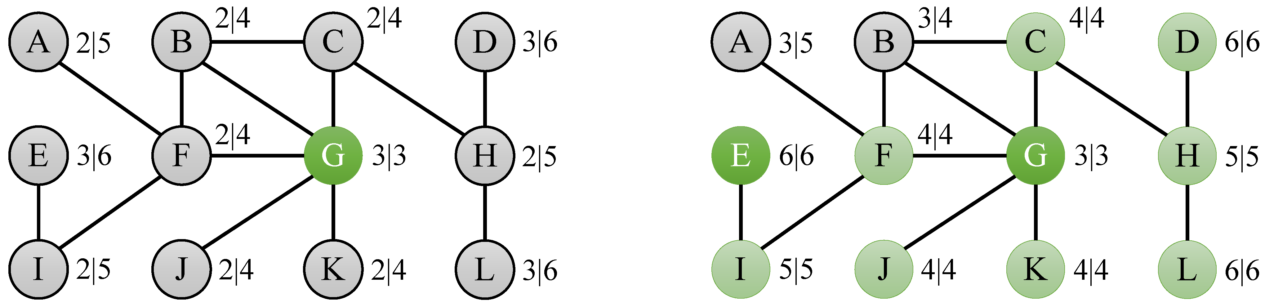
Figure 3.
Eccentricity bounds of the toy graph in
Figure 2 after subsequently computing the eccentricity of node G (left) and node E (right).
Figure 3.
Eccentricity bounds of the toy graph in
Figure 2 after subsequently computing the eccentricity of node G (left) and node E (right).
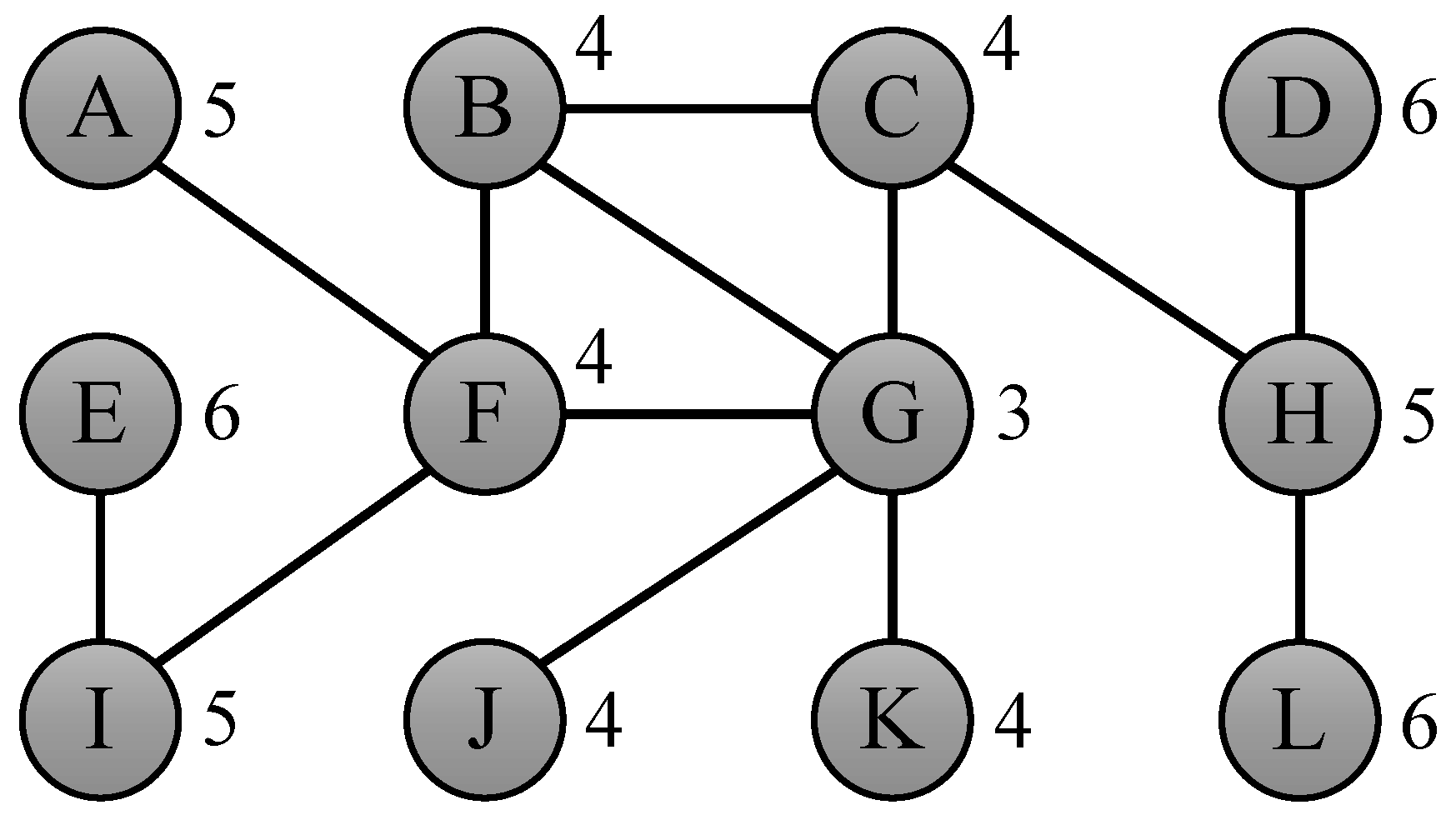
As an example of the usefulness of the bounds suggested in this section, consider the problem of determining the eccentricities of the nodes of the toy graph from
Figure 2. If we compute the eccentricity of node G, which is 3, then we can derive bounds
for the nodes at distance 1 (B, C, F, J and K),
for the nodes at distance 2 (A, H and I) and
for the nodes at distance 3 (D, E and L), as depicted by the left graph in
Figure 3. If we then compute the eccentricity of node E, which is 6, we derive bounds
for node I,
for node F,
for nodes A, B and G,
for nodes C, J and K,
for node K, and
for nodes D and L. If we combine these bounds for each of the nodes, then we find that lower and upper bounds for a large number of nodes have become equal:
for C, F, J and K,
for H and I, and
for D and L, as shown by the right graph in
Figure 3. Finally, computing the eccentricity of nodes A and B results in a total of 4 real eccentricity calculations to compute the complete eccentricity distribution, which is a speedup of 3 compared to the naive algorithm, which would simply compute the eccentricity for all 12 nodes in the graph.
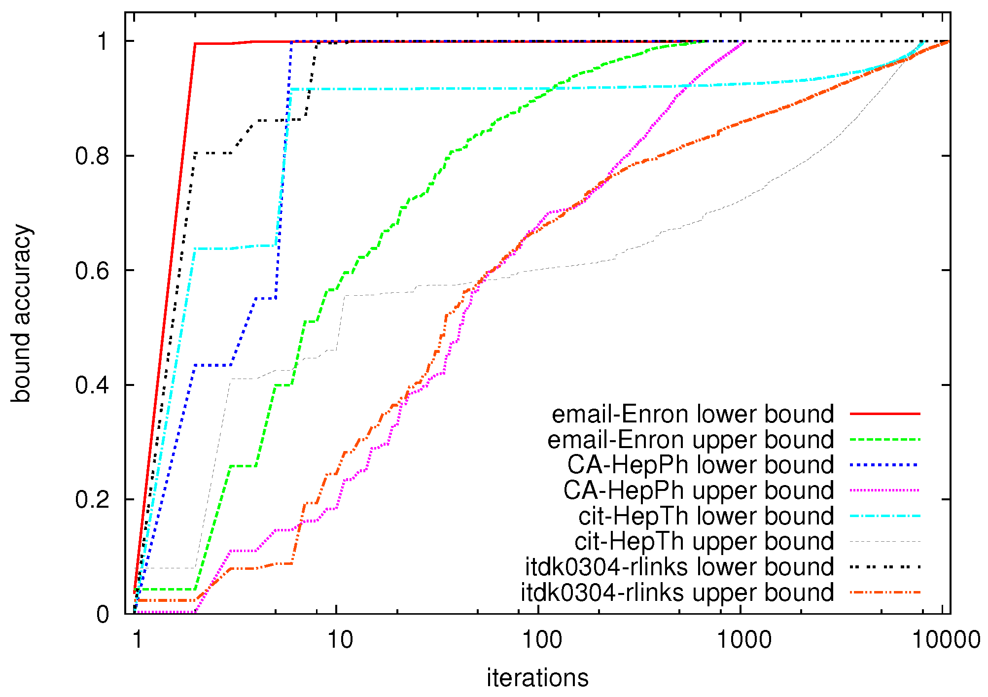
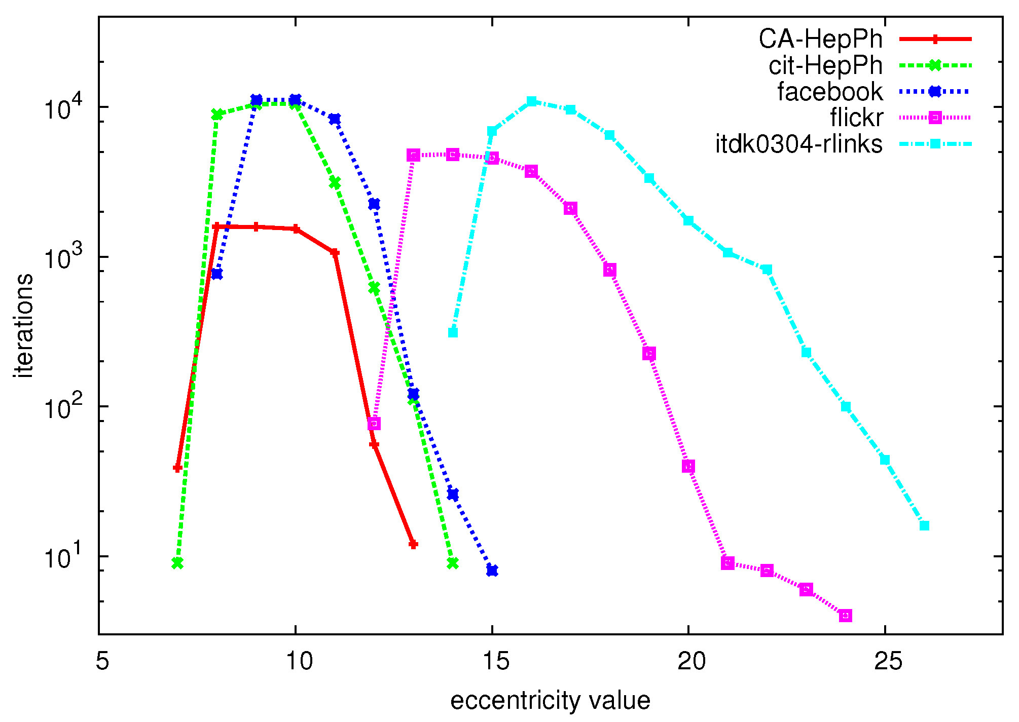
To give a first idea of the performance of the algorithm on large graphs,
Figure 4 shows the number of iterations (vertical axis) that are needed to compute the eccentricity of all nodes with given eccentricity value (horizontal axis) for a number of large graphs (for a description of the datasets, see
Section 6.1). We can clearly see that especially for the extreme values of the eccentricity distribution, very few iterations are needed to compute all of these eccentricity values, whereas many more iterations are needed to derive the values in between the extreme values.
Figure 4.
Eccentricity values (horizontal axis) vs. number of iterations to compute the eccentricity of all nodes with this eccentricity value (vertical axis).
Figure 4.
Eccentricity values (horizontal axis) vs. number of iterations to compute the eccentricity of all nodes with this eccentricity value (vertical axis).
4.2. Pruning
In this subsection we introduce a pruning strategy, which is based on the following observation:
Observation 2 Assume that . For a given , all nodes with have .
Node w is only connected to node v, and will thus need node v to reach every other node in the graph. If node v can do this in steps, then node w can do this is in exactly steps. The restriction on the graph size excludes the case in which the graph consists of v and w only.
All interesting real-world graphs have more than two nodes, making Observation 2 applicable in our algorithm, as suggested in [
6]. For every node
we can determine if
v has neighbors
w with
. If so, we can prune all but one of these neighbors, as their eccentricity will be equal, because they all employ
v to get to any other node. In
Figure 2, node G has two neighbors with degree one, namely J and K. According to Observation 2, the eccentricity values of these two nodes are equal to
J
K
G
. The same argument holds for nodes D and L with respect to node H. We expect that Observation 2 can be applied quite often, as many of the graphs that are nowadays studied have a power law degree distribution [
18], meaning that there are many nodes with a very low degree (such as a degree of 1).
Observation 2 can be beneficial to our algorithm in two ways. First, when computing the eccentricity of a single node, the pruned nodes can be ignored in the shortest path algorithm. Second, when the eccentricity of a node v has been computed (line 11 of Algorithm 2), and this node has adjacent nodes w with , then the eccentricity of these nodes w can be set to .


