1. Introduction
Hyperspectral remote sensing obtains information from the visible and the near-infrared spectrum of reflected light. Agriculture, mineralogy, physics, surveillance, and so on are just some examples of applications of the hyperspectral images.
This technology is continually in evolution and it is gradually becoming available to the public.
In military and civilian applications the remote acquisition of high definition electro-optic images has been increasingly used. Moreover, these air-borne and space-borne acquired data are used to recognize objects and to classify materials on the surface of the earth.
It is possible to recognize the materials pictured in the acquired three-dimensional data by analysis of the spectrum of the reflected light.
NASA and other organizations have catalogues of various minerals and their spectral signatures. The new technologies for hyperspectral remote sensing acquisition allow the recording of a large number of spectral bands, over the visible and reflected infrared region. The obtained spectral resolution is sufficient for an accurate characterization of the spectral reflectance curve of a given spatial area.
Higher resolution sensors will be available in the near future that will permit to increase the number of spectral bands. In fact, the increase in the number of bands, i.e., spectral resolution, shall make possible a more sophisticated analysis of the target region.
The volume of data generated daily by each sensor is in the order of many gigabytes and this brings an important need for efficient compression.
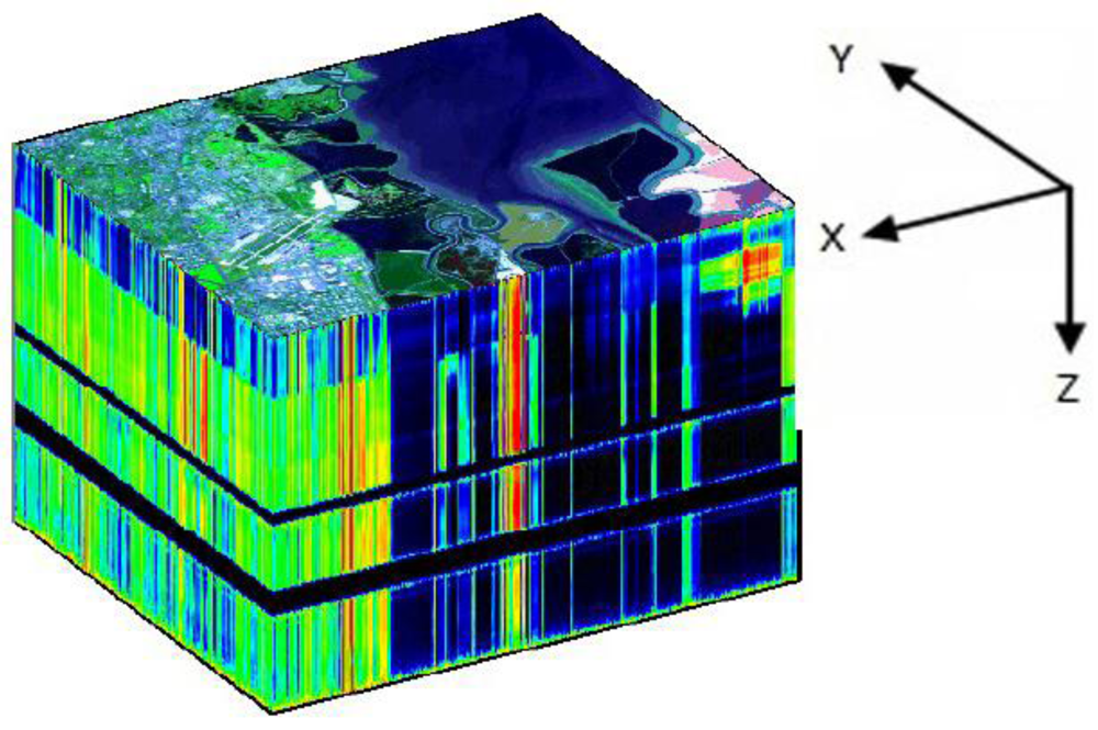
Figure 1 shows a sample of data cube for a hyperspectral image. The X-axis indicates the columns, the Y-axis indicates the rows and the Z-axis indicates the bands.
Figure 1.
Example of data cube for a hyperspectral image.
Figure 1.
Example of data cube for a hyperspectral image.
We focus our attention on visualization, band ordering and compression of hyperspectral imagery.
Section 2 discusses the visualization of hyperspectral images. We introduce a tool for hyperspectral image visualization and present an implementation on Google Android OS.
Section 3 addresses the compression problem by considering an efficient and low complexity algorithm for lossless compression of three-dimensional hyperspectral data, called the Spectral oriented Least SQuares (SLSQ) algorithm.
Section 4 presents an efficient band ordering based on two metrics: Pearson’s correlation and Bhattacharyya distances, which can lead to improvements to the SLSQ algorithm.
Section 5 reports the experimental results achieved by a Java-based implementation respectively without band ordering, with Pearson’s correlation-based and with Bhattacharyya distance-based band ordering.
Section 6 presents our conclusions and discusses future works.
2. Visualization of Hyperspectral Images
A hyperspectral image is a collection of information derived from the electromagnetic spectrum of the observed area. Unlike the human eye that can only see visible light, i.e., the wavelengths between 380 and 760 nanometers (nm), the hyperspectral images reveal the frequencies of ultraviolet and infrared rays.
Each material has an unambiguous fingerprint in the electromagnetic spectrum (spectral signatures). The spectral signature allows the identification of different types of materials.
There is a wide range of real life applications where hyperspectral remote sensing plays a very important role. For example, in geological applications the ability of hyperspectral images to identify the various types of minerals makes them an ideal tool for oil and mining industries, and hyperspectral remote sensing is used to search for minerals and oil. Other important fields of application are ecology, surveillance, historical research, archeology, etc.
The hyperspectral sensor for the Airborne Visible/Infrared Imaging Spectrometer (AVIRIS) [
8] format measures the spectrum from an area of 400 up to 2500 nm, with a nominal 10 nm sampling. This generates 224 narrows spectral bands. The resulting hyperspectral data allows an analysis of the composition of materials by using spectrographic analysis that defines how materials react to solar radiation.
The AVIRIS system measures and records the power level of the radiance of the instrument.
In the rest of this paper we have tested our approach on six hyperspectral images provided freely by NASA JPL: Cuprite, Lunar Lake, Moffett Field, Jasper Ridge, Low Altitude and Yellowstone.
The Cuprite hyperspectral image was collected from the site of Cuprite mining district, located in Nevada (USA).
Lunar Lake was acquired from the site of the Lunar Lake in Nye County, Nevada, USA.
Moffett Field was captured from Moffett Federal Airfield ([
9]), a civil-military airport in California (USA) between Mountain View and Sunnyvale.
The
Jasper Ridge hyperspectral image covers a portion of the Jasper Ridge Biological Preserve ([
10]), located in California (USA).
The Low Altitude hyperspectral image was recorded by using high spatial resolution, in which each pixel cover an area of 4 × 4 meters, instead of the 20 × 20 meter area recorded by the other images.
The hyperspectral image denoted as
Yellowstone covers a portion of the Yellowstone National Park ([
11]), located in USA.
We have implemented a tool to visualize single bands of a hyperspectral image or to visualize the combination of three bands. For the visualization of a single band, each signal level is converted to a grayscale tone. Therefore, the resulting image is a grayscale bitmap ([
12]).
In the second case, our tool permits the selection of three bands, and each band is assigned to a RGB component. The resulting image is a false-color visualization, where each signal level of the first band is converted to the red component, the second band is converted to the green component and the last one is converted to the blue component. The bands can be assigned to the RGB components according to their wavelength into a spectrum (as proposed in [
13]).
For example, the spectral band of the red color (wavelength from 620 nm to 750 nm) is assigned to the red component of the RGB, the spectral band of the green color (wavelength from 495 nm to 570 nm) is assigned to the green component of the RGB and the spectral band of the blue color (wavelength from 450 nm to 475 nm) is assigned to the blue component of the RGB.
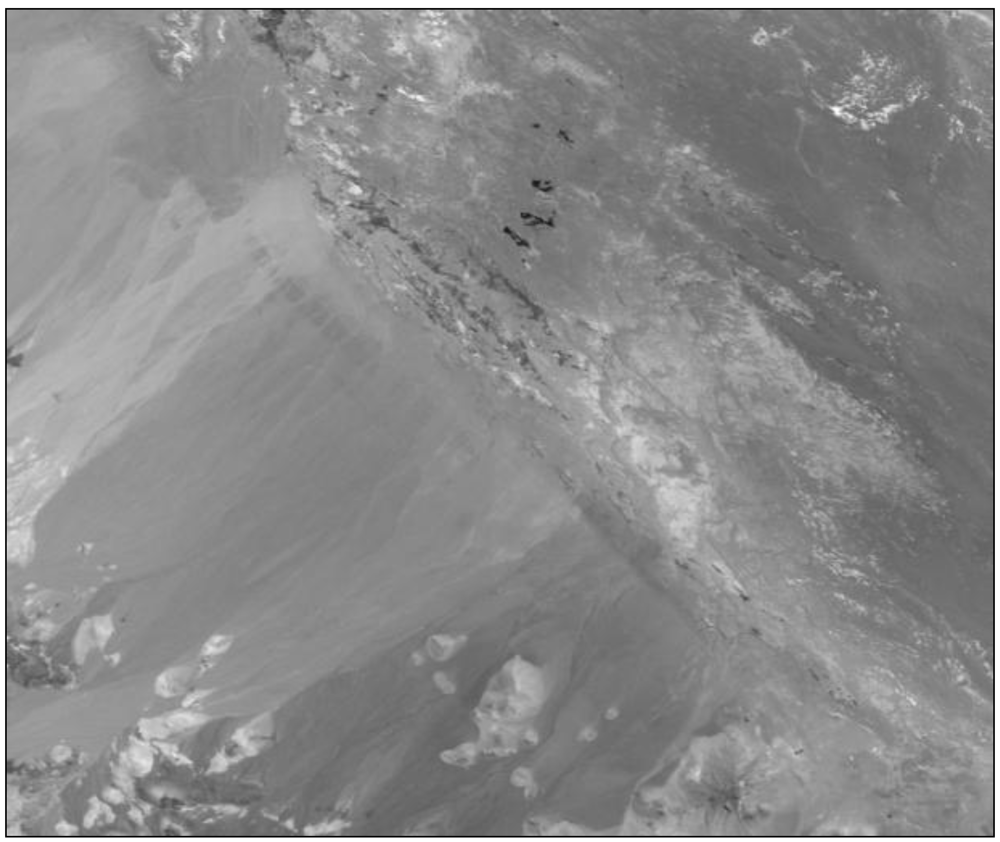
Figure 2 shows the visualization of band 120 of the AVIRIS image Lunar Lake (Scene 01).
Figure 2.
Lunar Lake Scene 01, Band 120.
Figure 2.
Lunar Lake Scene 01, Band 120.
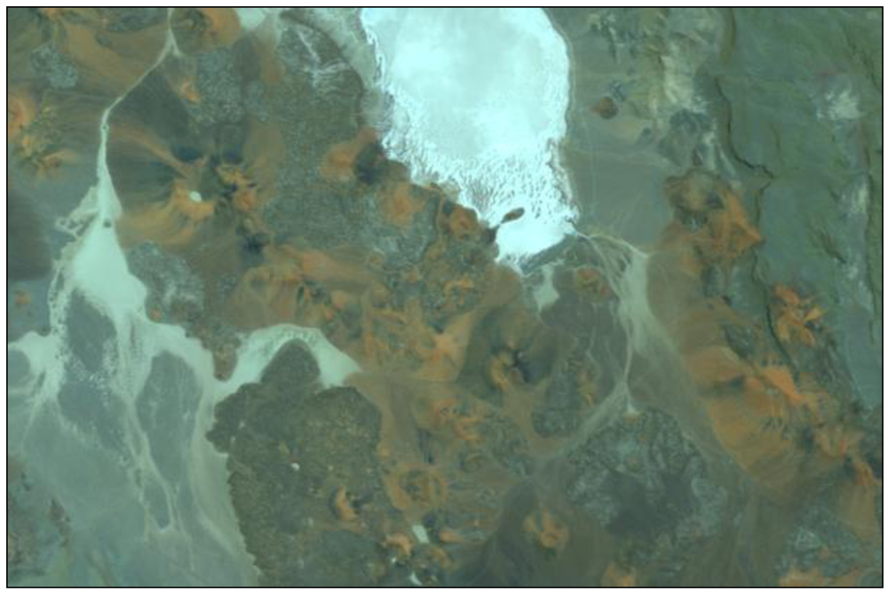
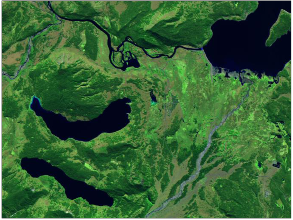
Figure 3 and
Figure 4 show respectively a false colors visualization of the AVIRIS images Lunar Lake Scene 03 and Yellowstone Calibrated Scene 11. The resulting images are generated by assigning band 125 to the red, band 70 to the green and band 30 to the blue.
The accuracy of the hyperspectral sensors is typically measured in spectral resolution, which indicates the bandwidth of the spectrum that is captured. If the scanner picks up a large number of “images” with relatively small bandwidth, then it is possible to identify a large number of objects even if they are located in a relatively small area of pixels.
The JPL (Jet Propulsion Laboratory–NASA) AVIRIS sensor has a spatial resolution that covers an area of 20 × 20 meters per pixel.
The spectral components are obtained via a 12 bits ADC (Analog-to-Digital Converter). The elements of the spectrum, after the necessary calibration and geometric correction, are represented with a16-bit accuracy.
Figure 3.
Lunar Lake Scene 03, with band 125 assigned to the red RGB component, band 70 to the green and band 30 to the blue.
Figure 3.
Lunar Lake Scene 03, with band 125 assigned to the red RGB component, band 70 to the green and band 30 to the blue.
Figure 4.
Yellowstone Scene 11, with band 125 assigned to red component, band 70 to green and band 30 to blue.
Figure 4.
Yellowstone Scene 11, with band 125 assigned to red component, band 70 to green and band 30 to blue.
2.1. Visualization on Google Android OS
In the last few years, mobile devices, such as tablets, smartphones, etc. have increased their potentiality in terms of display resolution, processor capacity and speed. Often, built-in operating systems are specifically designed for these devices (for example Android, iOS, Symbian, etc.) and implement many advanced features. Other features are implemented by third-party applications (also called Apps) that can be installed. The potentiality of these devices prompted us to study this important segment.
Therefore, we have realized a novel implementation of a tool for the visualization of hyperspectral images, similar to the one discussed above. This tool runs on Google Android OS (1.5 or later) ([
14,
15]). The tool reads the image on internal memory or on external data storage (if available), such as SD card, USB pen drive,
etc.
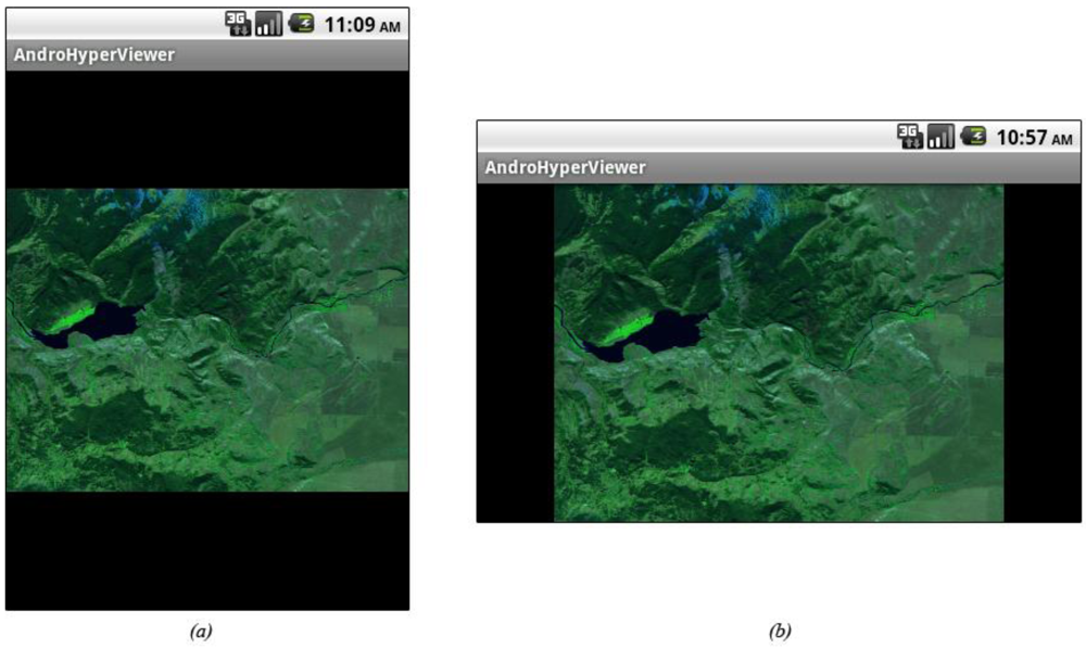
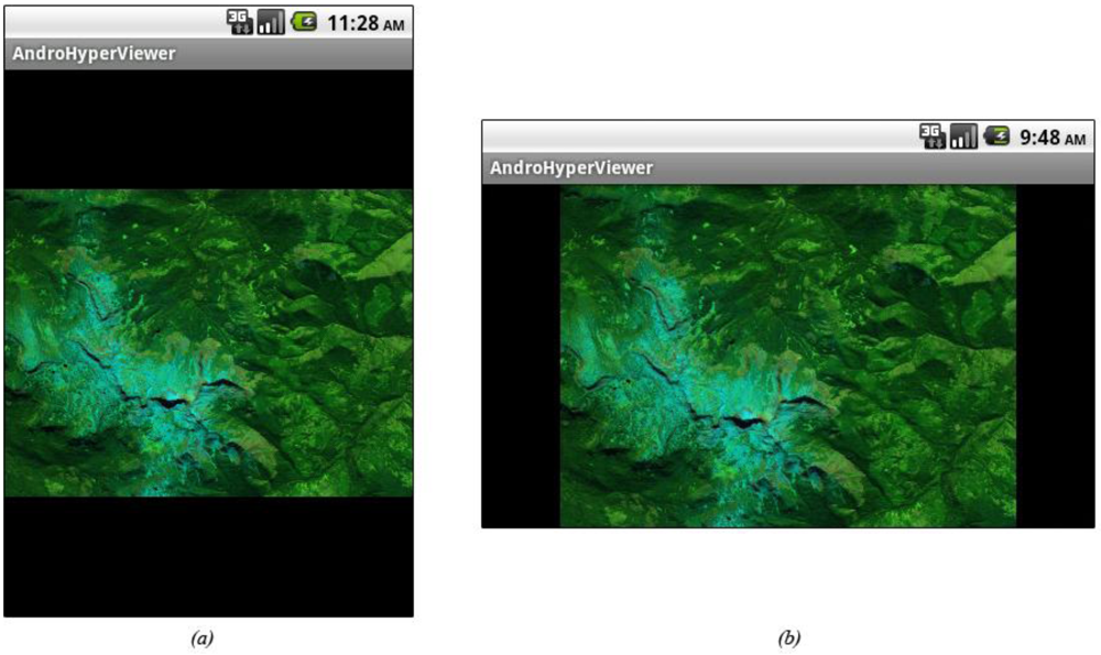
Figure 5 and
Figure 6 show respectively the AVIRIS Yellowstone Calibrated Scene 01 and Scene 18 produced by our tool on the SDK emulator ([
16]) with screen resolution HVGA (480 × 320) in portrait mode (
Figure 5a and
Figure 6a) and in landscape mode (
Figure 5b and
Figure 6b).
Figure 5.
Yellowstone Calibrated Scene 01 on Google Android SDK Emulator in portrait mode and landscape mode with a HVGA screen resolution.
Figure 5.
Yellowstone Calibrated Scene 01 on Google Android SDK Emulator in portrait mode and landscape mode with a HVGA screen resolution.
Figure 6.
Yellowstone Calibrated Scene 18 on Google Android SDK Emulator in portrait mode and landscape mode with a HVGA screen resolution.
Figure 6.
Yellowstone Calibrated Scene 18 on Google Android SDK Emulator in portrait mode and landscape mode with a HVGA screen resolution.
This tool might be helpful in many kinds of applications, as for example the visualization of a hyperspectral image directly on the field.
Moreover, the portability of smartphone devices is certainly important in real application (for example in mineralogy, physics, etc.).
The built-in OS allows some features on touchscreen-based portable devices, such as gestures, pinch-to-zoom, etc., that enable the end user to facilitate use of the tool, without the use of external input peripherals (mouse, keyboards, etc.).
3. Compression of Hyperspectral Data
Compression algorithms that provide lossless or near-lossless quality are generally required to preserve the hyperspectral imagery often acquired at high costs and used in delicate tasks (for instance classification or target detection).
Low complexity compression algorithms may allow on-board implementation with limited hardware capacities, therefore it is often desirable to use this typology of algorithms, for example when the compression process has to be carried out in an airplane or on board a satellite, before transmitting data to the base.
Hyperspectral data presents two forms of correlation:
Spectral correlation is much stronger than spatial correlation. For this reason standard image compression techniques, as for instance the spatial predictor of LOCO-I used in JPEG-LS [
17], fail on this kind of data.
Spectral-oriented Least Squares (SLSQ) [
1,
2,
3,
4,
5,
6,
7] is a lossless hyperspectral image compressor that uses least squares to optimize the predictor for each pixel and each band. As far as we know, SLSQ is the current state-of-the-art in lossless hyperspectral image compression.
Others approaches are, for example, EMPORDA [
18] and a low-complexity and high-efficiency lossy-to-lossless coding scheme proposed in [
19].
The SLSQ approach is based on an optimized linear predictor. SLSQ determines for each sample the coefficients of a linear predictor that is optimal with respect to a three dimensional subset of the past data.
The intra-band distance is defined as:
The inter-band distance is defined as:
The enumerations obtained by using these distances allow the indexing of the pixels from the current pixel.
Similar to the Euclidean distance, the intra-band distance defines the distance of the current pixel with respect to other pixels in the current bands.
The inter-band distance defines the distance of the current pixel with respect to other pixels in the current band and in the previous one. When i = j the d3D distance is the same of the d2D distance.
The pixels that have the same distance are considered in clockwise order for both types of distance.
Figure 7a shows the resulting context for intra-band enumeration;
Figure 7b shows the resulting context for inter-band enumeration.
Figure 7.
The resulting context for intra-band and inter-band enumerations.
Figure 7.
The resulting context for intra-band and inter-band enumerations.
As we can see from
Figure 7b, the indices of the pixels of the (
k − 1)-th band are larger than the indices of these pixels of the
k-th band. This happens because in definition (2) of the inter-band distance the term ¼ is present.
In the following, x(i) denotes the i-th pixel of the intra-band context of the current pixel. x(i,j) denotes the j-th pixel in the inter-band context of x(i).
The N-th order prediction of the current pixel (denoted by x(0, 0)) is computed as:
The coefficients α0 = [α1, …, αN]t minimize the energy of the prediction error, defined as:
We can write P, using matrix notation, as:
where,
The optimal predictor coefficients are the solution of the linear system, defined as:
which is obtained by taking the derivative with respect to α of P, and setting it to zero.
The prediction error, defined as
![Algorithms 05 00076 i015]()
, is entropy coded with an arithmetic coder. A similar prediction structure may be found in [
20].
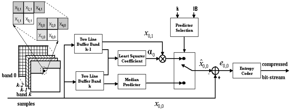
Figure 8.
Spectral oriented Least SQuares (SLSQ) block diagram (from [
1]).
Figure 8.
Spectral oriented Least SQuares (SLSQ) block diagram (from [
1]).
A selector of predictors (as is possible to see in SLSQ block diagram in
Figure 8) is used in [
1]. The role of the selector is to determine which predictor will be used for the prediction of the current pixel.
A standard median predictor is selected if the band of the current sample is in the Intra-Band (IB) set. Otherwise, the SLSQ predictor described above is selected.
4. Efficient Band Ordering
Each band in a hyperspectral image can be seen as a two-dimensional image. By visualizing the content of each band it becomes clear that the spectral correlation is high between many bands, but it is also clear that a few consecutive bands are not strongly spectrally correlated.
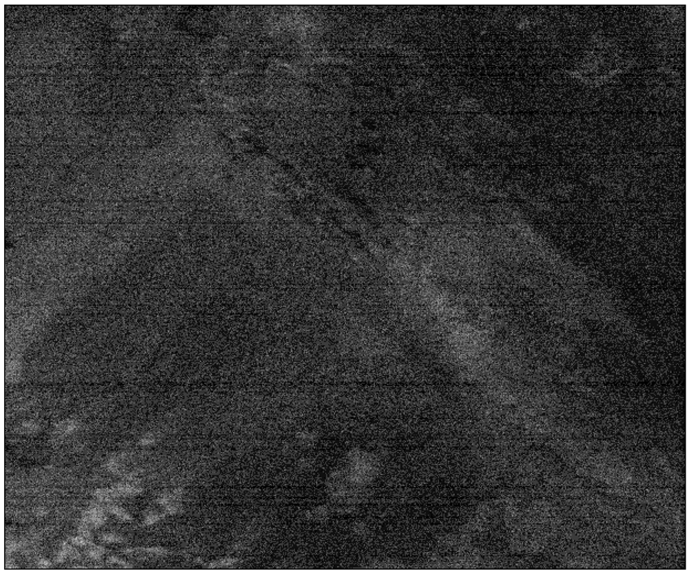
In
Figure 9, for example we show band 160 of the Lunar Lake AVIRIS image.
Figure 9.
Lunar Lake Scene 01, Band 160.
Figure 9.
Lunar Lake Scene 01, Band 160.
If we compare
Figure 9 and
Figure 2 we see that there is very low correlation between the two.
If we are able to analyze the band correlation and if we can re-order the bands, this can lead to improvements to the SLSQ algorithm.
4.1. Band Ordering
The proposed approach can be sub-divided into three step:
The first step consists of making a dependence graph G = (V, E), where each vertex denotes a band and each vertex i is connected, by a weighted edge, with each other vertex j (where i ≠ j).
An edge (i, j)E is weighted as:
w(i, j) = distance between the bandi to the bandj
Now, we are able to compute the Minimum Spanning Tree (MST) on the graph G.
MST allows us to associate each band i (vertex i in the graph G) to its minimum distance band j, therefore to the band where the distance between the band i and the band j is minimal.
The last step consists into computing a Depth First Search (DFS) visit on M. This gives a band ordering, where M is a MST on graph G.
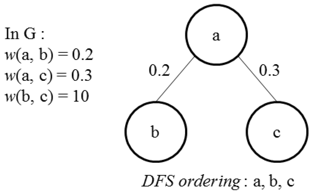
In some cases DFS does not work correctly for our purposes.
In the simple example below we see a case in which DFS does not work correctly for band ordering.
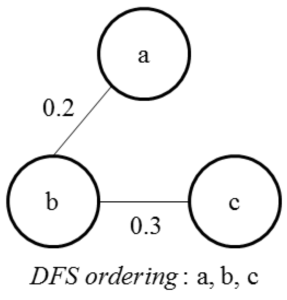
In
Figure 10 the band ordering given by DFS on MST M is
a,
b,
c.
i.e., SLSQ predicts the band
b from the band
a and the band
c from the band
b, but the band
b and the band
c are very low related with respect to band
b and band
a. Therefore it is evident that this band ordering is incorrect.
Figure 10.
Incorrect band ordering given by DFS on MST M.
Figure 10.
Incorrect band ordering given by DFS on MST M.
For these cases we need to modify our approach and introduce band ordering based on DFS and pairs. A pair is defined as:
<previous band in the ordering,current band in the ordering>
In the previous example the band ordering given by a modified DFS visit is therefore <a,b>,<a,c>, this means that SLSQ predicts the band b from the band a and the band c also from the band a, and this is now a correct band ordering.
Figure 11 shows an example in which the DFS visit on the MST M gives a correct band ordering.
Figure 11.
A correct band ordering given by DFS on MST M.
Figure 11.
A correct band ordering given by DFS on MST M.
As we can see in
Figure 11, the band ordering given by the DFS on MST M is correct and the band ordering given by a modified DFS on MST M is
<a,
b>,
<b,
c> that is also correct.
Others approaches of band ordering may be found in [
21].
4.2. Correlation-Based Band Ordering
An important measure of dependence between two random distributions is Pearson’s Correlation [
22]. This measure is obtained by dividing the covariance of two variables by the product of their standard deviation, the formula is defined as:
where σxy is the covariance between X, Y (the two variables).
σx and σy are respectively the standard deviations for X and Y. The Pearson correlation coefficients have values in the range [−1, 1].
When ρxy > 0, the variables are directly correlated. The variables are not correlated when ρxy = 0 and if ρxy < 0, the variables are inversely correlated.
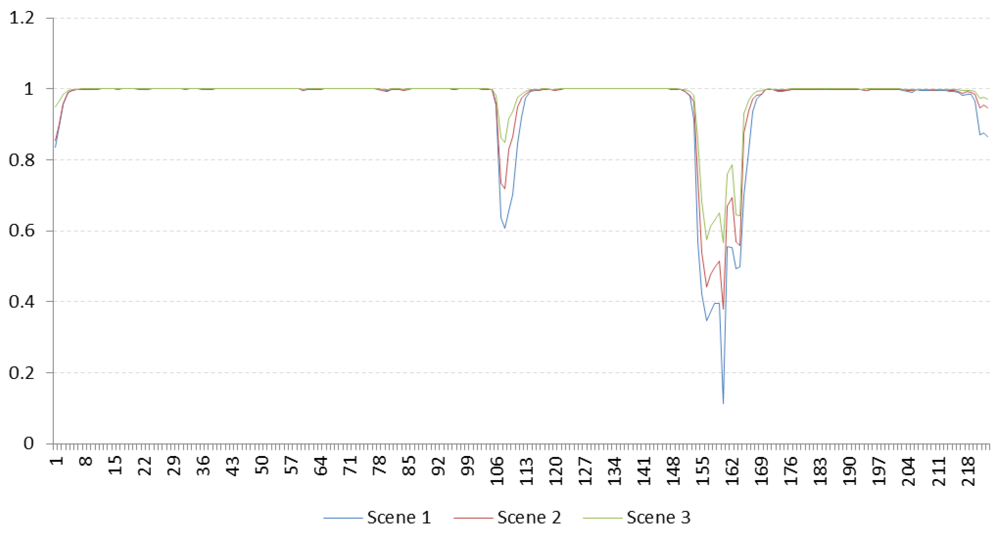
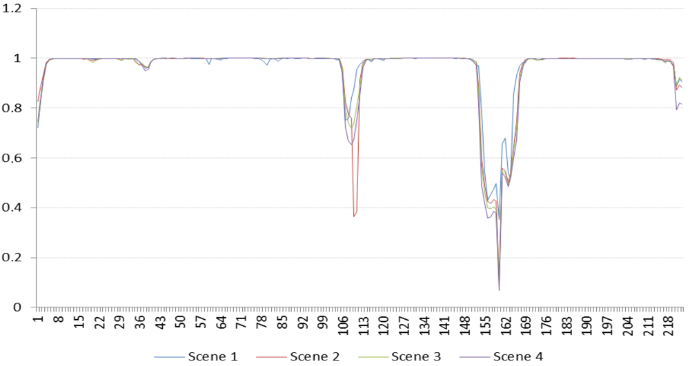
Figure 12,
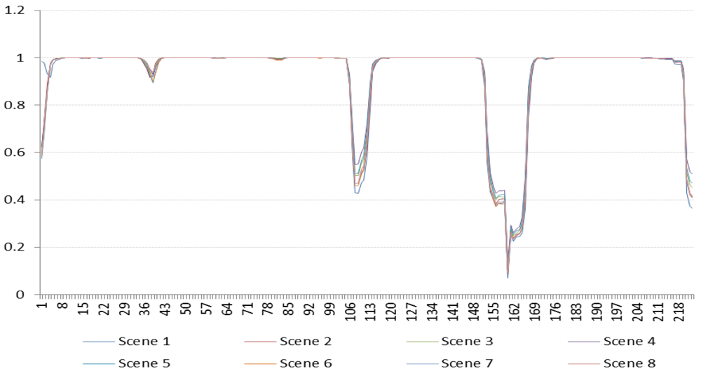
Figure 14,
Figure 16 report the graphs of the Pearson’s correlation for each pair of continuous bands for all the scenes respectively of Lunar Lake, Moffett Field and Low Altitude.
The X axis refers to the x-th pair of bands in the ordering, where the pair is defined as (x-th band, (x + 1)-th band) (for example, without band ordering, the value 1 of the X axis refers to the pair of bands (1, 2), the value 2 refers to the pair of bands (2, 3), and so on) and the Y axis indicates the corresponding value of the Pearson’s correlation between the pair of bands on X axis.
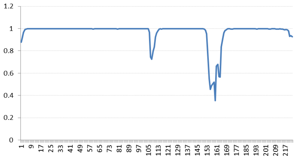
Figure 13 reports the average correlation of all scenes of the Lunar Lake. As in
Figure 13.
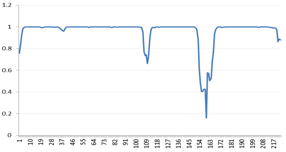
Figure 15 and
Figure 17 report the average correlation of all scenes respectively for Moffett Field and Low Altitude.
Figure 12.
Correlation for continuous band for each scene of Lunar Lake.
Figure 12.
Correlation for continuous band for each scene of Lunar Lake.
Figure 13.
Average scene correlation for continuous band for Lunar Lake.
Figure 13.
Average scene correlation for continuous band for Lunar Lake.
Figure 14.
Correlation for continuous band for each scene of Moffett Field.
Figure 14.
Correlation for continuous band for each scene of Moffett Field.
Figure 15.
Average scene correlation for continuous band for Moffett Field.
Figure 15.
Average scene correlation for continuous band for Moffett Field.
Figure 16.
Correlation for continuous band for each scene of Low Altitude.
Figure 16.
Correlation for continuous band for each scene of Low Altitude.
Figure 17.
Average scene correlation for continuous band for Low Altitude.
Figure 17.
Average scene correlation for continuous band for Low Altitude.
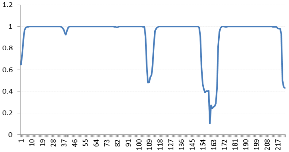
By looking at the above figures we can see that there are many points where there is a discontinuity between continuous bands.
For example, consider the minimum peak in the graph of
Figure 17, regarding the pair of bands (160, 161) (values 160 on the X-axis). The correlation of the pair of bands (160, 161) is approximately 0.102007273, this means that there is very low correlation between those two bands, and this means that the inter-band predictor shall fail its predictions, because there is not enough inter-band correlation.
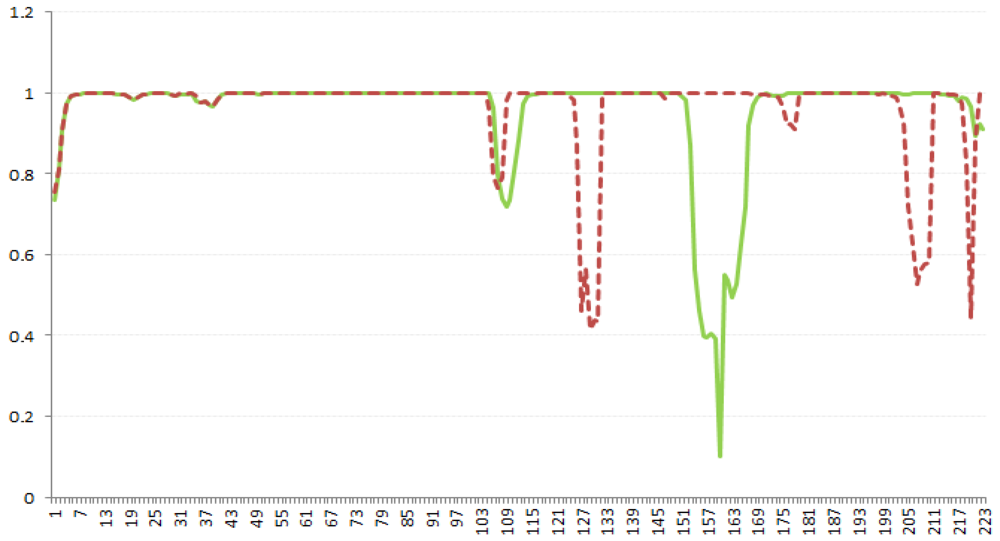
Figure 18 reports the graph of the correlation for continuous band (represented by the green line) and the correlation after the execution of the proposed band ordering (the red dotted line in the graph) for the Scene 03 of Moffett Field.
Figure 18.
The graph reports the trend of the correlation for continuous band (in green) and the trend of the correlation after the execution of the proposed band ordering (in red).
Figure 18.
The graph reports the trend of the correlation for continuous band (in green) and the trend of the correlation after the execution of the proposed band ordering (in red).
From the figure it can be seen that there are less points of discontinuity after the execution of band ordering.
Without band ordering, Pearson’s correlation assumes the minimal value of approximately 0.101975512 (very low correlation).
After band ordering, Pearson’s correlation assumes the value of approximately of 0.415955776 (that means that the bands are correlated).
4.3. Bhattacharyya Distance-Based Band Ordering
We have also considered the Bhattacharyya distance [
23]. For two random distributions, it is defined by probability functions
p1(
x),
p2(
x) as:
When both the distributions are univariate and are assumed to follow normal distribution, the Bhattacharyya distance is defined as:
where μ1, μ2are the means and σ1, σ2 the standard deviations of the two distributions respectively. The result can take values from zero (inclusive) to infinity.
5. Experimental Results
We have tested our Java-based implementation of the SLSQ algorithm on the test data set (a) without band ordering; (b) with Pearson’s correlation-based band ordering; and (c) Bhattacharyya distance-based band ordering.
Our test data set is composed by five NASA AVIRIS hyperspectral images (each one subdivided into scenes): Lunar Lake (3 scenes), Moffett Field (4 scenes), Jasper Ridge (6 scenes), Cuprite (5 scenes) and Low Altitude (8 scenes).
Each scene has 614 columns and 224 spectral bands.
Table 1 reports the compression ratio (C.R.) achieved by SLSQ on the test data set.
Table 1.
Results (C.R. achieved for each scene of the hyperspectral imagery without band ordering).
Table 1.
Results (C.R. achieved for each scene of the hyperspectral imagery without band ordering).
| Lunar Lake | Moffett Field | Jasper Ridge | Cuprite | Low Altitude |
|---|
| Scene | C.R. | Scene | C.R. | Scene | C.R. | Scene | C.R. | Scene | C.R. |
|---|
| Scene 1 | 3.17 | Scene 1 | 3.14 | Scene 1 | 3.20 | Scene 1 | 3.22 | Scene 1 | 3.00 |
| Scene 2 | 3.20 | Scene 2 | 3.18 | Scene 2 | 3.21 | Scene 2 | 3.18 | Scene 2 | 2.98 |
| Scene 3 | 3.21 | Scene 3 | 3.26 | Scene 3 | 3.18 | Scene 3 | 3.21 | Scene 3 | 3.03 |
| | | Scene 4 | 3.11 | Scene 4 | 3.17 | Scene 4 | 3.18 | Scene 4 | 3.01 |
| | | | | Scene 5 | 3.22 | Scene 5 | 3.18 | Scene 5 | 2.99 |
| | | | | Scene 6 | 3.19 | | | Scene 6 | 3.03 |
| | | | | | | | | Scene 7 | 3.03 |
| | | | | | | | | Scene 8 | 3.02 |
The columns indicate respectively the results achieved for Lunar Lake, Moffett Field, Jasper Ridge, Cupirte and Low Altitude.
The IB set used is IB = {1, 2, …, 8}, with M = 4 and N = 1.
Table 2 reports the results achieved in terms of C.R. by SLSQ (with the same settings) by using the proposed band ordering based on Pearson’s Correlation distance. As in
Table 2, the columns indicate respectively the results for scene achieved for Lunar Lake, Moffett Field, Jasper Ridge, Cuprite and Low Altitude.
Table 2.
Results (C.R. achieved for each scene of the hyperspectral imagery with Pearson’s correlation-based band ordering).
Table 2.
Results (C.R. achieved for each scene of the hyperspectral imagery with Pearson’s correlation-based band ordering).
| Lunar Lake | Moffett Field | Jasper Ridge | Cuprite | Low Altitude |
|---|
| Scene | C.R. | Scene | C.R. | Scene | C.R. | Scene | C.R. | Scene | C.R. |
|---|
| Scene 1 | 3.22 | Scene 1 | 3.16 | Scene 1 | 3.23 | Scene 1 | 3.28 | Scene 1 | 3.03 |
| Scene 2 | 3.25 | Scene 2 | 3.20 | Scene 2 | 3.24 | Scene 2 | 3.22 | Scene 2 | 3.01 |
| Scene 3 | 3.26 | Scene 3 | 3.28 | Scene 3 | 3.21 | Scene 3 | 3.26 | Scene 3 | 3.07 |
| | | Scene 4 | 3.14 | Scene 4 | 3.20 | Scene 4 | 3.23 | Scene 4 | 3.05 |
| | | | | Scene 5 | 3.23 | Scene 5 | 3.23 | Scene 5 | 3.02 |
| | | | | Scene 6 | 3.22 | | | Scene 6 | 3.06 |
| | | | | | | | | Scene 7 | 3.06 |
| | | | | | | | | Scene 8 | 3.05 |
Table 3 reports the C.R. achieved by SLSQ by using the same parameters used above, this time for a band ordering based on Bhattacharyya distance.
Table 3.
Results (C.R. achieved for each scene of the hyperspectral imagery with Bhattacharyya distance-based band ordering).
Table 3.
Results (C.R. achieved for each scene of the hyperspectral imagery with Bhattacharyya distance-based band ordering).
| Lunar Lake | Moffett Field | Jasper Ridge | Cuprite | Low Altitude |
|---|
| Scene | C.R. | Scene | C.R. | Scene | C.R. | Scene | C.R. | Scene | C.R. |
|---|
| Scene 1 | 2.96 | Scene 1 | 2.71 | Scene 1 | 2.88 | Scene 1 | 3.07 | Scene 1 | 2.75 |
| Scene 2 | 3.02 | Scene 2 | 2.78 | Scene 2 | 2.86 | Scene 2 | 2.93 | Scene 2 | 2.72 |
| Scene 3 | 3.06 | Scene 3 | 2.94 | Scene 3 | 2.83 | Scene 3 | 3.00 | Scene 3 | 2.81 |
| | | Scene 4 | 2.65 | Scene 4 | 2.78 | Scene 4 | 3.01 | Scene 4 | 2.80 |
| | | | | Scene 5 | 2.89 | Scene 5 | 3.03 | Scene 5 | 2.76 |
| | | | | Scene 6 | 2.87 | | | Scene 6 | 2.81 |
| | | | | | | | | Scene 7 | 2.81 |
| | | | | | | | | Scene 8 | 2.78 |
The following tables (
Table 4,
Table 5 and
Table 6) report the achieved results in terms of Bit-Per-Pixel (BPP).
Table 4 reports achieved results scene-by-scene for each hyperspectral image without band ordering,
Table 5 similarly
Table 2 reports achieved results in terms of BPP with proposed band ordering based on Pearson’s correlation distance.
Table 6 reports the achieved results in terms of BPP by SLSQ with Bhattacharyya distance-based band ordering.
Table 4.
Results (BPP achieved for each scene of the hyperspectral imagery without band ordering).
Table 4.
Results (BPP achieved for each scene of the hyperspectral imagery without band ordering).
| Lunar Lake | Moffett Field | Jasper Ridge | Cuprite | Low Altitude |
|---|
| Scene | BPP | Scene | BPP | Scene | BPP | Scene | BPP | Scene | BPP |
|---|
| Scene 1 | 5.05 | Scene 1 | 5.09 | Scene 1 | 5.00 | Scene 1 | 4.96 | Scene 1 | 5.34 |
| Scene 2 | 5.00 | Scene 2 | 5.03 | Scene 2 | 4.99 | Scene 2 | 5.03 | Scene 2 | 5.36 |
| Scene 3 | 4.98 | Scene 3 | 4.91 | Scene 3 | 5.04 | Scene 3 | 4.98 | Scene 3 | 5.27 |
| | | Scene 4 | 5.14 | Scene 4 | 5.04 | Scene 4 | 5.02 | Scene 4 | 5.31 |
| | | | | Scene 5 | 4.99 | Scene 5 | 5.03 | Scene 5 | 5.35 |
| | | | | Scene 6 | 5.02 | | | Scene 6 | 5.28 |
| | | | | | | | | Scene 7 | 5.28 |
| | | | | | | | | Scene 8 | 5.30 |
Table 5.
Results (BPP achieved for each scene of the hyperspectral imagery with Pearson’s correlation-based band ordering).
Table 5.
Results (BPP achieved for each scene of the hyperspectral imagery with Pearson’s correlation-based band ordering).
| Lunar Lake | Moffett Field | Jasper Ridge | Cuprite | Low Altitude |
|---|
| Scene | BPP | Scene | BPP | Scene | BPP | Scene | BPP | Scene | BPP |
|---|
| Scene 1 | 4.98 | Scene 1 | 5.06 | Scene 1 | 4.95 | Scene 1 | 4.88 | Scene 1 | 5.28 |
| Scene 2 | 4.92 | Scene 2 | 5.00 | Scene 2 | 4.94 | Scene 2 | 4.96 | Scene 2 | 5.31 |
| Scene 3 | 4.90 | Scene 3 | 4.88 | Scene 3 | 4.99 | Scene 3 | 4.91 | Scene 3 | 5.22 |
| | | Scene 4 | 5.09 | Scene 4 | 4.99 | Scene 4 | 4.96 | Scene 4 | 5.25 |
| | | | | Scene 5 | 4.95 | Scene 5 | 4.95 | Scene 5 | 5.30 |
| | | | | Scene 6 | 4.97 | | | Scene 6 | 5.23 |
| | | | | | | | | Scene 7 | 5.22 |
| | | | | | | | | Scene 8 | 5.24 |
Table 6.
Results (BPP achieved for each scene of the hyperspectral imagery with Bhattacharyya distance-based band ordering).
Table 6.
Results (BPP achieved for each scene of the hyperspectral imagery with Bhattacharyya distance-based band ordering).
| Lunar Lake | Moffett Field | Jasper Ridge | Cuprite | Low Altitude |
|---|
| Scene | BPP | Scene | BPP | Scene | BPP | Scene | BPP | Scene | BPP |
|---|
| Scene 1 | 5.40 | Scene 1 | 5.89 | Scene 1 | 5.56 | Scene 1 | 5.20 | Scene 1 | 5.83 |
| Scene 2 | 5.30 | Scene 2 | 5.76 | Scene 2 | 5.59 | Scene 2 | 5.45 | Scene 2 | 5.87 |
| Scene 3 | 5.24 | Scene 3 | 5.44 | Scene 3 | 5.66 | Scene 3 | 5.34 | Scene 3 | 5.69 |
| | | Scene 4 | 6.04 | Scene 4 | 5.76 | Scene 4 | 5.31 | Scene 4 | 5.72 |
| | | | | Scene 5 | 5.54 | Scene 5 | 5.28 | Scene 5 | 5.80 |
| | | | | Scene 6 | 5.58 | | | Scene 6 | 5.70 |
| | | | | | | | | Scene 7 | 5.71 |
| | | | | | | | | Scene 8 | 5.75 |
The following table (
Table 7) reports average results achieved without band ordering (first column), with Correlation-based band ordering (second column) and Bhattacharyya distance-based band ordering (third column). The last row shows the resulting average for each type of band ordering.
Table 7.
Average results in terms of C.R. for each hyperspectral image without ordering, with Pearson’s correlation-based band ordering and Bhattacharyya distance-based band ordering.
Table 7.
Average results in terms of C.R. for each hyperspectral image without ordering, with Pearson’s correlation-based band ordering and Bhattacharyya distance-based band ordering.
| Without band ordering | Correlation-based band ordering | Bhattacharyya-based band ordering |
|---|
| Lunar Lake | 3.19 | 3.24 | 3.01 |
| Moffett Field | 3.17 | 3.20 | 2.77 |
| Jasper Ridge | 3.19 | 3.22 | 2.85 |
| Cuprite | 3.19 | 3.24 | 3.00 |
| Low Altitude | 3.01 | 3.04 | 2.78 |
| Average | 3.15 | 3.19 | 2.88 |
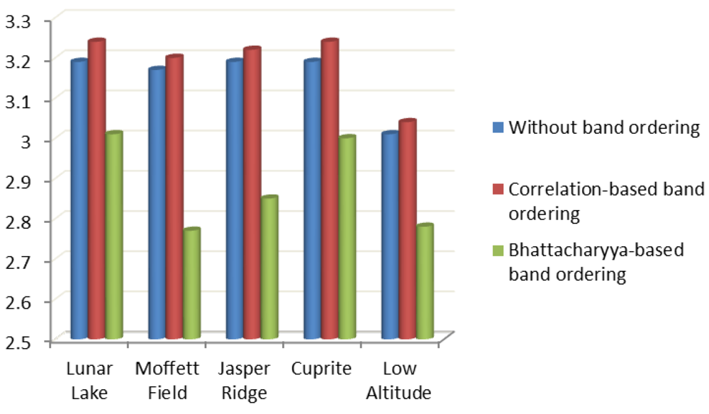
Figure 19 shows the histogram for achieved average results in terms of C.R. Each set of three cones indicates respectively results without band ordering, with Pearson’s Correlation-based band ordering and Bhattacharyya-based band ordering for each image (on the X axis). The Y-axis indicates the C.R. achieved.
Figure 19.
Average results in terms of C.R.–Histogram.
Figure 19.
Average results in terms of C.R.–Histogram.
Results Analysis
From the observation of the experimental results it is clear that band ordering based on Pearson’s Correlation improves the lossless compression of hyperspectral images.
Contrariwise, the results achieved with the band ordering based on Bhattacharyya distance are worst with respect to the results achieved without band ordering.
Therefore, in our experiments Bhattacharyya distance does not work correctly for our purposes.
In detail, the average improvement introduced with the Pearson’s correlation-based band ordering is in terms of 0.04 on C.R. (approximately +1.27%) with respect to the achieved results without band ordering.
Instead, the results achieved with band ordering based on Bhattacharyya distance are worst with respect to the results without band ordering in terms of −0.27 on C.R. (approximately −8.5%).
6. Conclusions and Future Work
Visualization, band ordering and compression of hyperspectral data are topics of interest in the remote sensing field.
For visualization we consider the visualization of single bands of the hyperspectral data or a combined visualization of three bands, where each band is assigned to a separate RGB component.
We have shown how to perform this visualization and have implemented a visualization tool for portable devices.
We then studied the lossless compression of hyperspectral images and examined the Spectral oriented Least SQuares (SLSQ) algorithm.
SLSQ is an efficient and low complexity algorithm for the lossless compression of hyperspectral images, it is suitable for on-board implementation. We have proposed our Java-based implementation of SLSQ.
Finally we have considered band ordering for hyperspectral image compression.
We have proposed an efficient band ordering approach that leads to improvements to SLSQ performance. The proposed approach is based on two metrics: Pearson’s Correlation and Bhattacharyya distance.
The experimental results achieved by our Java-based implementation of the SLSQ algorithm respectively without band ordering, with band ordering based on Pearson’s Correlation and with band ordering based on Bhattacharyya distance have been examined.
The band ordering based on Pearson’s Correlation achieved the best experimental performance.
The results achieved by the band ordering based on Bhattacharyya distance instead are not good enough when compared to the results achieved without band ordering.
In the future we will also test the proposed approach with other distance measures.
Future work will also include improvements for the tool we have developed for the visualization of hyperspectral imagery.


 , is entropy coded with an arithmetic coder. A similar prediction structure may be found in [20].


