1. Introduction
Approximation of set-valued functions has various potential applications in optimization, mathematical economics, control, robotics and more. While approximation of set-valued functions with convex sets as images can be achieved with methods based on
Minkowski averages c.f. [
1], it is shown in [
2] that Minkowski averages are not suitable for approximation of set-valued functions with general (not necessarily convex) images. In order to develop approximation methods for set-valued functions with general images, other averaging operations on compact sets are required. Along with theoretical construction of such averaging operations, efficient algorithms for their computation are needed.
First introduced by Z. Artstein in [
3], the
metric average of two compact sets in
is a union of weighted averages between any point from any of the two sets and the subset of all its closest points from the other set. The interest in the metric average is due to its
metric property in relation to the Hausdorff distance [
3]. The metric property of the metric average is that its Hausdorff distance from any of the averaged sets changes linearly with the weight parameter of the average.
In [
3], the metric average is used for piecewise linear approximation of set-valued functions. Extending these results, Dyn
et al. applied the metric average to the approximation of set-valued functions from a finite number of their samples, using spline subdivision schemes and more generally positive approximation operators [
4,
5]. These methods are based on repeated computations of the metric average.
The applicability of metric average based approximation methods requires efficient algorithms for the computation of the metric average of compact sets. An algorithm for the computation of the metric average of two 1D compact sets with computation time, which is linear in the number of connected subsets in the two sets, is introduced in [
6]. A first step in the development of algorithms for the computation of the metric average of 2D sets is done in [
7], where an algorithm for the computation of the metric average of two intersecting convex polygons is introduced and analyzed. The algorithm of [
7] has linear time complexity in the number of vertices of the input polygons.
In this work we introduce an algorithm that applies tools of computation geometry, segment Voronoi diagrams (
c.f. [
8]) and planar arrangements (
c.f. [
9]) to the computation of the metric average of 2D sets with piecewise linear boundaries. Such sets are collections of simple polygons and of simple polygons with holes. Since a compact 2D set with boundary consisting of closed curves can be linearly approximated by a 2D set with piecewise linear boundaries, our algorithm provides a computational method for approximation of set-valued functions with 2D images from a finite number of samples.
Although the definition of the metric average of two sets with piecewise linear boundaries requires at least one operation for each point in the two sets, our algorithm reduces the computation to boundaries of cells of the partition of the two sets, obtained by the segment Voronoi diagram. The complexity of the algorithm is , where n is the total number of vertices on the boundaries of the two sets.
Our algorithm is based on geometric objects such as segment Voronoi diagrams, arrangements of conic arcs and conic polygons with holes. We implemented the algorithm in C++, using the CGAL library [
10], for handling the various geometric objects.
The outline of this paper is as follows.
Section 2 contains definitions and notation. In particular we review the main geometric concepts relevant to our work such as the metric average, segment Voronoi diagrams, planar arrangements and conic polygons with holes. In
Section 3 we present the algorithm for the computation of the metric average of two simple polygons. The algorithm is extended to general 2D sets with piecewise linear boundaries in
Section 4. Examples of the metric average computed by our algorithm, are presented in
Section 5. In
Section 6 we derive the run-time complexity bounds for our algorithm and obtain bounds on the combinatorial complexity of the computed metric average. Conclusions and directions for possible extensions are given in
Section 7.
2. Preliminaries
To define the metric average of two sets, we first introduce some notation. The
Euclidean distance from a point
p to a set
is
with
the Euclidean norm. A point
q is called a
projection point of a point
p on a set
A, if
q belongs to the
closure of
A and
. Generally the projection point is not unique, and the set of all projection points of
p on
A is denoted by
. For two sets
and
, we introduce the asymmetric operation
, which is the set of all
t-weighted averages between any point in
A and all its projection points on
B, namely
Finally the
t-weighted
metric average of two compact sets
is defined as,
It is easy to verify that
,
, and
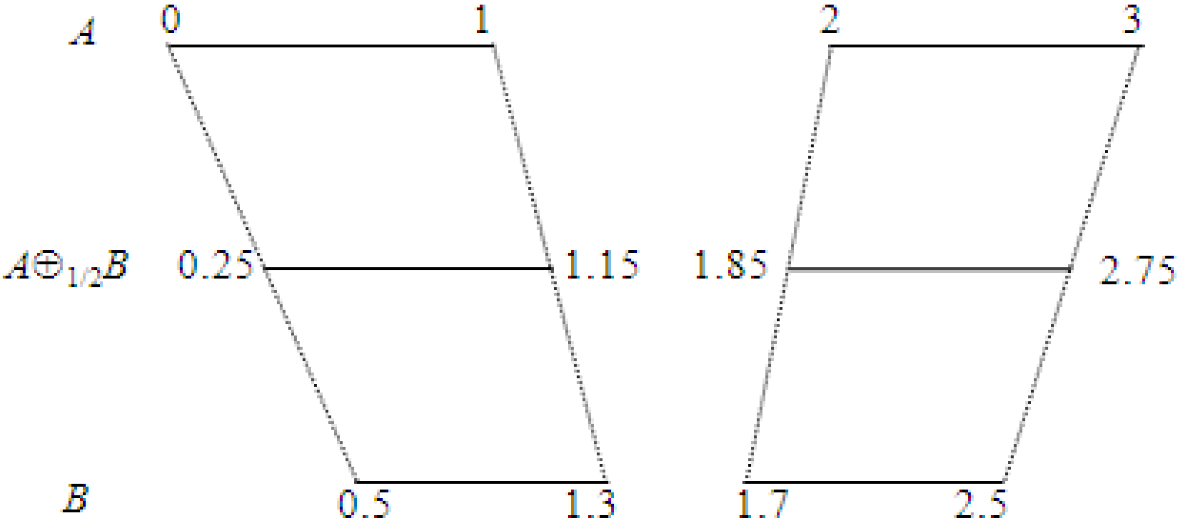
. An example of the metric average of two sets in 1D is given in
Figure 1.
Since for
, the projection point of
p on
A, and also the projection point of
p on
B is the point
p itself, we have
where ∖ denotes the usual set difference.
Now since for points outside a set, the projection on the set is equivalent to the projection on the boundary of the set, relation (2.3) can be further rewritten as,
where
∂ denotes the boundary of a set.
Next we briefly recall the definitions of the geometric objects used in this work. A collection of points
satisfying
with
, is called a
planar conic curve. We refer to segments of conic curves as
conic segments.
A
simple polygon is a region of the plane bounded by a single closed and not self-intersecting chain of linear segments, termed
edges. A
simple polygon with holes is a simple polygon that contains holes,
Figure 1.
The metric average of two non-convex sets in 1D, where , , .
Figure 1.
The metric average of two non-convex sets in 1D, where , , .
which are simple polygons. If we allow the edges to be conic segments, we get a
simple conic polygon with holes. A set with piecewise linear boundaries is a collection of pairwise disjoint simple polygons with holes.
A collection of simple conic polygons with holes can be treated as a
planar arrangement (
c.f. [
9]). Given a set
C of bounded planar curves, the arrangement
is the subdivision of the plane induced by the curves in
C into zero-dimensional, one-dimensional and two-dimensional cells, called
vertices,
edges and
faces respectively. The
overlay of two arrangements
is the arrangement
produced by the edges from
and
.
Given a collection Σ of geometric objects in
, called
Voronoi sites, the
Voronoi diagram (see e.g. [
8,
11]) of Σ is the subdivision of the plane into regions (called
Voronoi faces), each region being associated with a site
, and containing all points of the plane for which
is closest (with respect to the Euclidean distance) among all the sites in Σ. A
Voronoi bisector is a set of points that are equidistant from two Voronoi sites. The Voronoi diagram induced by a collection of linear segments in
is termed
segment Voronoi diagram. The standard technique is to treat a segment as three disjoint geometric objects: two endpoints and an open segment [
8]. The bisector between an open segment
and a point
is defined by the line through
that is perpendicular to
. We also assume that the diagram is bounded by a rectangular frame, which is large enough not to influence the computation of the metric average.
3. The Algorithm for Simple Polygons
Here we assume that are simple polygons. We begin with the representation (2.4) of the metric average. The main part of the computation of the metric average is the computation of the sets and with . We describe in details the computation of . First we apply a sequence of reductions, which simplify the computations. The main idea is to partition by the segment Voronoi diagram induced by . We show that it is sufficient to perform the computations only on the boundary curves of the cells of this partition.
Denote by
the collection of faces of the segment Voronoi diagram induced by the
. The Voronoi faces in
constitute a partition of the plane. Therefore the set
can be represented as,
and thus, by the definition of
in (2.1),
Denoting by
the Voronoi site associated with a Voronoi face
F, we observe that by the definition of
, the closest point on
to
is on
, and obtain
We call a connected component of
with non-empty interior a
metric face of
F. For
a metric face of
F, we define
. We denote by
the collection of all the metric faces induced by the Voronoi faces in
and by
. With this notation (3.3) can be rewritten as,
In order to compute using the reduction (3.4), it is required first to find the metric faces and then for each metric face F to compute ,
The computation of the metric faces are based on planar arrangements. The bisectors of the segment Voronoi diagram are conic curves [
8], hence
constitutes an arrangement of conic segments. Obviously
can be represented by an arrangement of linear segments. Thus the metric faces are the intersections of the bounded faces of the two arrangements and can be computed by the overlay of these two arrangements.
Next we show that the computation of
for a metric face
F can be further reduced to the computation of
. The Voronoi site
is either an open linear segment or a point, thus the set
of all projection points of a point
on
is a singleton. It is easy to see, that the operation
, can be regarded as a continuous one-to-one function from the metric face
F to
. Consequently,
is a simple closed curve, since the boundary of a metric face is so. Thus the region bounded by
is
, and it is sufficient to compute
. Denoting by
the region bounded by
, we have
Finally the computation is reduced to that of for a conic segment τ on the boundary of a metric face F. This straightforward task is completed by a fixed number of operations. The obtained set is also a conic segment, and therefore is a conic polygon.
To conclude, our algorithm computes the metric average of two simple polygons using (2.4), (3.4) and (3.5), and
where
is the collection of conic segments comprising
.
4. Extension to 2D Sets with Piecewise Linear Boundaries
The algorithm for the computation of the metric average of two simple polygons introduced in the previous section can be straightforwardly extended to 2D sets with piecewise linear boundaries, namely each set is a collection of simple polygons with holes. We discuss the computation of with such sets .
The boundary of B consists of linear segments and therefore the segment Voronoi diagram is well defined. The metric faces are defined as in the previous section, and Relations (3.1)-(3.4) stay valid. However a metric face F is now a connected component of the intersection of a Voronoi face with a collection of simple polygons with holes, so it is a simple conic polygon with holes. Let a metric face F be a simple conic polygon P with holes . The arguments of the previous section imply that is a simple conic polygon with holes . Consequently, the computation of is reduced to the computation of and .
5. Examples
We implemented the algorithm in C++, using the CGAL library [
10] for computational geometry algorithms. In particular we used [
12] for 2D arrangements, [
13] for segment Voronoi diagrams and [
14] for Boolean set operations. The input to the algorithm is two collections of polygons with holes comprising the input sets, and the output is a collection of conic polygons with holes comprising the computed metric average.
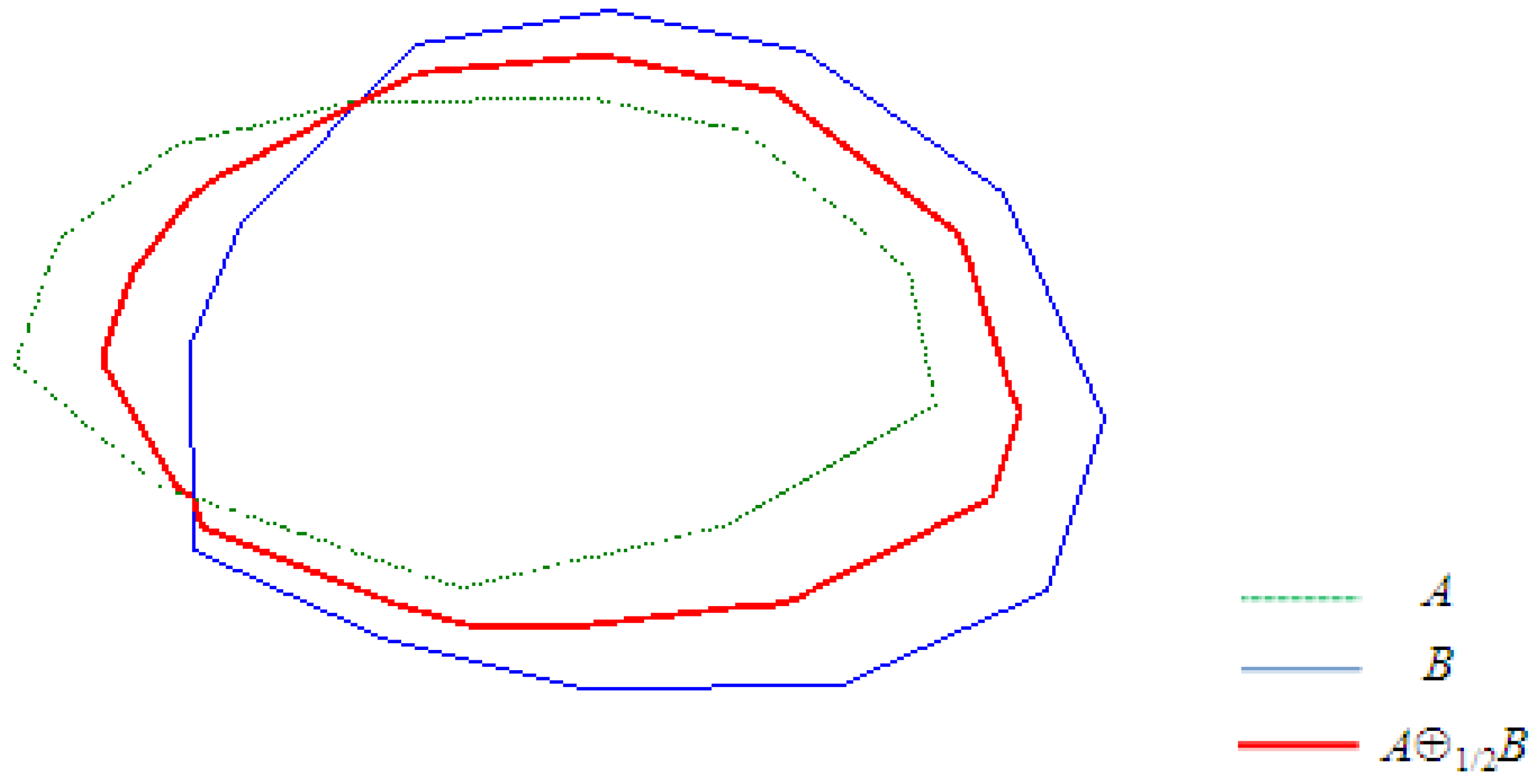
We present a collection of examples of the metric average of two sets with piecewise linear boundaries. In the following examples the boundaries of the input sets are depicted in dotted green and blue respectively, and the boundary of their metric average is depicted in bold red.
Figure 2.
where are simple convex polygons.
Figure 2.
where are simple convex polygons.
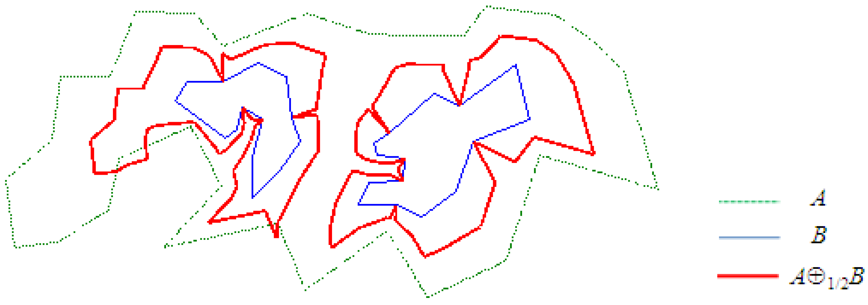
Figure 3.
, where A is a simple polygon and B consists of two simple polygons included in A.
Figure 3.
, where A is a simple polygon and B consists of two simple polygons included in A.
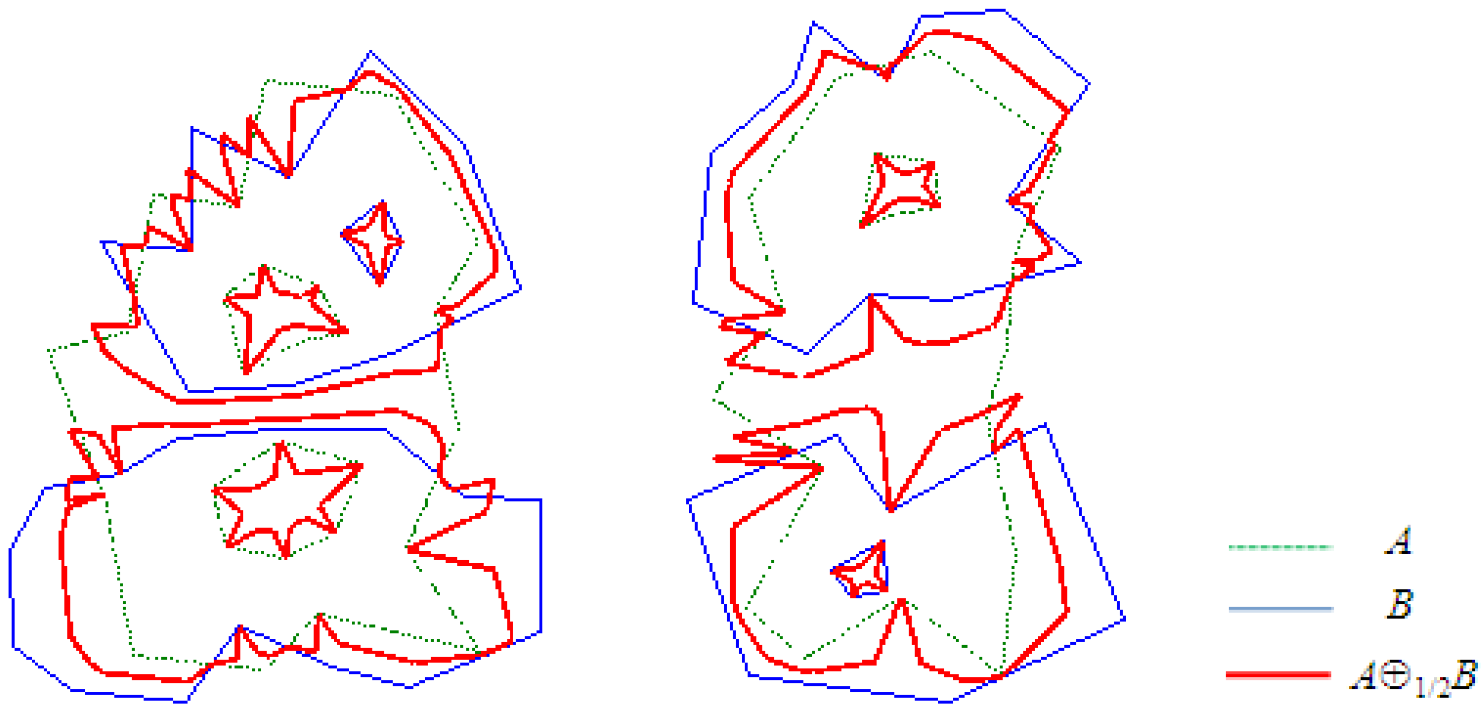
Figure 4.
, where are sets with piecewise linear boundaries.
Figure 4.
, where are sets with piecewise linear boundaries.
The examples indicate that the metric average is more suitable for applications of set-valued approximation, where the Hausdorff distance between the sampled function and the approximant is of interest, but it is less suitable for geometry oriented applications. The geometric “artifacts” produced by the metric average are explained by the fact that the projection point on a set may move discontinuously for points near the boundaries between faces of the Voronoi diagram induced by the boundary of the set.
6. Complexity Bounds
In this section we discuss the run-time complexity bounds for our algorithm and the combinatorial complexity of the obtained set. We assume here that are simple polygons, and the extension of the results of this section to 2D sets with piecewise linear boundaries is straightforward. The complexity bounds depend on the well known complexity of the underlying algorithms for the computation of segment Voronoi diagrams and planar arrangements.
Recall that by (2.4) and (3.4),
Our main task in this complexity analysis is to show that (6.1) is a union of simple conic polygons with pairwise disjoint interiors. For this goal, we first prove several results about the metric average that will be later used in the complexity analysis.
Lemma 6.1 Let
such that
, then for
Proof. Assume to the contrary that there exists a point
p in
, then there exist
such that
From above equality we conclude that
. Without loss of generality assume, that
Recall, by definition, that
Since
and
, (6.2) implies
. Thus by (6.3),
in contradiction to (6.4).
☐
An immediate consequence of Lemma 6.1 is
Corollary 6.2 Let , then there is a unique point , denoted by , such that . Moreover simple geometric arguments imply that for , .
Since any two metric faces contained in the same polygon have disjoint interiors, we conclude from the above lemma,
Corollary 6.3 Let be metric faces such that , then and have disjoint interiors.
Next we prove a result complementing Lemma 6.1.
Lemma 6.4 Let
,
. If
then
Proof. Let
, then there exist points
and
such that
Without loss of generality assume that
By definition,
By (6.5) and (6.6),
We prove the lemma by contradiction. Suppose
, then by (6.5)
. Thus
, and therefore by (6.8)
, which is a contradiction to (6.7).
☐
Note that under the conditions of Lemma 6.4, and , and therefore we get, in view of Corollary 6.2, that
Corollary 6.5 The sets have pairwise disjoint interiors.
Next we discuss the combinatorial complexity of the metric average of two simple polygons. The discussion is based on the notion of the combinatorial complexity of a planar arrangement, which is the sum of the number of vertices, the number of edges, and the number of faces in the arrangement.
Proposition 6.6 Let n be the sum of the numbers of vertices in A and in B. The combinatorial complexity of with is .
Proof. The combinatorial complexity of
is
and the combinatorial complexity of
is
[
8]. Since the metric faces in
are partial to the overlay of the arrangements representing
and
their total combinatorial complexity is
and the same bound holds for the metric faces in
. By Corollaries 6.3 and 6.5, (6.1) is a union of sets with pairwise disjoint interiors. So the combinatorial complexity of
is bounded by the combinatorial complexity of
and the combinatorial complexity of the metric faces, namely it is
.
☐
Finally we derive the run-time complexity of our algorithm.
Proposition 6.7 Let n be the sum of the numbers of vertices in A and in B. Let k be the combinatorial complexity of the overlay of the arrangements representing and . Then the run-time complexity of the computation of the metric average is .
Proof. It follows from the proof of Proposition 6.6 that
k is
. Computation of the sets
,
,
can be done in
and the combinatorial complexity of each of these sets is bounded by
k [
15]. The segment Voronoi diagrams
and
can be computed in
[
8]. Since the metric faces in
are computed by the overlay of the arrangements representing
and
, with the combinatorial complexity of the result bounded by
k, they can be found in
. Computation of
for all metric faces in
is performed in
. The same bounds hold for metric faces in
. Finally we compute
as in (6.1). By the proof of Proposition 6.6 the combinatorial complexity of
is
, so the corresponding arrangement can be computed in
[
9,
15].
☐
7. Conclusions
In this work we present an algorithm for the computation of the metric average of 2D sets with piecewise linear boundaries. Our algorithm provides a computational method for the approximation of set valued functions with images in
from a finite number of samples, by techniques based on the metric average [
3,
4,
5].
Although the metric average of 2D sets is defined by operations on each point in the two operand sets, our algorithm reduces the computation to manipulation of 1D objects. This is achieved using segment Voronoi diagrams and planar arrangements. The implementation of the algorithm uses the relevant geometric algorithms in the CGAL [
10] library.
The main idea of our algorithm, namely the simplification of the computation of the metric average with Voronoi diagrams has straightforward extension to any two objects in any finite dimension, such that the Voronoi diagrams of the boundaries of the two objects are well defined. A natural extension of this work is to develop and implement an algorithm for the computation of the metric average of two polyhedra.
Whereas the metric average is of interest in applications where the Hausdorff distance is important, it does not possess good geometric properties, as is indicated by the examples in
Section 5. For geometric applications, it is of interest to develop set averaging operations that possess good geometric properties, i.e. comprise a gradual transformation of the geometric shape between the two sets, and also have the “metric property” relative to some metric. The first two authors have recently developed a new set averaging operation with good geometric features, having the “metric property” relative to the measure of the symmetric difference of two sets [
16].
