A Bayesian Algorithm for Functional Mapping of Dynamic Complex Traits

Abstract
:1. Introduction
2. Bayesian Functional Mapping
2.1. Linear Model
2.2. Modeling the Mean-Covariance Structures
2.3. Likelihood
2.4. Parameter Estimation and Algorithm
Estimation theory
Algorithm implementation
Estimation issues
2.5. Structuring the Covariance Matrix
Autoregressive model
Structured Antedependence Model
2.6. Bayes Factor
3. A Worked Example
3.1. Mapping Population
3.2. Results

| Parameter | ||||||
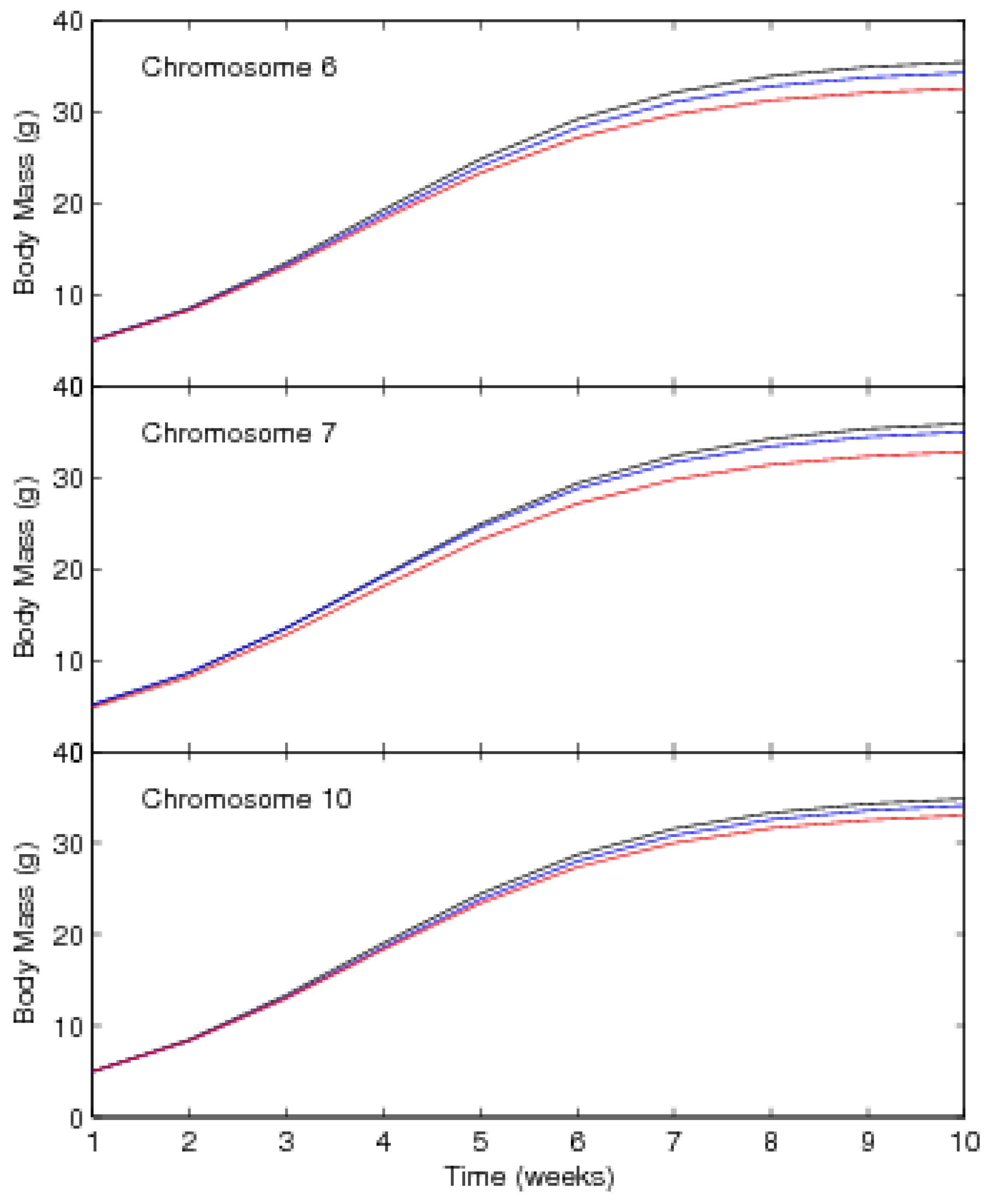
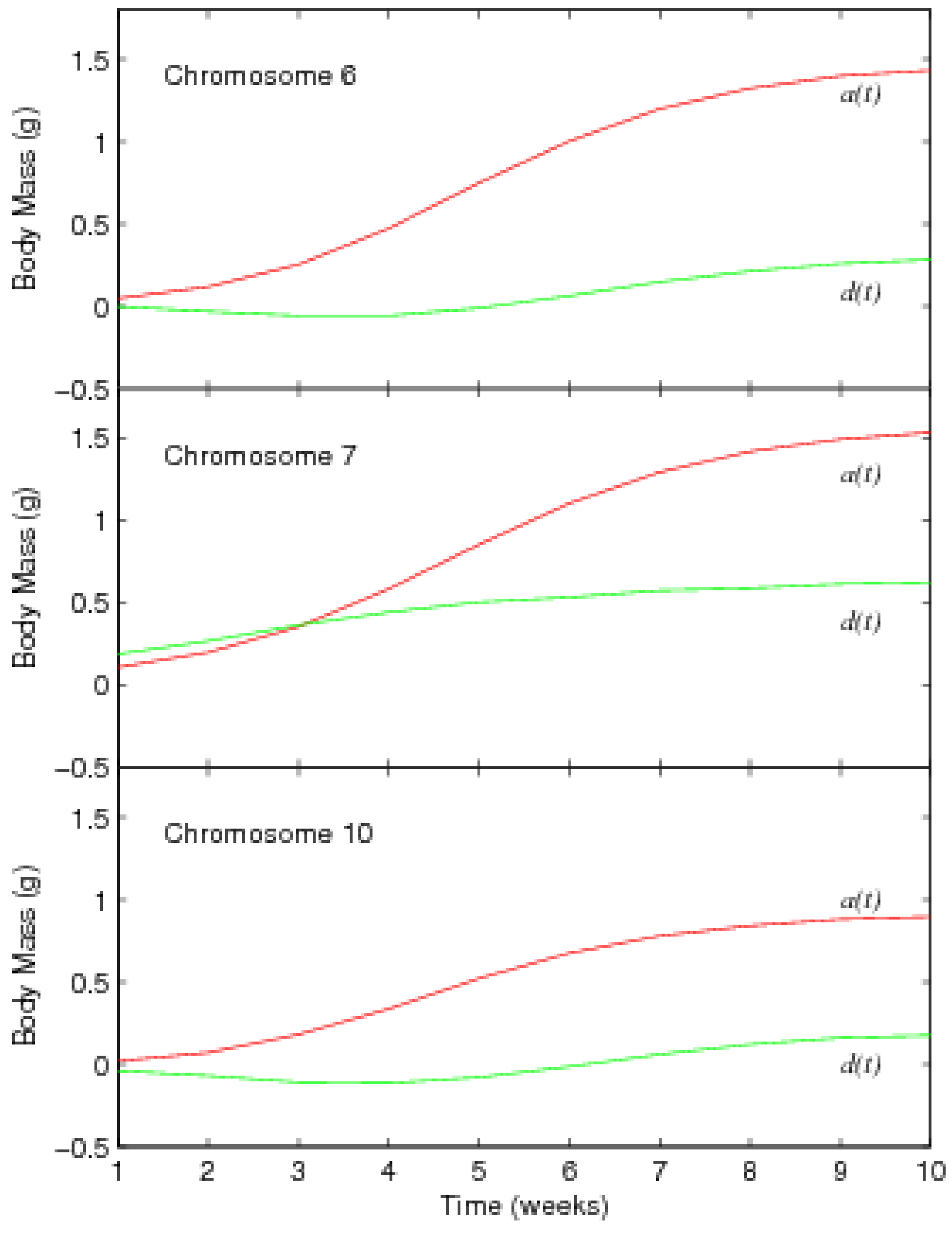
| Chromosome 6 | ||||||
| Location, cM from the first marker 82.68 (67.77, 92.96) | ||||||
| α | 36.09 | (35.20,37.04) | 34.94 | (34.36,35.52) | 33.12 | (32.36,33.93) |
| β | 11.93 | (11.44,12.45) | 11.58 | (11.16,12.03) | 11.07 | (10.65,11.51) |
| γ | 0.65 | (0.64,0.66) | 0.65 | (0.64,0.66) | 0.65 | (0.64,0.67) |
| Chromosome 7 | ||||||
| Location, cM from the first marker 46.84 (38.80,56.02) | ||||||
| α | 36.55 | (35.50, 37.73) | 35.61 | (34.56,36.50) | 33.38 | (32.54,34.33) |
| β | 11.83 | (11.43,12.34) | 11.27 | (10.90,11.73) | 11.25 | (10.76, 11.70) |
| γ | 0.65 | (0.63,0.66) | 0.64 | (0.63,0.65) | 0.65 | (0.63,0.66) |
| Chromosome 10 | ||||||
| Location, cM from the first marker 77.78 (68.75,80.96) | ||||||
| α | 35.41 | (34.33, 36.52) | 34.71 | (33.67,35.70) | 33.59 | (32.61,34.42) |
| β | 11.67 | (11.23,12.19) | 11.47 | (11.23,11.81) | 11.01 | (10.61, 11.44) |
| γ | 0.65 | (0.64,0.66) | 0.64 | (0.63,0.66) | 0.65 | (0.63,0.66) |

4. Monte Carlo Simulation


5. Discussion

| Parameter | ||||||
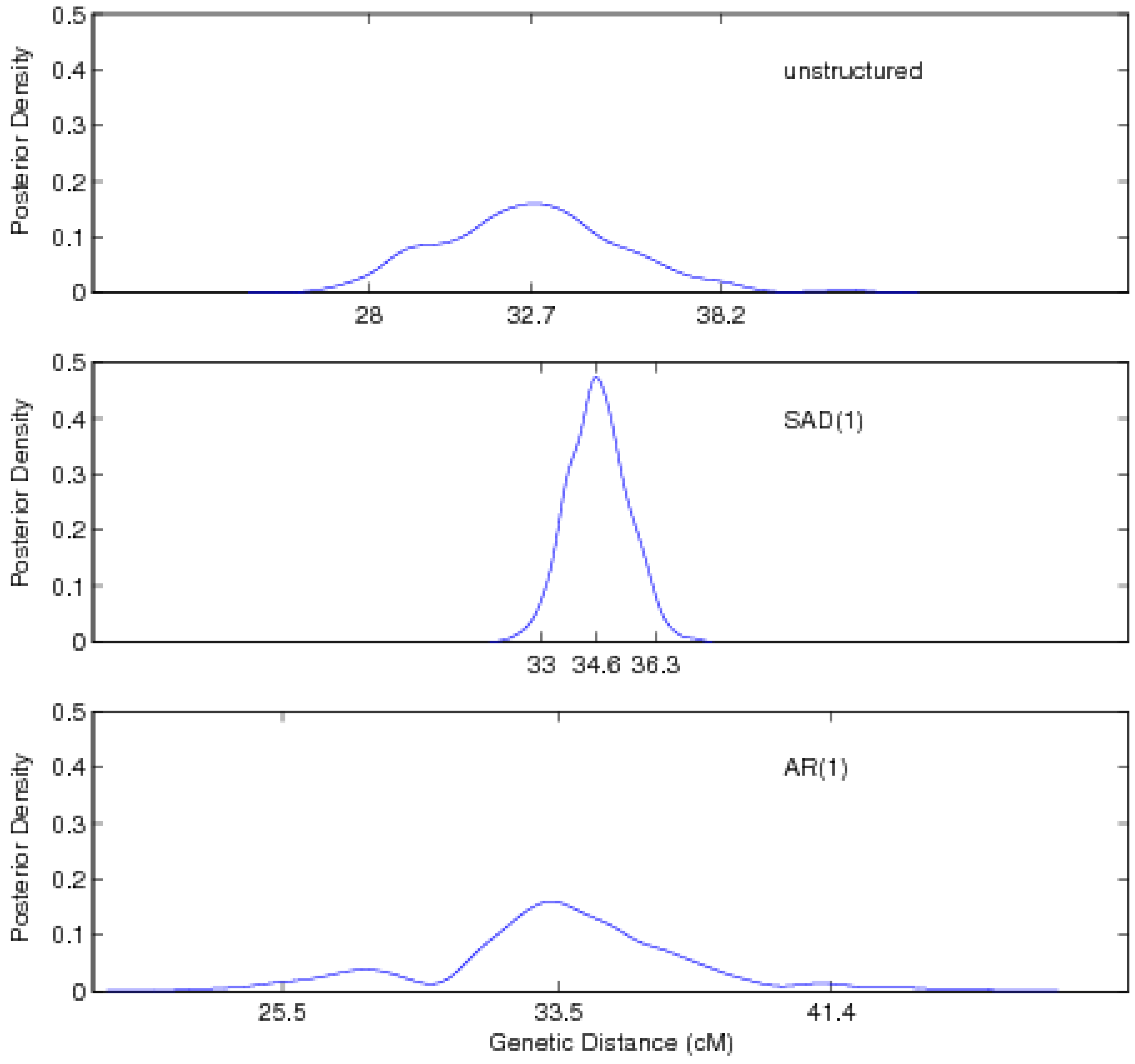
| Unstructured approach | ||||||
| Location | 32.74 (28.02, 38.16) | |||||
| α | 36.67 | (35.81, 37.46) | 36.03 | (35.47, 36.63) | 33.67 | (32.67, 34.31) |
| β | 11.83 | (11.95, 12.64) | 11.22 | (10.97, 11.50) | 11.30 | (10.94, 11.60) |
| γ | 0.66 | (0.64, 0.67) | 0.64 | (0.63, 0.65) | 0.64 | (0.63, 0.66) |
| SAD(1)-structured approach | ||||||
| Location | 34.63 (33.01, 36.30) | |||||
| α | 36.58 | (35.85, 37.36) | 35.88 | (35.37, 36.39) | 33.81 | (33.09, 34.55) |
| β | 12.04 | (11.65, 12.45) | 11.27 | (11.01, 11.54) | 11.46 | (11.09, 11.83) |
| γ | 0.66 | (0.65, 0.67) | 0.64 | (0.63, 0.65) | 0.65 | (0.64, 0.65) |
| AR(1)-structured approach | ||||||
| Location | 33.54 (25.54, 41.39) | |||||
| α | 36.60 | (35.59, 37.66) | 35.57 | (34.88, 36.35) | 33.61 | (32.65, 34.54) |
| β | 12.04 | (11.61, 12.48) | 11.23 | (10.99, 11.56) | 11.42 | (11.05, 11.83) |
| γ | 0.65 | (0.64, 0.66) | 0.63 | (0.62, 0.65) | 0.66 | (0.64, 0.67) |
Appendix A: Estimating (λ,Q,Θ,Σ)
Appendix B. Estimating
Appendix C. Estimating
Appendix D. Alternative Approach for Modeling Σ
- (1)
- Given the current positive-definitive matrix , we set , in the sense that ;
- (2)
- Randomly generate a symmetric p by p matrix T, with elements where ;
- (3)
- Set where ν is generated from ;
- (4)
- Update with an acceptance probability .
Acknowledgements
References and Notes
- Lynch, M; Walsh, B. Genetics and Analysis of Quantitative Traits; Sinauer Associates: Sunderland, MA, USA, 1998. [Google Scholar]
- Paterson, A.H.; Lander, E.S.; Hewitt, J.D.; Peterson, S.; Lincoln, S.E.; Tanksley, S.D. Resolution of quantitative traits into Mendelian factors by using a complete linkage map of restriction fragment length polymorphisms. Nature 1988, 335, 721–726. [Google Scholar] [CrossRef] [PubMed]
- Lander, E.S.; Botstein, D. Mapping Mendelian factors underlying quantitative traits using RFLP linkage maps. Genetics 1989, 121, 185–199. [Google Scholar] [PubMed]
- Zeng, Z.B. Precision mapping of quantitative trait loci. Genetics 1994, 136, 1457–1468. [Google Scholar] [PubMed]
- Weller, J.I. Quantitative Trait Loci Analysis in Animals; CABI Publishing: London, UK, 2001. [Google Scholar]
- Siegmund, D.; Yakir, B. The Statistics of Gene Mapping; Springer: New York, USA, 2007. [Google Scholar]
- Lin, M.; Li, H.; Hou, W.; Johnson, J.; Wu, R.L. Modeling sequence-sequence interactions for drug response. Bioinformatics 2007, 23, 1251–1257. [Google Scholar] [CrossRef] [PubMed]
- Ma, C.X.; Casella, G.; Wu, R.L. Functional mapping of quantitative trait loci underlying the character process: A theoretical framework. Genetics 2002, 161, 1751–1762. [Google Scholar] [PubMed]
- Wu, R.L.; Lin, M. Functional mapping – how to map and study the genetic architecture of dynamic complex traits. Nat. Rev. Genet. 2006, 7, 229–237. [Google Scholar] [CrossRef] [PubMed]
- West, G.B.; Brown, J.H.; Enquist, B.J. A general model for ontogenetic growth. Nature 2001, 413, 628–631. [Google Scholar] [CrossRef] [PubMed]
- Dempster, A.P. Elements of Continuous Multivariate Analysis; Addison-Wesley: Reading, 1969. [Google Scholar]
- Meng, X.L.; Rubin, D.B. Maximum likelihood via the ECM algorithm: A general framework. Biometrika 1993, 80, 267–278. [Google Scholar] [CrossRef]
- Carlin, BP.; Louis, TA. Bayes and Empirical Bayes Methods for Data Analysis; Chapman & Hall: New York, 1996. [Google Scholar]
- Satagopan, J.M.; Yandell, B.S.; Newton, M.A.; Osborn, T.C. A Bayesian approach to detect quantitative trait loci using Markov chain Monte Carlo. Genetics 1996, 144, 805–816. [Google Scholar] [PubMed]
- Sillanpää, M.J.; Arjas, E. Bayesian mapping of multiple quantitative trait loci from incomplete outbred offspring data. Genetics 1999, 151, 1605–1619. [Google Scholar] [PubMed]
- Xu, S. Estimating polygenic effects using markers of the entire genome. Genetics 2003, 163, 789–801. [Google Scholar] [PubMed]
- Yi, N.; Yandell, B.S.; Churchill, G.A.; Allison, D.B.; Eisen, E.J.; Pomp, D. Bayesian model selection for genome-wide epistatic quantitative trait loci analysis. Genetics 2005, 170, 1333–1344. [Google Scholar] [CrossRef] [PubMed]
- Zhang, M.; Montooth, K.L.; Wells, M.T.; Clark, A.G.; Zhang, D. Mapping multiple quantitative trait loci by Bayesian classification. Genetics 2005, 169, 2305–2318. [Google Scholar] [CrossRef] [PubMed]
- Yang, R.Q.; Xu, S. Bayesian shrinkage analysis of quantitative trait loci for dynamic traits. Genetics 2007, 176, 1169–1185. [Google Scholar] [CrossRef] [PubMed]
- Zimmerman, D.L.; Núñez-Antón, V. Parametric modeling of growth curve data: An overview (with discussion). Test 2001, 10, 1–73. [Google Scholar] [CrossRef]
- Diggle, P.J.; Heagerty, P.; Liang, K.Y.; Zeger, S.L. Analysis of Longitudinal Data; Oxford University Press: Oxford, UK, 2002. [Google Scholar]
- Wu, R.L.; Ma, C.M.; Lin, M.; Wang, Z.H.; Casella, G. Functional mapping of growth QTL using a transform-both-sides logistic model. Biometrics 2004, 60, 729–738. [Google Scholar] [CrossRef] [PubMed]
- Carrol, R.J.; Rupert, D. Power transformations when fitting theoretical models to data. J. Am. Stat. Assoc. 1984, 79, 321–328. [Google Scholar] [CrossRef]
- Zhao, W.; Ma, C.M.; Cheverud, J.M.; Wu, R.L. A unifying statistical model for QTL mapping of genotype-sex interaction for developmental trajectories. Physiol. Genomics 2004, 19, 218–227. [Google Scholar] [CrossRef] [PubMed]
- Evans, I.G. Bayesian estimation of parameters of multivariate normal distribution. J. Roy. Statist. Soc. B 1965, 27, 279–283. [Google Scholar]
- Geman, S.; Geman, D. Stochastic relaxation, Gibbs distributions, and the Bayesian restoration of images. IEEE 1984, 6, 721–741. [Google Scholar] [CrossRef]
- Hastings, W.K. Monte Carlo sampling methods using Markov chains and their applications. Biometrika 1970, 57, 397–409. [Google Scholar] [CrossRef]
- Tierney, L. Markov chain for exploring posterior distributions. Ann. Stat. 1994, 22, 1701–1762. [Google Scholar] [CrossRef]
- Fan, J.; Gilbels, I. Local Polynomial Modelling and Its Applications; Chapman & Hall: New York, NY, USA, 1996. [Google Scholar]
- Box, G.; Tao, G. Bayesian Inference in Statistical Analysis; Wiley Interscience: New York, NY, USA, 1973. [Google Scholar]
- Ritter, C.; Tanner, M.A. Facilitating the Gibbs sampler: The Gibbs stopper and Griddy-Gibbs sampler. J. Am. Stat. Assoc. 1992, 87, 861–868. [Google Scholar] [CrossRef]
- Geyer, C. Practical Markov chain Monte Carlo. Stat. Sci. 1992, 7, 473–483. [Google Scholar] [CrossRef]
- Gabriel, K.R. Ante-dependence analysis of an ordered set of variables. Trans. Roy. Soc. Edinb- Earth Sci. 1962, 33, 201–212. [Google Scholar] [CrossRef]
- Jaffrézic, F.; Thompson, R.; Hill, W.R. Structured antedependence models for genetic analysis of repeated measures on multiple quantitative traits. Genet. Res. 2003, 82, 55–65. [Google Scholar] [CrossRef] [PubMed]
- Stephens, M. Bayesian analysis of mixture models with an unknown number of components–An alternative to reversible jump methods. Ann. Stat. 2000, 28, 40–74. [Google Scholar] [CrossRef]
- Cheverud, J.M.; Routman, E.J.; Duarte, FA.M.; van Swinderen, B.; Cothran, K.; Perel, C. Quantitative trait loci for murine growth. Genetics 1996, 142, 1305–1319. [Google Scholar] [PubMed]
- Vaughn, T.T.; Pletscher, L.S.; Peripato, A.; King-Ellison, K.; Adams, E.; Erikson, C.; Cheverud, J.M. Mapping quantitative trait loci for murine growth - A closer look at genetic architecture. Genet. Res. 1999, 74, 313–322. [Google Scholar] [CrossRef] [PubMed]
- Zhao, W.; Chen, Y.Q.; Casella, G.; Cheverud, J.M.; Wu, R.L. A non-stationary model for functional mapping of longitudinal quantitative traits. Bioinformatics 2005, 21, 2469–2477. [Google Scholar] [CrossRef] [PubMed]
- Satagopan, J.M.; Yandell, B.S.; Newton, M.A.; Osborn, T.C. A Bayesian approach to detect quantitative trait loci using Markov chain Monte Carlo. Genetics 1996, 144, 805–816. [Google Scholar] [PubMed]
- Sillanpää, M.J.; Arjas, E. Bayesian mapping of multiple quantitative trait loci from incomplete outbred offspring data. Genetics 1999, 151, 1605–1619. [Google Scholar] [PubMed]
- Raftery, A.E.; Lewis, S. Bayesian Statistics, 4th ED ed; Oxford University Press: Oxford, UK, 1992. [Google Scholar]
- Malosetti Zunin, M.; Visser, R.G.F.; Celis Gamboa, B.C.; van Eeuwijk, F.A. QTL methodology for response curves on the basis of non-linear mixed models, with an illustration to senescence in potato. Theor. Appl. Genet. 2006, 113, 288–300. [Google Scholar] [CrossRef] [PubMed]
- Kao, C.H.; Zeng, Z.B. Modeling epistasis of quantitative trait loci using Cockerham’s model. Genetics 2002, 160, 1243–1261. [Google Scholar] [PubMed]
- Cui, Y.H.; Wu, R.L. Mapping genome-genome epistasis: A multi-dimensional model. Bioinformatics 2005, 21, 2447–2455. [Google Scholar] [CrossRef] [PubMed]
- Green, P.J. Reversible jump Markov chain Monte Carlo computation and Bayesian model determination. Biometrika 1995, 82, 711–732. [Google Scholar] [CrossRef]
- Green, P.J.; Hjort, L.; Richardson, S. Trans-Dimensional Markov Chain Monte Carlo; Oxford University Press: London, UK, 2003. [Google Scholar]
- Brooks, S.P.; Giudici, P. Markov chain Monte Carlo convergence assessment via two-way analysis of variance. J. Comput. Graph. Stat. 2000, 9, 266–276. [Google Scholar]
- Godsill, S.J. On the relationship between MCMC model uncertainty methods. J. Comput. Graph. Stat. 2002, 10, 230–248. [Google Scholar] [CrossRef]
- Dempster, A.P. Elements of Continuous Multivariate Analysis; Addison-Wesley: Reading, MA, USA, 1969. [Google Scholar]
- Stein, C. Estimation of a Covariance Matrix; Rietz Lecture: Atlanta, Georgia, 1975. [Google Scholar]
- Wakefield, J. The Bayesian analysis of population pharmacokinetics models. J. Am. Stat. Assoc. 1969, 91, 62–75. [Google Scholar] [CrossRef]
- Leonardo, T.; Hsu, J.S. Bayesian inference for a covariance matrix. Ann. Stat. 1993, 21, 1–25. [Google Scholar] [CrossRef]
- Yang, R.; Berger, J.O. Estimation of a covariance using the reference prior. Ann, Stat, 1994, 22, 1195–1211. [Google Scholar] [CrossRef]
- Everson, P.J.; Morris, C.N. Inference for multivariate normal hierarchical models. J. Roy. Statist. Soc. B 2000, 62, 399–412. [Google Scholar] [CrossRef]
- Pourahmadi, M. Joint mean-covariance models with applications to longitudinal data: Unconstrained parameterisation. Biometrika 1999, 86, 677–690. [Google Scholar] [CrossRef]
- Bayesian Statistics; Bernardo, J.M.; Berger, J.O.; Dawid, A.P.; Smith, A. F.M. (Eds.) Oxford University Press: Oxford, UK, 1992; p. 3560.
© 2009 by the authors; licensee Molecular Diversity Preservation International, Basel, Switzerland. This article is an open-access article distributed under the terms and conditions of the Creative Commons Attribution license (http://creativecommons.org/licenses/by/3.0/).
Share and Cite
Liu, T.; Wu, R. A Bayesian Algorithm for Functional Mapping of Dynamic Complex Traits. Algorithms 2009, 2, 667-691. https://doi.org/10.3390/a2020667
Liu T, Wu R. A Bayesian Algorithm for Functional Mapping of Dynamic Complex Traits. Algorithms. 2009; 2(2):667-691. https://doi.org/10.3390/a2020667
Chicago/Turabian StyleLiu, Tian, and Rongling Wu. 2009. "A Bayesian Algorithm for Functional Mapping of Dynamic Complex Traits" Algorithms 2, no. 2: 667-691. https://doi.org/10.3390/a2020667
APA StyleLiu, T., & Wu, R. (2009). A Bayesian Algorithm for Functional Mapping of Dynamic Complex Traits. Algorithms, 2(2), 667-691. https://doi.org/10.3390/a2020667