An Improved ABC Algorithm and Its Application in Bearing Fault Diagnosis with EEMD

Abstract

The Ensemble Empirical Mode Decomposition (EEMD) algorithm has been used in bearing fault diagnosis. In order to overcome the blindness in the selection of white noise amplitude coefficient e in EEMD, an improved artificial bee colony algorithm (IABC) is proposed to obtain it adaptively, which providing a new idea for the selection of EEMD parameters. In the improved algorithm, chaos initialization is introduced in the artificial bee colony (ABC) algorithm to insure the diversity of the population and the ergodicity of the population search process. On the other hand, the collecting bees are divided into two parts in the improved algorithm, one part collects the optimal information of the region according to the original algorithm, the other does Levy flight around the current global best solution to improve its global search capabilities. Four standard test functions are used to show the superiority of the proposed method. The application of the IABC and EEMD algorithm in bearing fault diagnosis proves its effectiveness.

1. Introduction

A bearing is an essential part in a rotating machine, which can be easily damaged. At present, the scholars’ research on bearing fault diagnosis can be roughly divided into the following: signal analysis based on vibration [1,2,3,4], monitoring based on temperature [5], and analysis based on acoustic emission [6,7], etc. Among them, the analysis based on vibration signal is the main method for bearing fault diagnosis. In the processing of vibration signals, the commonly used methods are time domain, frequency domain, and time-frequency domain diagnostic methods [8]. The time domain method extracts the time domain characteristics by calculating the time domain parameters of the vibration signal. This method can directly reflect the characteristic information, and the calculation is simple [9]. It can make a preliminary diagnosis on whether the equipment fails, but the fault type and fault location cannot be determined. And a specific judgment on the severity of the failure also cannot be made. The frequency domain diagnosis method analyzes the fault by identifying the difference in the frequency characteristics of the vibration signal between the fault and the normal state. It is based on the theory of Fourier transform [10], which is a global transformation, and unable to perform local analysis for non-stationary and nonlinear signals, moreover it is a pure frequency domain analysis method. There is no resolution in the time domain. Therefore, the frequency domain diagnosis method based on Fourier transform has certain limitations. The time-frequency domain diagnosis method combines the time domain and the frequency domain in two dimensions, so that the signal can be localized simultaneously in the time-frequency domain, which better reflects the local characteristics of the vibration signal [9]. The time-frequency domain diagnosis methods mainly include wavelet transform, wavelet packet transform, Wigner–Vile distribution and empirical mode decomposition (EMD); etc. Their advantages and disadvantages are shown in

Table 1. Comparison of different time-frequency domain methods.

Methods	Advantages	Shortcomings
Wavelet Transform	It has the characteristics of time domain localization and multi resolution. The analysis precision can be adjusted, so that it can accurately locate the short time high frequency and the low frequency component of the signal.	The limited length of the wavelet basis function leads to the energy leakage, which makes the quantitative analysis of the energy-frequency-time distribution become difficult; It does not have adaptive ability, once the basic wavelet is selected, it must be used to analyze all the data to be analyzed.
Wavelet Packet Transform	It can decompose not only the low frequency portion of the signal, but also the high frequency part of the signal, with no redundancy, nor omissions.	The wavelet packet energy, the time-frequency information are not intuitive.
Wiger–Ville	It belongs to bilinear time frequency distribution and has many excellent characteristics, such as high time frequency resolution, energy concentration and time frequency edge characteristics.	Energy density is not guaranteed to be non negative in all time and frequency ranges, and serious cross term interference exists.
EMD	It is especially suitable to analyze nonlinear and non-stationary signal. It breaks through the limitation of the Fourier transform, not only has the characteristics of self adaptation, orthogonality and completeness, but also has the advantages of high efficiency.	The end effect problem, the mode mixing problem, and the decomposition limitation problem exist.

[11].

In Table 1, EMD is a non-stationary signal processing method proposed by Hibert-Huang et al., which can adaptively decompose the local time-varying signals into several intrinsic mode functions (IMF), and reduce the coupling information between signals [7]. Using EMD method to decompose the signal can accurately and effectively grasp the characteristic information of the original data, which is very beneficial to the deeper information mining. However, EMD also has inherent shortcomings, such as endpoint effect problems, mode mixing problems, and decomposition limitations. Therefore, many improved algorithms have been proposed. Ensemble Empirical Mode Decomposition (EEMD) is a major improvement on EMD, which solves the mode mixing problems of EMD [12].

In EEMD algorithm, the Gaussian white noise amplitude coefficient e and the number of EMD decomposition times N should be selected. After adding Gaussian white noise to the original signal x(t), and then starting the EMD decomposition for N times. Average the corresponding EMD decomposition results to get the final IMF [12].

Although EEMD algorithm has achieved good results in improving the mode mixing phenomenon, there are still some shortcomings to be solved. The most serious problem lies in the key parameters setting of the EEMD algorithm, the Gaussian white noise amplitude coefficient $e$ need to be adjusted by experience, and cannot be adaptively gotten according to the characteristics of the signal. Therefore, the processing effect of this method is inevitable different for different signals. The existence of this problem seriously affects the versatility and scope of the EEMD application.

In order to solve the problems of the EEMD method, a large number of researchers have contributed to the selection of the parameters. For example, in literature [13,14], the added white noise was calculated by the high frequency component after EMD decomposition of the original signal, but often due to noise effects and mode mixing, the first IMF cannot accurately reflect the high frequency information. In literature [15], the method of literature [13] was improved by introducing white noise to suppress low-frequency signals and get accurate extraction of high-frequency information. In literature [16], the parameters of the EEMD were determined using signal-to-noise (SNR). In literature [17], the singular value difference spectrum theory is used to extract the composite signal composed of the impact signal and the noise signal, and the probability distribution of the normal distribution function is used to determine the standard deviation of the white noise. In literature [18], white noise with different amplitudes were selected in the interval to perform EEMD decomposition, $e_1$ that minimize the standard deviation of the longitudinal and lateral distributions of the maximum value and $e_2$ that minimize the standard deviation of the longitudinal and the lateral distribution of the minimum value are averaged to get the best $e$. Based on the predecessors, this paper proposes a new idea of using an improved ABC optimization method to select the EEMD parameter e, which reduces the blindness of selecting e when extracting the fault features and improves the applicability of EEMD. The experimental example shows the superiority of the proposed algorithm.

2. The Improved Artificial Bee Colony Algorithm

2.1. Artificial Bee Colony Algorithm

Artificial bee colony algorithm is a kind of swarm intelligence optimization method that was proposed by Karaboga in 2005 [19]. It has few control parameters and good optimization ability. Therefore, it attracts many scholars’ attention. The optimization performance of artificial bee colony is better than that of differential evolution algorithm, genetic algorithm, and particle swarm algorithm [20].

The standard ABC algorithm classifies the bee colony into three kinds by simulating the honey collecting mechanism of actual bees: collecting bees, observing bees, and scouting bees. The goal of the entire colony is to find the source of the most nectar. The collecting bees use the previous honey source information to find a new honey source and share the information with the observing bees. The observing bees waiting in the hive search for a new honey source based on the information shared by the bee. The scouting bee randomly searches for a new valuable source of honey near the hive.

Assuming the solution is a D-dimensional vector, D is the number of the optimized parameters. The specific principle is: First, initialize $S_N$ honey sources, which represent $S_N$ solutions. The numbers of collecting bees and observing bees are also $S_N$. Each collecting bee searches within the neighborhood of the corresponding honey source to find new honey source according to formula (1):

$$X_{ij}^{\prime }=X_{ij}+{\varphi }_{ij}(X_{ij}-X_{kj}),$$

(1)

where: $k\in \left\{1,2,\cdots ,S_N\right\}$, $j\in \left\{1,2,\cdots ,D\right\}$, $k\ne i$; ${\varphi }_{ij}\in [-1,1]$, which is a random number used to control the neighborhood range of $X_{ij}$. The closer to the best solution, the smaller the neighborhood range.

Then the collecting bee compares the new honey source with the old one, using greedy principles to select honey source with high fitness value and shares the information with the observing bee. The observing bees select the honey sources according to the following probability calculation formula:

$$p_i=\frac{F_i}{{\displaystyle \sum _{n=1}^{S_N}{F}_n}},$$

(2)

where, $p_{\mathrm{i}}$ is the probability of observing bee’s choice of honey source and $F_i$ is the fitness value of the ith solution.

Based on $p_{\mathrm{i}}$ and roulette wheel selection, the observing bee selects one solution to update using formula (1) and the greedy criterion is also used to select a better solution with higher fitness. At this stage, only the selected solution can be updated.

If a honey source has not been improved after limit cycles, then the solution will be abandoned. The bee at this position is transformed into a scouting bee, and a new solution is randomly generated according to Equation (3):

$$X_i=X_{\min }+rand(0,1)(X_{\max }-X_{\min }).$$

(3)

2.2. The Specific Improvement of Artificial Bee Colony

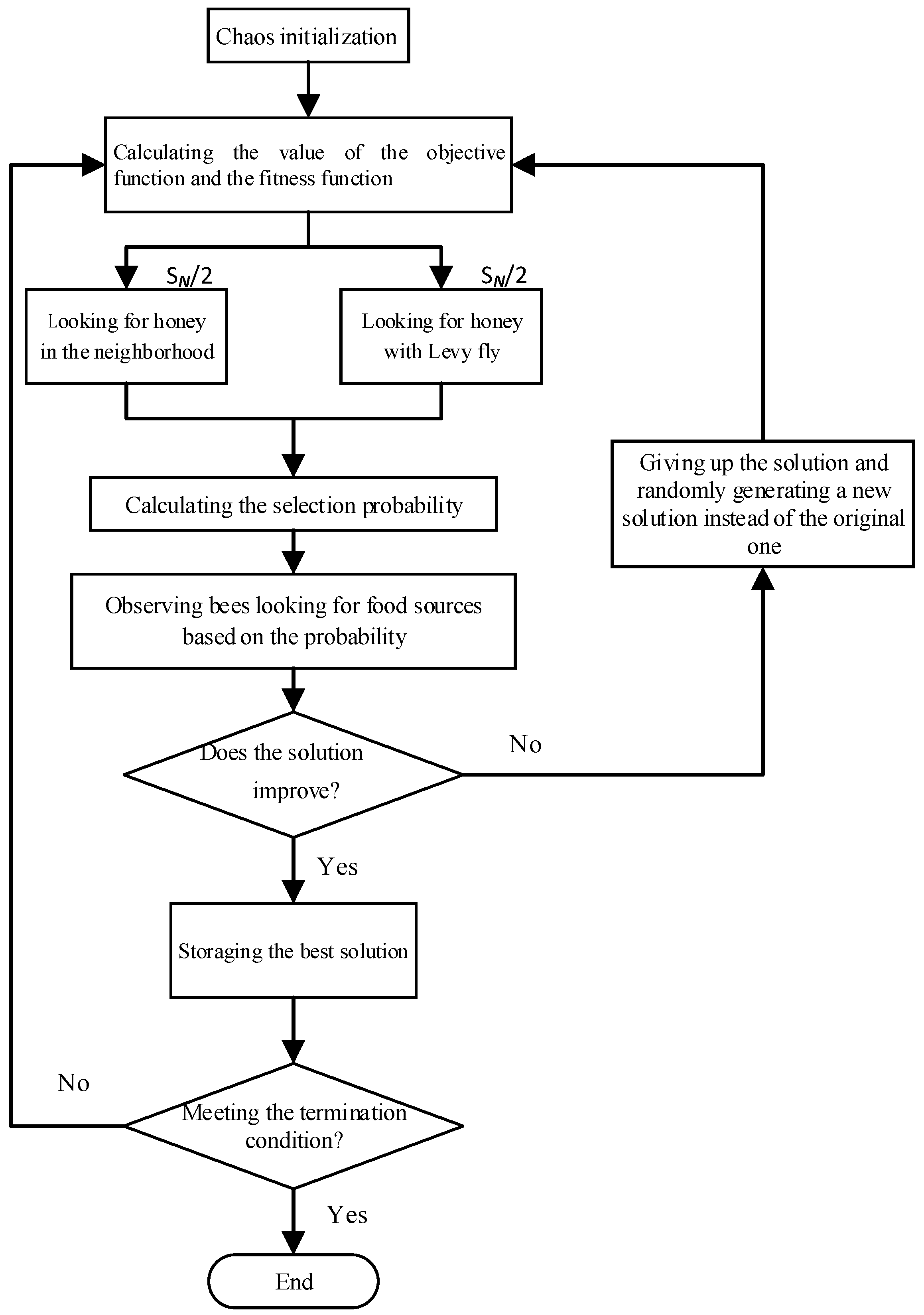
The artificial bee colony algorithm has good optimization ability and is easy to implement, but it also has some shortcomings, such as slow convergence speed and easy to fall into local optimum in the later stage of operation. In order to improve the performance of artificial bee colony algorithm, an improved ABC algorithm based on chaos initialization and Levy flight is proposed to improve the global optimization and the ability to jump out of the local best solution. The specific improvements are as follows.

2.2.1. Chaos Initialization

Chaos seems to be chaotic but has a delicate internal structure, which is a unique and ubiquitous phenomenon in nonlinear systems [21]. Randomness, ergodicity, and regularity are the most typical characteristics of chaos, enabling it to traverse all states within a given range without repeating according to one of its own "laws." Introducing the chaos idea into the artificial bee colony algorithm can prevent it from falling into local optimum and speed up the evolution to some extent. It is proposed to use Logistic chaotic maps to initialize the population. The equations for the Logistic chaotic map are as follows [22]:

$$y_{t+1}=\mu y_t(1-y_t) t=0,1,2,\dots l,$$

(4)

where, $y_t\in (0,1)$ is the chaotic sequence; $\mu$ is the control parameter of the chaotic sequence, its value range is [3.57, 4]; $l$ is the number of iterations of the chaotic sequence.

The specific initialization process is:

①

Sets the iteration number $l$ and the control parameter $\mu$ of the chaotic sequence;

②

The initial chaotic vector $y_0=(y_{01},y_{02},\dots y_{0D})$ is randomly generated, where D is the dimension of the optimization problem;

③

According to Equation (4), a chaotic vector $y_l=(y_{l1},y_{l2},\dots y_{lD})$ is generated;

④

An initial population $X_i=(x_{i1},x_{i2},\dots ,x_{iD})$ is generated according to formula (5);

$$x_{ij}=x_{\min j}+y_{lj}(x_{\max j}-x_{\min j})$$

(5)

⑤

Lets $i=i+1$, if $i$ is greater than the number of populations $S_N$, then ends the process; Otherwise returns to step ②.

After the above steps, a chaotic initial population can be generated.

2.2.2. Levy Flight

Levy flight is a random walk model that describes the anomalous diffusion of nature [23]. Its distribution satisfies the Levy distribution and has long tail characteristics. Since the flying insects such as bees and fruit flies in nature use similar Levy flight methods, several scholars have been inspired by them to introduce Levy flight in the evolution strategy to improve the performance of the algorithm and achieve good results. The specific method is in the bees’ collecting stage of the ABC algorithm, $S_N$ will be divided into two parts, one part collects the optimal information of the region according to the original algorithm, and the other does Levy flight around the current global best solution to improve the global search capabilities. Its update equation is as follows [24]:

$$X_{ij}^{\prime }=X_{ij}+c_1\frac{\varphi u}{{\left|v\right|}^{1/\beta }}(X_{ij}-X_{best}),$$

(6)

where, $c_1$ is the step adjustment factor, usually is taken as 0.01; $u,v$ are random numbers meet standard normal distribution; $\beta$ is a constant that usually satisfies $0<\beta <2$; $\varphi ={\left[\frac{\Gamma (1+\beta )\sin (\pi \beta /2)}{\Gamma (\frac{1+\beta }{2}\beta {.2}^{(\beta -1)/2})}\right]}^{1/\beta }$; $\Gamma$ is the standard Gamma function.

Figure 1 shows the implementation of the improved artificial bee colony algorithm.

2.3. The Verification of the Improved Artificial Bee Colony Algorithm

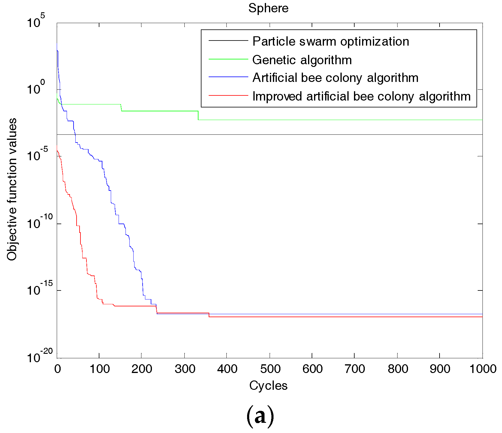
In order to verify the superiority of the improved algorithm, four standard test functions, which are Sphere Model function, Generalized Rosenbrock function, Generalized Griewank function, and Generalized Ackley function are used [25]. The evolution curves of each function are shown in Figure 2. For comparison, the same functions are also optimized by genetic algorithm, particle swarm algorithm and artificial bee colony algorithm. In Equations (7)–(10), $D$ is the dimension of $x$ and let $D=5$ in the four functions.

(1) Sphere Model Function

$$f_1\left(x\right)={\displaystyle \sum _{i=1}^D{x}_i^2} \left(-100\le x_i\le 100\right)min\left(f_1\right)=f_1\left(0,\dots ,0\right)=0$$

(7)

This function is a nonlinear, symmetric single-peak function that can be separated between different dimensions. This function is relatively simple, and it is easier to optimize. Most of the algorithms can achieve good optimization results, so it is usually used to test the optimization accuracy of the algorithm.

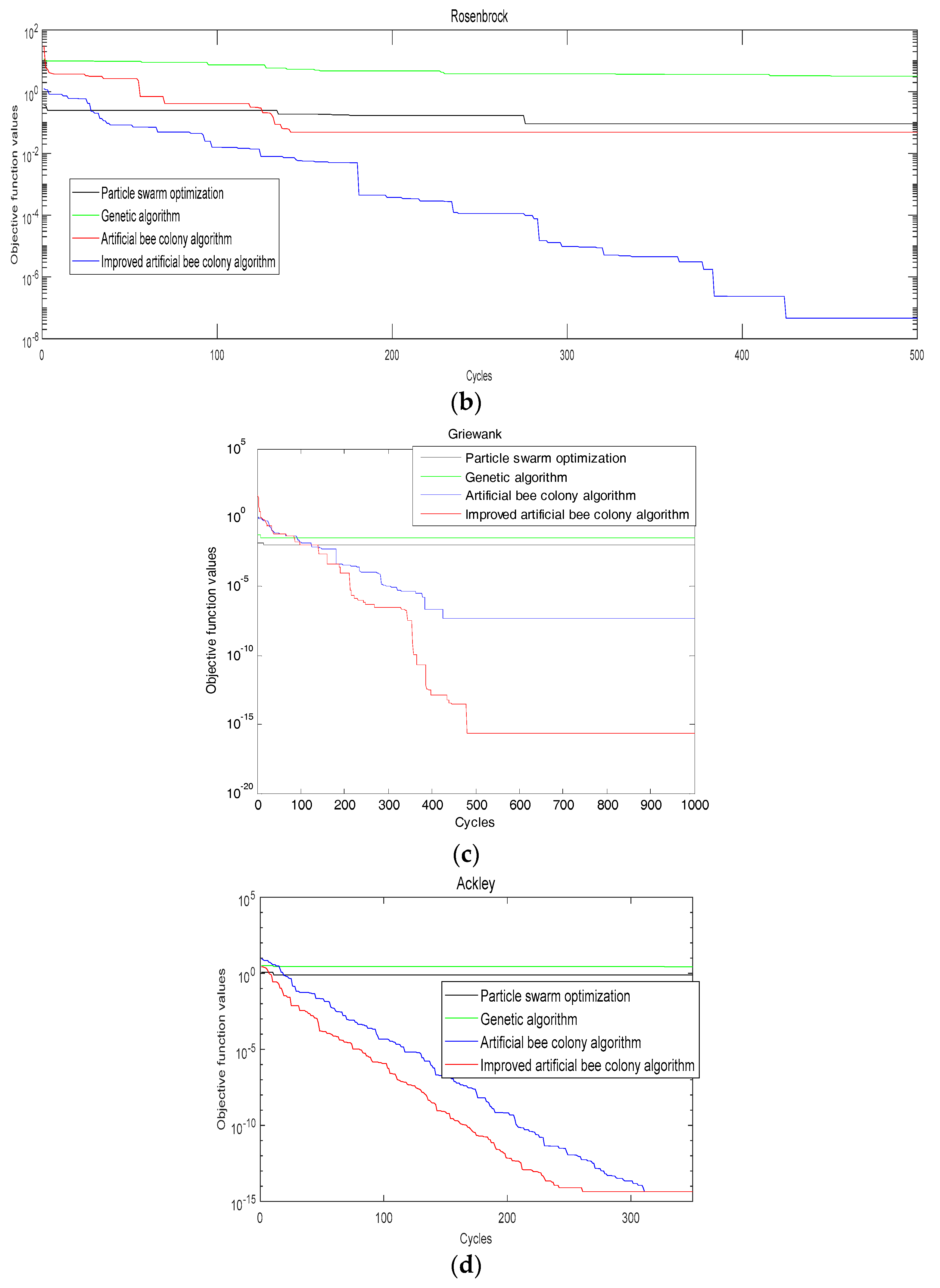
(2) Generalized Rosenbrock Function

$$\begin{gathered} f_2\left(x\right)={\displaystyle \sum _{i=1}^{D-1}\left[100{\left(x_{i+1}-x_i^2\right)}^2+{\left(x_i-1\right)}^2\right]}\left(-30\le x_i\le 30\right) \\ min\left(f_2\right)=f_2\left(0,\dots ,0\right)=0 \end{gathered}$$

(8)

This function is a typical ill-conditioned quadratic function. It is difficult to minimize. There is a narrow valley between its global optimality and reachable local optimum. The best direction from the point on the surface of the valley to the minimum value of the function is almost vertical. Since this function provides very little search information, it is difficult for the algorithm to judge the search direction, and it is difficult to find the global best. Therefore, this function is usually used to measure the execution performance of the algorithm.

(3) Generalized Griewank Function

$$\begin{gathered} f_3\left(x\right)=\frac{1}{4000}{\displaystyle \sum _{i=1}^D{x}_i^2-{\displaystyle \prod _{i=1}^{D}cos\left(\frac{x_i}{\sqrt{i}}\right)}}+1\left(-600\le x_i\le 600\right) \\ min\left(f_3\right)=f_3\left(0,\dots ,0\right)=0 \end{gathered}$$

(9)

This function is a rotating, variable dimension, inseparable multimodal function. The higher the dimension of this function, the easier it is to find the global optimal value. This is because as the dimension increases, the range of local optimum values is getting smaller and smaller. As the quantity changes, there are a large number of local extrema in the entire data distribution of the function. The function is used to detect the ability of an algorithm to jump out of a local.

(4) Generalized Ackley Function

$$\begin{gathered} f_4\left(x\right)=-20exp\left(-0.2\sqrt{\frac{1}{D}{\displaystyle \sum _{i=1}^D{x}_i^2}}\right)-exp\left(\frac{1}{D}{\displaystyle \sum _{i=1}^{D}cos\left(2\pi x_i\right)}\right)+20+e\left(-32\le x_i\le 32\right) \\ min\left(f_4\right)=f_4\left(0,\dots ,0\right)=0 \end{gathered}$$

(10)

This function is a multi-peak function that is rotated, continuous, and inseparable. Since it adjusts the exponential function by the cosine wave, it has many local optimal values, which makes it difficult to find the global optimal value. This function is used to detect the global convergence speed of an algorithm. When the dimension increases, its direction gradient and the direction of advancement are various.

It is found from Figure 2 that using the improved ABC algorithm, a smaller objective function value can be obtained when iterating the same times (bigger than 200) compared with the genetic algorithm, particle swarm algorithm and artificial bee colony algorithm. (The smaller the objective value, the better the decomposition result). The precision and accuracy of searching the best solution are significantly better than that of the other three algorithms. So the improvement has the effect.

3. The Implementation of Optimizing the EEMD Parameters Using Improved Artificial Bee Colony Algorithm

According to the experience, the decomposition number N required by EEMD is closely related to the white noise amplitude coefficient e, the intrinsic relationship is shown in Equation (11) [17].

$$N={\left(\frac{e}{\epsilon }\right)}^2,$$

(11)

where, $\epsilon$ is the decomposition error. Generally, $e=0.2$, $\epsilon =2\%$, and $N=100$ [17]. In order to reduce the error caused by the addition of noise, according to literature [18], the minimum value of N is 20. Therefore, N is taken as 20 in this paper, the white noise amplitude coefficient e will be optimized using improved artificial bee colony algorithm.

The purpose of adding white noise in EEMD is to smooth the abnormal events to make the distribution of signal extreme points more uniform, yet the influence of different e on the distribution uniformity of extreme points is different.

The amplitude difference and the spacing (interval points) of the adjacent points of the maximum (minimum) sequence respectively reflect the longitudinal and the lateral distribution of the maximum (minimum). When the amplitude difference and the spacing of adjacent points of the maximum (minimum) sequence do not change too much, which means when the fluctuation is small, the distribution of the maximum (minimum) is uniform.

The degree of the fluctuation of the maximum (minimum) sequence can be measured by the standard deviation. If the standard deviation is small, the fluctuation is small, and vice versa. According to literature [18], in order to make the distribution of the maximum (minimum) sequence more uniform, the amplitude difference and the spacing fluctuation of the adjacent points of the maximum (minimum) sequence should be smaller. So, for different e, calculating the standard deviation std1_max (stdl_min) of the amplitude difference and the standard deviation std2_max (std2_min) of the spacing of the adjacent points of the maximum (minimum) sequence, taking into account the two variation together, the multiplication std_max (std_min) can be gotten. When std_max and std_min are the smallest, the vertical and horizontal fluctuations of the signal maximum (minimum) sequence are the smallest, which means the distribution is the most uniform. Std_max and std_min are shown in Equations (12) and (13). In the optimization process, the objective function is selected as (std_max) + (std_min), and the white noise amplitude coefficient e which minimizes the objective function is selected as the best one.

The specific steps for optimizing the EEMD parameters using the improved artificial bee colony algorithm are:

• Sets the number of the honey source $S_N$ to be 20, the maximum iteration number to be 10, the range of e to be [0.01, 0.5], limit to be 100, $\mu =4$, $l=10$, initialize the honey source using Logistic chaotic maps according to the steps in Section 2.2;
• Calculates the value of the objective function and the fitness function for each honey source (solution);
• One part of the collecting bees ($S_N/2$) searches the honey source neighborhood according to Equation (1) and the other part of the collecting bees searches around the current global best solution with Levy flight according to Equation (6)
• Calculates the objective function value and the fitness function value of the mutated honey source, selects the honey source with better fitness and updates the current honey source information;
• Observing bees select the honey source with higher fitness according to the probability calculated through Equation (2), and perform neighborhood searching according to Equation (1). Calculates the objective function value and fitness function value of the honey source after mutation, and updates the relevant information of the current honey source;
• Finds the honey source that has not been updated at most consecutive times. If the number of consecutive times is greater than the limit, then the honey source is reinitialized by the scouting bees according to Equation (3), and turns to step (2). Otherwise records the best solution of this time.
• Judges whether the maximum number of iterations is reached, if not, then turns to step (2), otherwise, outputs the best solution.

  $$\mathrm{std}\_\max =\sqrt{\frac{1}{N_1-1}{\displaystyle \sum _{i=1}^{N_1-1}\left(\left|x_{1i+1}-x_{1i}\right|-u_1\right)}}\times \sqrt{\frac{1}{N_1-1}{\displaystyle \sum _{i=1}^{N_1-1}\left(\left|y_{1i+1}-y_{1i}\right|-u_1^{\prime }\right)}}$$

  (12)

  $$\mathrm{std}\_\min =\sqrt{\frac{1}{N_2-1}{\displaystyle \sum _{i=1}^{N_2-1}\left(\left|x_{2i+1}-x_{2i}\right|-u_2\right)}}\times \sqrt{\frac{1}{N_2-1}{\displaystyle \sum _{i=1}^{N_2-1}\left(\left|y_{2i+1}-y_{2i}\right|-u_2^{\prime }\right)}}$$

  (13)

where, $N_1$, $N_2$ are the numbers of points of extr_max($x_1$, $y_1$) and extr_min($x_2$, $y_2$); $u_1$ $u_1^{\prime }$, $u_2$, $u_2^{\prime }$ are the average of the amplitudes difference and the number of intervals of extr_max($x_1$, $y_1$) and extr_min($x_2$, $y_2$), respectively.

4. Application Example

In order to illustrate the accuracy and superiority of the proposed algorithm, the public bearing data set of the University of Cincinnati was first used to verify the effectiveness of the algorithm.

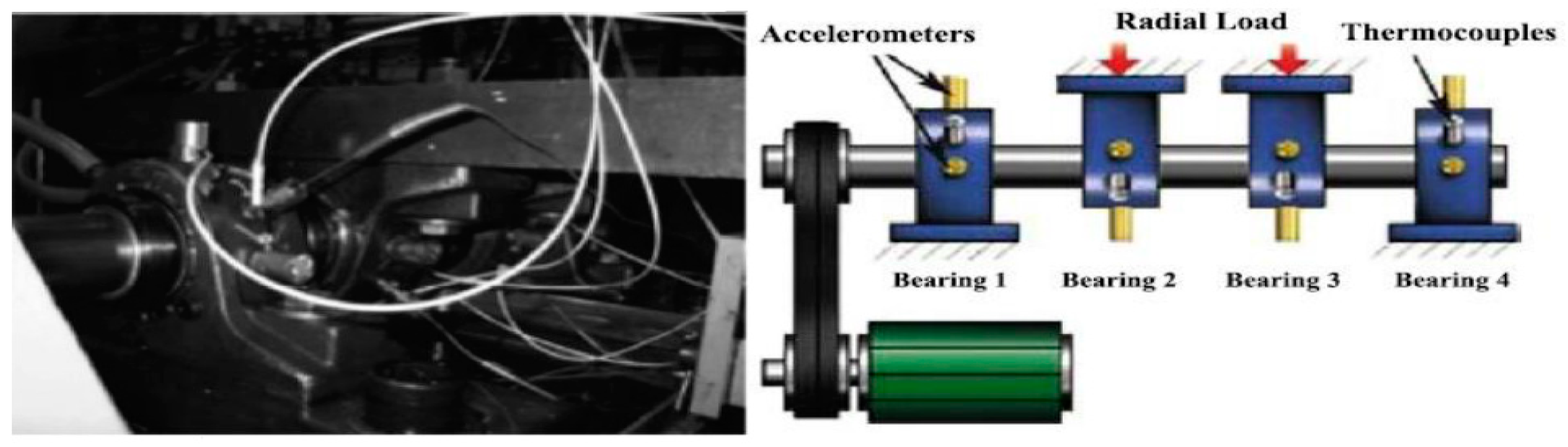
Figure 3 is the corresponding experimental setup. Selecting the outer ring fault data of bearing 1 to be analyzed. According to the parameters of the experimental device ($z=16$, $d=0.331\mathrm{in}.$, $D=2.815\mathrm{in}.$, $\alpha ={15.17}^{\circ }$, $n=2000\mathrm{rpm}$) and formula (14), it can be calculated that the fault frequency of the outer ring is:$f_{ep}=236.4\mathrm{Hz}$.

$$f_{ep}=\frac{z}{2}•\frac{n}{60}\left(1-\frac{d}{D}\cos \alpha \right)$$

(14)

where, $z$ is the number of rolling bodies; $d$ is the diameter of the rolling body; $D$ is the bearing pitch; $\alpha$ is contact angle; and $n$ is the rotation speed.

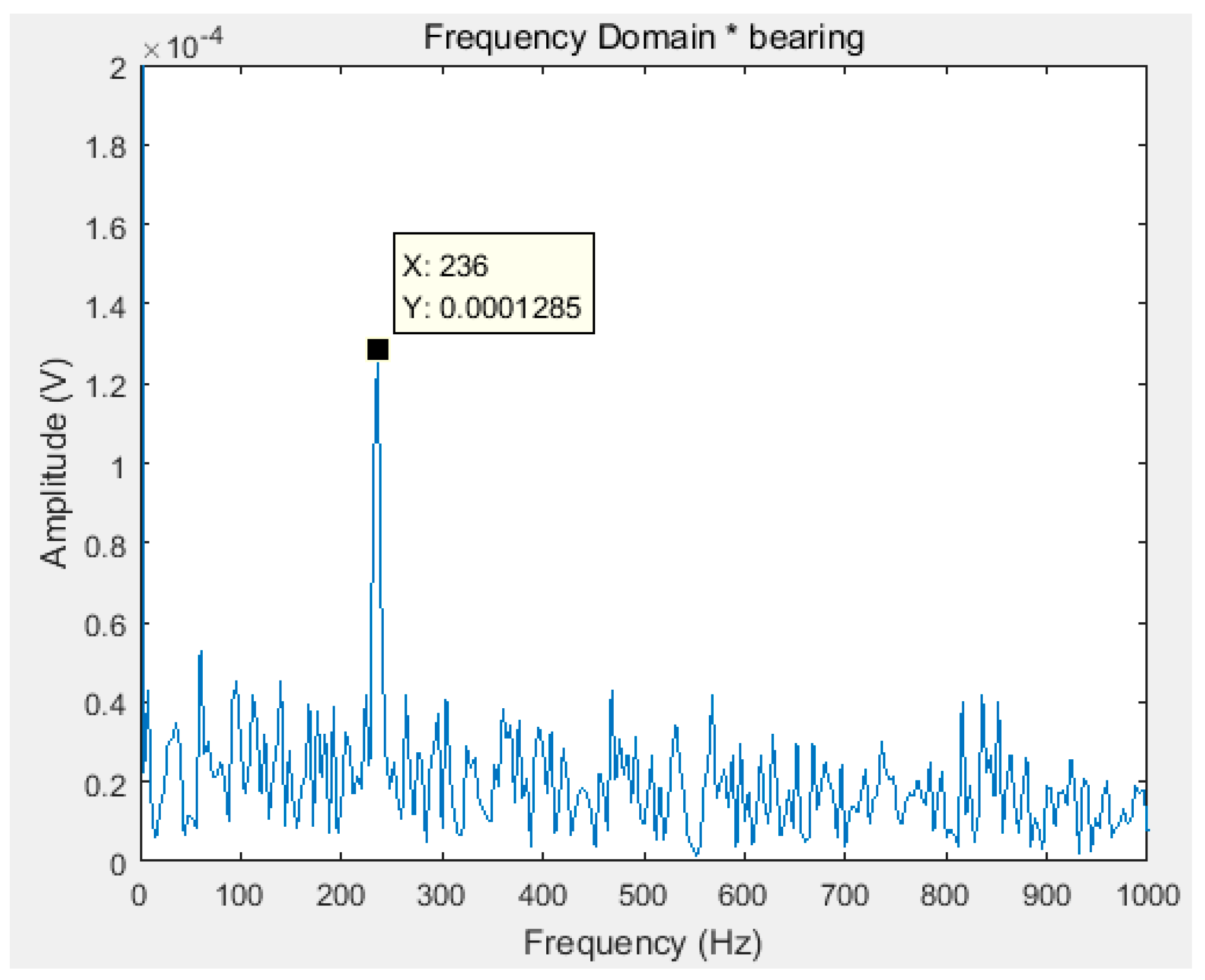
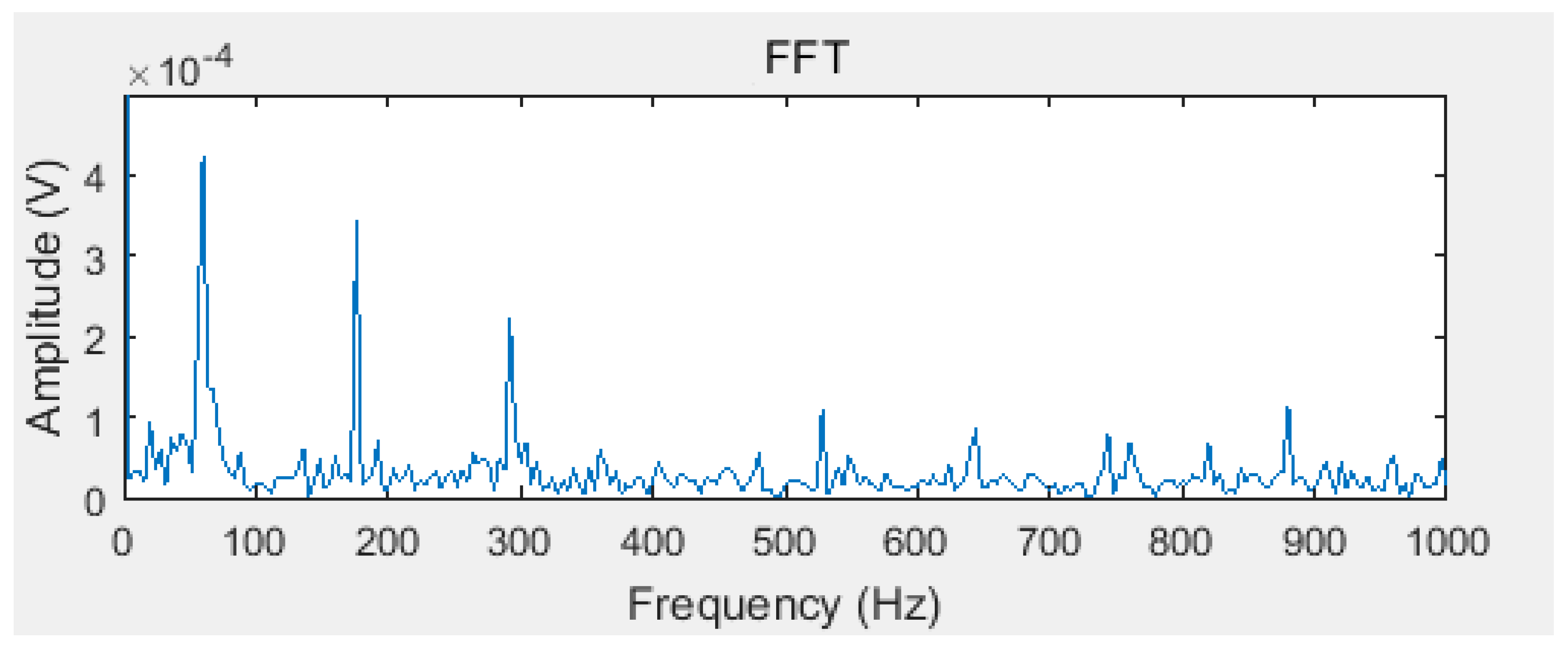
Taking (std_max) + (std_min), which are shown in the Equations (12) and (13), as the objective function, Equation (15) as the fitness function, optimizing the white noise amplitude coefficient according to Section 3 to get $e=0.342819$. According to literature [18], the minimum value of N is 20. After the EEMD of the original signal, 13 IMF components can be gotten. Figure 4 is a Fourier transform spectrum of the maximum kurtosis IMF component obtained by the proposed algorithm in this paper. In order to show the superiority of the decomposition, the Fourier transform spectrum of the original signal is shown in Figure 5.

$$fitness=1/(1+f(\mathrm{obj})),$$

(15)

where $f(\mathrm{obj})$ is the objective function.

It can be seen that the fault frequency can be easily found in the IMF of EEMD optimized by the improved ABC proposed in this paper. However, in the Fourier transform spectrum of the original signal (Figure 5), the fault frequency cannot be found.

In order to illustrate the superiority of the proposed algorithm, the orthogonality of the IMF components (index of orthogonality, referred as IO) and the time indicators are used in this paper. The IO calculation formula is shown in Equation (16) [26], the smaller the value, the higher the accuracy. The specific values of the indicators after decomposition using EMD, experienced EEMD, EEMD of literature [13,16,18], EEMD optimized by ABC and EEMD optimized by IABC are listed in

Table 2. Indicator values after decomposition by different methods.

Items	EMD	EEMD (experienced)	EEMD (literature 13)	EEMD (literature 16)	EEMD (literature 18)	EEMD (ABC)	EEMD (IABC)
e	0	0.2	0.1428	0.5119	0.33	0.321838	0.342819
N	1	100	20	20	20	20	20
IO	0.0568	0.0277	0.0213	0.0264	0.0176	0.0119	0.0086
Running time(s)	0.334980	18.600744	3.555455	3.587991	4.605549	3.744001	3.539447

.

$$IO={\displaystyle \sum _{t=0}^T\left({\displaystyle \sum _{i=1}^{n+1}{\displaystyle \sum _{j=1}^{n+1}{c}_i\left(t\right)c_j\left(t\right)/x^2\left(t\right)}}\right)}\left(i\ne j\right),$$

(16)

where T is the total length of the signal.

It can be seen from Table 2 that the proposed EEMD, whose amplitude parameter $e$ was obtained through the improved artificial bee colony optimization algorithm, has a better decomposition effect after a small number of decompositions.

5. Conclusions

Bearing fault diagnosis is an important topic in these years. EEMD is a time-frequency domain diagnosis method usually used in recent years. In the paper, an improved artificial bee colony algorithm is proposed first. Its superiority is proved by four standard test functions. Then it is used to select the important white noise amplitude coefficient parameter e in EEMD based on its influence on the uniformity of the signal extreme point distribution. The application example demonstrates the effectiveness of the method.

Using the improved artificial bee colony algorithm to find the parameters of EEMD is a new method. It is different from the previous methods, such as designating according to experience, calculating high-frequency components or calculating through finite points of $e$ etc. It is a more intelligent parameter optimization algorithm. At present, this method is only used in the fault diagnosis of bearings. It is hoped that in the subsequent research, its application will be further expanded to get the feature extraction in various fields.

References

- Xiao, Y.C.; Wang, Y.J.; Ding, Z.T. The Application of Heterogeneous Information Fusion in Misalignment Fault Diagnosis of Wind Turbines. Energies 2018, 11, 1655. [Google Scholar] [CrossRef]
- Xu, Y.G.; Zhang, K.; Ma, C.Y.; Li, X.Q.; Zhang, J.Y. An Improved Empirical Wavelet Transform and Its Applications in Rolling Bearing Fault Diagnosis. Appl. Sci. 2018, 8, 2352. [Google Scholar] [CrossRef]
- Tang, G.; Pang, B. Application of ITT transform in fault diagnosis of wind turbine rolling bearing. Electr. Power Autom. Equip. 2017, 37, 83–89. (in Chinese). [Google Scholar]
- Hasan, M.J.; Kim, J.M. Bearing Fault Diagnosis under Variable Rotational Speeds Using Stockwell Transform-Based Vibration Imaging and Transfer Learning. Appl. Sci. 2018, 8, 2357. [Google Scholar] [CrossRef]
- Zhang, X.T.; Yan, S.T.; Zhou, X.Q.; Zhao, H.S. Early stage failure forecast method for main bearing of wind turbine based on state monitoring. Guangdong Electr. Power 2012, 25, 6–10. (in Chinese). [Google Scholar]
- Li, N.; Wei, P.; Mo, H.; Mei, S.K.; Li, M. Bearing state monitoring using a novel fiber bragg grating acoustic emission technique. J. Vib. Shock 2015, 34, 172–177. [Google Scholar]
- Li, R.Y.; He, D. Rotational machine health monitoring and fault detection using EMD-based acoustic emission feature quantification. IEEE Trans. Instrum. Meas. 2012, 61, 990–1001. [Google Scholar] [CrossRef]
- Lang, L. Research on Fault Diagnosis of Wind Turbine Bearing Based on Vibration Signal; North China Electric Power University: Baoding, China, 2017. [Google Scholar]
- Xiao, Y.C.; Wang, Y.J.; Mu, H.; Kang, N. Research on Misalignment Fault Isolation of Wind Turbines Based on the Mixed-Domain Features. Algorithms 2017, 10, 67. [Google Scholar] [CrossRef]
- Yuan, Z.J.; Huang, X.; Yuan, L.F. An Application of Fourier Transforms in Nonparametric Statistics. Math. Pract. Theory 2018, 14, 312–315. [Google Scholar]
- Xiao, Y.C.; Kang, N.; Hong, Y.; Zhang, G.J. Misalignment Fault Diagnosis of DFWT Based on IEMD Energy Entropy and PSO-SVM. Entropy 2017, 19, 6. [Google Scholar] [CrossRef]
- Wu, Z.; Huang, N.E. Ensemble empirical mode decomposition: a noise assisted data analysis method. Adv. Adapt. Data Anal. 2009, 1, 1–41. [Google Scholar] [CrossRef]
- Chen, L.; Tang, G.S.; Zi, Y.Y.; Feng, Z.N.; Li, K. Application of Adaptive Ensemble Empirical Mode Decomposition Method to Electrocardiogram Signal Processing. J. Data Acquis. Process. 2011, 26, 361–366. [Google Scholar]
- Yue, X.F.; Shao, H.H. Fault diagnosis of rolling element bearing based on improved ensemble empirical mode decomposition. Manuf. Autom. 2015, 37, 80–83. [Google Scholar]
- He, X.; Wang, H.L.; Jiang, W.; Wang, L. Improved Adaptive EEMD Method and Its Application. J. Syst. Simul. 2014, 26, 869–873. [Google Scholar]
- Wei, Y.H.; Wang, M.H.; Lin, M.J.; Tian, P. A Technology on Rolling Bearings Fault Feature Extraction Based on Improved EEMD. Modul. Mach. Tool Autom. Manuf. Tech. 2015, 1, 87–90. [Google Scholar]
- Zhou, W.L. Diagnosis and Research of Wind Turbine Planetary Gearbox Faults Based on adaptivity EEMD; Shanghai Electric Power College: Shanghai, China, 2017. [Google Scholar]
- Chen, R.X.; Tang, B.P.; Yang, L.X.; Zhou, G.W. An EEMD-Feature Extraction Method of Mechanical Fault Based on Adaptive Parameter Optimum. J. Vib. Meas. Diagn. 2014, 34, 1065–1071. [Google Scholar]
- Karaboga, D. An Idea Based on HoneyBee Swarm for Numerical Optimization, Technical Report-TR06; Erciyes University: Kayseri, Turkey, 2005. [Google Scholar]
- Karaboga, D.; Akay, B. A Comparative Study of Artificial Bee Colony Algorithm. Appl. Math. Comput. 2009, 214, 108–132. [Google Scholar]
- Dittrich, T. Quantum Chaos and Quantum Randomness—Paradigms of Entropy Production on the Smallest Scales. Entropy 2019, 21, 286. [Google Scholar] [CrossRef]
- Cai, D.; Ji, X.Y.; Shi, H.; Pan, J.M. Method for improving piecewise Logistic chaotic map and its performance analysis. J. Nanjing Univ. 2016, 52, 809–815. [Google Scholar]
- Pang, B.; Song, Y.; Zhang, C.J.; Wang, H.L.; Yang, R.T. A Modified Artificial Bee Colony Algorithm Based on the Self-Learning Mechanism. Algorithms 2018, 11, 78. [Google Scholar] [CrossRef]
- Xue, H.R.; Zhang, K.H.; Li, B.; Peng, C.H. Fault diagnosis of transformer based on the cuckoo search and support vector machine. Power Syst. Prot. Control 2015, 43, 8–13. [Google Scholar]
- Zhang, S.S. A Study on Gear Fault Diagnosis Technology Based on Support Vector Machine Optimized by Bee Colony Algorithm; Northeast Petroleum University: Daqing, China, 2015. [Google Scholar]
- Huang, N.E.; Shen, Z.; Long, S.R. The empirical mode decomposition and the Hilbert spectrum for nonlinear and non-stationary time series analysis. Proc. R. Soc. Lond. 1998, 454, 903–995. [Google Scholar] [CrossRef]
Figure 1.
Principle of the Improved Artificial Bee Colony Algorithm.
Figure 2.
Evolution curve of each function. (a) Sphere function; (b) Rosenbrock function; (c) Griewank function; and (d) Ackley function.
Figure 3.
The experimental setup.
Figure 4.
The Fourier transform spectrum of the IMF component with the maximum kurtosis.
Figure 5.
The Fourier transform spectrum of original signal.