Optimized Deep Convolutional Neural Networks for Identification of Macular Diseases from Optical Coherence Tomography Images

Abstract

Finetuning pre-trained deep neural networks (DNN) delicately designed for large-scale natural images may not be suitable for medical images due to the intrinsic difference between the datasets. We propose a strategy to modify DNNs, which improves their performance on retinal optical coherence tomography (OCT) images. Deep features of pre-trained DNN are high-level features of natural images. These features harm the training of transfer learning. Our strategy is to remove some deep convolutional layers of the state-of-the-art pre-trained networks: GoogLeNet, ResNet and DenseNet. We try to find the optimized deep neural networks on small-scale and large-scale OCT datasets, respectively, in our experiments. Results show that optimized deep neural networks not only reduce computational burden, but also improve classification accuracy.

1. Introduction

The retina in human eyes receives the focused light by the lens, and converts it into neural signals. The main sensory region for this purpose is the macula which is located in the central part of a retina. The macula is responsible for the central, high-resolution, color vision that is possible in good light. The retina processes the information gathered by the macula, and sends it to the brain via the optic nerve for visual recognition.

Macular health can be affected by a number of pathologies, including age-related macular degeneration (AMD) and diabetic macular edema (DME). They account for the majority of irreversible vision loss subjects in developed and developing countries [1,2,3]. In the case of DME fluid is accumulated [4] and in the case of dry AMD drusen is deposited resulting in geographic atrophy, thereby incurring the deformation of retinal layers [5,6]. Without appropriate treatment, patients of dry AMD may develop choroidal neovascularization (CNV), a severe blinding form of advanced AMD (i.e. wet AMD). In the case of CNV, new blood vessels are created in the choroid layer of the eye.

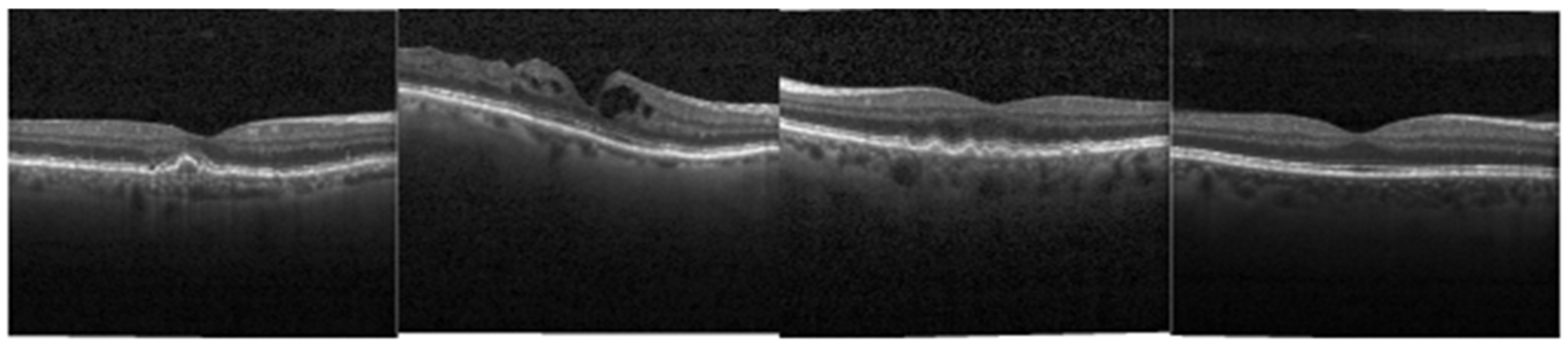
In ophthalmology, one of the most commonly used integral imaging techniques is spectral domain optical coherence tomography (SD-OCT), with approximately 30 million OCT scans performed each year worldwide [7]. OCT is a non-invasive imaging technique, which captures cross-sectional images at microscopic resolution of biological tissues [8]. By providing a clear cross-sectional representation of the retinal pathology in these conditions (Figure 1), OCT is critical to the early identification and treatment of retinal pathologies today. Examples in Figure 1 are picked from a public dataset provided by [9].

Since OCT image interpretation is time-consuming and tedious for ophthalmologists, different computer-aided diagnosis (CAD) systems for semi/fully automatic analysis of OCT data have been developed in the past decade. We now briefly discuss a number of related works on the topic of OCT data classification. In 2011, Liu et al. proposed a methodology for detecting macular pathologies (including AMD and DME) in fovea slices of OCT images, in which they used local binary patterns (LBP) and represented images using a multi-scale spatial pyramid (SP) followed by a principal component analysis (PCA) for dimension reduction [10]. In 2012, Zheng et al. and Hijazi et al. proposed methods for representing images based on a graph [11,12]. In 2014 Shinivasan et al. presented a method for classifying AMD, DME and healthy C-scans using multi-scale histogram of gradients (HoG) features and a support vector machine (SVM) classifier [13]. In 2017, Sun et al. proposed a classification method based on techniques of scale-invariant feature transform (SIFT), sparse coding (SC), dictionary learning (K-SVD), multi-scale max pooling and linear SVM [14].

In recent years, deep neural networks (DNNs) have outperformed many traditional techniques on the large-scale ImageNet dataset [15]. Researchers designed many networks to obtain high accuracy and reduce parameters, such as AlexNet [16] in 2012, VGGnet [17] in 2014, GoogLeNet [18,19] in 2015, ResNet [20] in 2016 and DenseNet [21] in 2017. The outstanding performance of DNN inspires scholars to apply them on medical images [22,23].

To our best knowledge, there are three kinds of methods to apply DNN on medical images. The first one, also the most straightforward, is to initialize randomly all the layers of a DNN and train the DNN on medical datasets. This method requires large-scale medical datasets, which is not always available in real world. The second method utilizes pre-trained DNN as feature extractor, extracts features of medical images and classifies them with softmax dense layer, SVM, random forest (RF) or other statistic classifier. This method is efficient since no training of the DNN is required. The last one is to finetune the DNN pre-trained on ImageNet dataset using medical datasets. Some experiments have been conducted to compare these three methods. Abdolmanafi et al. discusses the performance of three state-of-the-art networks (AlexNet, VGG-19 and Inception-v3) on characterization of coronary artery pathological formations from OCT imaging. In the experiment of finetuning, classification layers are adapted to their data set, and in the experiments of feature extraction, features are extracted before the last fully connected layer right before the classification layer (pre-trained AlexNet, VGG-19) or before the last depth concatenation layer (mixed10 layer in pre-trained Inception-v3). Experimental results show that finetuning method outperforms the feature extraction method with RF as classifier [24]. Karri et al. compares training GoogLeNet from scratch and finetuning pre-trained GoogLeNet on retinal OCT dataset, and their results show that fine-tuned DNN performs better both in convergence speed and classification accuracy [25]. Extensive experiments based on 4 distinct medical-imaging applications from Tajbakhsh et al. demonstrate that deeply fine-tuned convolutional neural networks (CNN) are useful for medical image analysis, performing as well as fully trained CNNs and even outperforming the latter when limited training data are available. They also observed that the required level of finetuning differs from one application to another, which means that the strategy of finetuning still remains an open question [26].

Since pre-trained networks are trained on 1.2 million natural images of 1000 classes from ImageNet, the filters learned may not be suitable for the retinal OCT classification. To further explore the filters and improve performance of pre-trained DNNs, some visualization techniques of DNN are developed [27,28]. Their visualizations show the increase in complexity and variation on higher layers, comprised of simpler components from lower layers. The variation of patterns increases with increasing layer number, indicating that increasingly invariant representations are learned. Inspired by these results, we remove the deeper layers of the pre-trained DNNs such that in the process of transfer learning, the DNNs classify OCT images with the help of low-level features of natural images, without the interference of high-level features. We investigate the performance on ImageNet dataset of some modern DNNs such as VGGNet, GoogLeNet, ResNet, DenseNet, MobileNet [29,30] and NASNet [31]. In consideration of the balance between classification accuracy and computational efficiency, we choose Inception-v3, ResNet50 and DenseNet121 as base networks in our experiments.

Our work is organized as follows. First, the architectures of modified DNNs are illustrated in Section 2. Datasets, experiments and results are presented in Section 3. Finally, this study is concluded in Section 4.

2. Architectures of the Modified Deep Neural Networks (DNNs)

In this section, we briefly discuss the parameters, architecture and sub-networks of the three modern DNNs (Inception-v3, ResNet50 and DenseNet121).

2.1. Sub-Networks of Inception-v3

Inception-v3 is a classical deep network. Its architecture is shown in Figure 2. The network is composed of 11 Inception modules of five kinds in total. Each module is designed by experts with convolutional layer, activation layer, pooling layer and batch normalization layer. In the Inception-v3 model, these modules are concatenated to achieve maximal feature extraction.

Inception modules adopt the idea of multi-scale. Each module has multiple branches with different sizes of kernels (1 × 1, 3 × 3, 5 × 5 and 7 × 7). These filters extract and concatenate different scale of feature maps and send the combination to the next stage; 1 × 1 convolutions in each inception module is used for dimensionality reduction before applying computationally expensive 3 × 3 and 5 × 5 convolutions. Factorization of 5 × 5, 7 × 7 convolution into smaller convolutions (3 × 3) or asymmetric convolutions (1 × 7, 7 × 1) reduces the number of DNN parameters.

After removing some deep Inception modules and the classification layers (global average pooling layer and last dense layer with 1000 outputs), we add a set of classification layers (a global average pooling layer, a dense layer with 3 or 4 outputs in our experiments) adapted to our datasets to the new network graph. Sub-networks are named after their last depth concatenation layers; whose names are consistent with that in the Keras implementation (the python deep learning library) [32]. For example, “mixed10” represents the sub-network removing no module; “Mixed9” represents the sub-network removing Inception E2 module; “Mixed8” represents the sub-network removing Inception E1, E2 modules; “Mixed7” represents the sub-network removing Inception D, E1, E2 modules; “Mixed6” represents the sub-network removing Inception C4, D, E1, E2 modules. The number of parameters in Inception-v3 sub-networks is listed in

Table 1. The number of parameters in Inception-v3 sub-networks.

Inception-v3	Total	Trainable	Non-Trainable
Mixed6	6,834,468	6,819,492	14,976
Mixed7	8,978,340	8,959,524	18,816
Mixed8	10,679,972	10,658,596	21,376
Mixed9	15,730,916	15,703,012	27,904
Mixed10	21,810,980	21,776,548	34,432

.

2.2. Sub-Networks of ResNet50

ResNet is another representative deep network. Before ResNet, the state-of-the-art DNN was going deeper and deeper. However, deep networks are hard to train because of the notorious vanishing gradient problem—as the gradient is back-propagated to earlier layers, repeated multiplication may make the gradient infinitively small. By introducing a skip connection (or shortcut connection) to fit the input from the previous layer to the next layer without any modification of the input, ResNet can have a very deep network of up to 152 layers. The architecture of ResNet50 is shown in Figure 3.

There are two kinds of shortcut module in the implementation of ResNet. The first one is an identity block which has no convolution layer at shortcut. In this case, input has the same dimensions as output. The other is convolution block, which has convolution layer at shortcut. In this case, the input dimensions are smaller than the output dimensions.

In both blocks, 1 × 1 convolution layers are added to the start and end of the network. This is a technique called bottleneck design which reduces the number of parameters while not degrading the performance of the network so much.

In our experiments, we removed some deep shortcut modules and added a new set of classification layers adapted to our dataset. Consistent with the ResNet50 implementation in Keras, our sub-networks are named after their last addition layer. For example, “Ac49” represents the sub-network removing no module; “Ac46” represents the sub-network removing the last identity block; “Ac43” represents the sub-network removing the last two identity blocks; “Ac40” represents the sub-network removing the last two identity blocks and the last convolution block; “Ac37” represents the sub-network removing the last two identity blocks, the last convolution block and the identity block right before the last convolution block. The number of parameters in ResNet50 sub-networks is listed in

Table 2. The number of parameters in ResNet50 sub-networks.

ResNet50	Total	Trainable	Non-Trainable
Ac37	7,471,492	7,443,972	27,520
Ac40	8,593,284	8,562,692	30,592
Ac43	14,652,292	14,611,460	40,832
Ac46	19,124,100	19,077,124	43,976
Ac49	23,595,908	23,542,788	53,120

.

2.3. Sub-Networks of DenseNet121

In ResNet, gradients can flow directly through the identity function from later layers to the earlier layers. To further improve the information flow between layers, DenseNet adopts direct connections from any layer to all its subsequent layers. Consequently, any layer receives a concatenation of the feature maps of all its preceding layers.

There are three kinds of blocks in the DenseNet implementation. The first is convolution block, which is a basic block of dense block. Convolution block is similar to the identity block in ResNet. The second is dense block, in which convolution blocks are concatenated and densely connected. Dense block is the main component in DenseNet. The last is transition layer, which connects two contiguous dense blocks. Since feature map sizes are the same within the dense block, transition layer reduces the dimensions of the feature map. The technique of bottleneck design is adopted in all the blocks. The architecture of DenseNet121 is shown in Figure 4.

In our experiment, we remove some deep convolution blocks in the last dense block and add a new set of classification layers. Consistent with the DenseNet121 implementation in Keras, our sub-networks are named after their last concatenation layer. For conciseness, we use the abbreviation of the layer name. For example, the layer named “conv5_block16_concat” in Keras is represented as “C5_b16” in the article. In our experiment, “C5_b16” represents the sub-network removing no module; “C5_b14” represents the sub-network removing last two convolution blocks; “C5_b12” represents the sub-network removing last four convolution blocks; “C5_b10” represents the sub-network removing last six convolution blocks; “C5_b8” represents the sub-network removing last eight convolution blocks; “C5_b6” represents the sub-network removing last 10 convolution blocks; “C5_b4”represents the sub-network removing last 12 convolution blocks; “C5_b2” represents the sub-network removing last 14 convolution blocks. The number of parameters in DenseNet121 sub-networks is listed in

Table 3. The number of parameters in DenseNet121 sub-networks.

DenseNet121	Total	Trainable	Non-Trainable
C5_b2	5,063,620	5,007,556	56,064
C5_b4	5,294,916	5,235,972	58,944
C5_b6	5,543,108	5,481,028	62,080
C5_b8	5,808,196	5,742,724	65,472
C5_b10	6,090,180	6,021,060	69,120
C5_b12	6,389,060	6,316,036	73,024
C5_b14	6,704,836	6,627,652	77,184
C5_b16	7,037,508	6,955,908	81,600

.

3. Experiments and Results

To assess the sub-network architectures, their diagnostic performance is explored based on two different OCT datasets: a large-scale dataset and a small-scale dataset. Our classification algorithm is implemented in Keras and tested on a PC with Intel core i5-4590 CPU, 8GB RAM and NVIDIA GTX 1070 GPU. Accuracy, sensitivity and specificity are measured using the confusion matrix for each classification result.

3.1. Performance of the Sub-Networks on Large-Scale Dataset

The large-scale retinal OCT dataset [9] consists of a training set of 83,484 images (37,205 CNV, 11,348 DME, 8616 DRUSEN, 26,315 NORMAL) from 4686 patients and a test set of 1000 images (250 CNV, 250 DME, 250 DRUSEN, 250 NORMAL) from 633 patients. The image-based deep learning (IBDL) algorithms in [9] utilize pre-trained Inception-v3, fix the weights of the convolutional layers and finetune the last dense (softmax) layer. In this article, we finetune all the layers of the sub-networks. The training of layers is performed in batches of 32 using Adam [33] optimizer with learning rate of 0.001, β₁ of 0.9, β₂ of 0.999, decay rate of 0.3 (Inception-v3 and ResNet50) or 0.01 (DenseNet121). Training is run for 20 epochs, which guarantees convergence. Images are resized to 299 × 299 (Inception-v3) or 224 × 224 (ResNet50 and DenseNet121).

Table 4. The performance (%) of the sub-networks on large-scale dataset.

		Accuracy	Sensitivity	Specificity
IBDL [9]		96.60	97.80	97.40
Sub-networks of Inception-v3	Mixed6	99.70	99.40	99.80
	Mixed7	99.35	98.70	99.57
	Mixed8	99.70	99.40	99.80
	Mixed9	99.55	99.10	99.70
	Mixed10	99.70	99.40	99.80
Sub-networks of ResNet50	Ac37	99.60	99.20	99.73
	Ac40	99.65	99.30	99.77
	Ac43	99.45	98.90	99.63
	Ac46	99.60	99.20	99.73
	Ac49	99.60	99.20	99.73
Sub-networks of DenseNet121	C5_b2	99.50	99.00	99.67
	C5_b4	99.80	99.60	99.87
	C5_b6	99.45	98.90	99.77
	C5_b8	99.65	99.30	99.77
	C5_b10	99.75	99.50	99.83
	C5_b12	99.70	99.40	99.80
	C5_b14	99.80	99.60	99.87
	C5_b16	99.75	99.50	99.83

compares the performance of the sub-networks and the results in [9].

The results demonstrate the higher performance of all sub-networks compared against algorithm in [9], which means that method of finetuning all layers is better than finetuning the last layer after feature extraction.

In the case of Inception-v3, “mixed6”, “mixed8” and “mixed10” reach the highest accuracy of 99.70%. Among them, “mixed6” is the most effective and has only 32% trainable parameters of “mixed10”.

As for ResNet50, the “Ac40” model performs best with the accuracy of 99.65%, sensitivity of 99.30%, specificity of 99.77% and has only 36% trainable parameters of “Ac49”.

In DenseNet121, both “C5_b4” and “C5_b14” obtain the accuracy of 99.80%. Taking computational complexity into account, “C5_b4” (79% of trainable parameters in “C5_b14”) is best among DenseNet121 sub-networks.

Overall, “C5_b4” is the best model, which reaches the highest accuracy of 99.80% among all the sub-networks. In the meantime, there are only 5,235,972 trainable parameters in “C5_b4”, less than 6,819,492 in “Mixed6” and 8,562,692 in “Ac40”. In order to further validate the results, we conduct the experiments of “C5_b4” five times and calculate the mean ± standard deviation of the value of metrics. In each experiment, we mix the training set and test set and resample 83,484 images (37,205 CNV, 11,348 DME, 8616 DRUSEN, 26,315 NORMAL) as a new training set and 1000 images (250 CNV, 250 DME, 250 DRUSEN, 250 NORMAL) as new test set. After multiple experiments, “C5_b4” obtains accuracy of 99.76 ± 0.04%, sensitivity of 99.52 ± 0.08% and specificity of 99.84 ± 0.03%. Results demonstrate the improvement in diagnostic performance and the decline in trainable parameters of “C5_b4” compared to “mixed6” and “ac40” as expected.

3.2. Performance of the Sub-Networks on Small-Scale Dataset

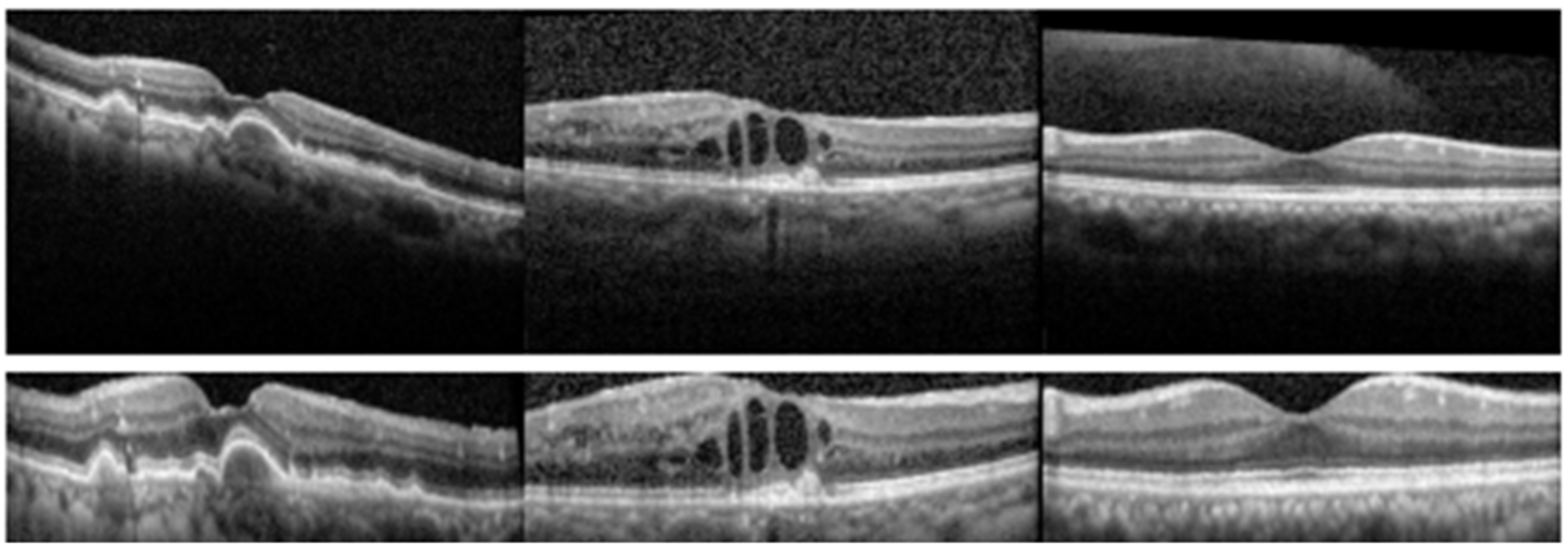
The small-scale retinal OCT dataset is obtained from clinics in Beijing hospital, using CIRRUS TM (Heidelberg Engineering Inc., Heidelberg, Germany). This dataset consists of 560 AMD, 560 DME and 560 normal (NOR) images. All the SD-OCT images are read and assessed by the trained graders. We first preprocessed these images using the preprocessing method in [14] which is mainly divided into three stages. (1) In the perceiving stage, the method detects the overall morphology of a retina. Firstly, the sparsity-based block matching and 3-D-filtering (BM3D) denosing method [34] is used to reduce noises of the OCT image, then the binarization, median filtering, morphological closing and morphological opening methods are used to obtain the subject of the image. (2) In the fitting stage, the method automatically chooses the set of data points and a fitting method (linear fitting or second-order polynomial fitting). (3) In the normalizing stage, the method normalizes the retinas by aligning them to a relatively unified morphology and crops the images to trim out insignificant space. Some examples are shown in Figure 5.

Then the preprocessed dataset is divided into training set of 840 images (280 AMD, 280 DME and 280 NOR) and test set of 840 images (280 AMD, 280 DME and 280 NOR). We finetuned all the layers of the sub-networks using the same batch size, Adam optimizer and input size as in large-scale experiment. The only difference is that we trained for 30 epochs in the small-scale dataset instead of 20. Each experiment conducts 10 times. The mean ± standard deviation of the value of accuracy, sensitivity and specificity were calculated.

We compared our algorithm with some state-of-the-art work. The algorithm of spatial pyramid matching using sparse coding (ScSPM) [14] utilizes techniques such as SIFT, SC, K-SVD, multi-scale max pooling and linear SVM. The algorithm of deep learning-based CNN (DL-based CNN) [35] removes the last several layers from the pre-trained Inception-v3 and regards the remaining part as a fixed feature extractor. Then the features are used as input of a CNN designed to learn the feature space shifts. Results in

Table 5. The performance (%) of the sub-networks on the clinical dataset.

		Accuracy	Sensitivity	Specificity
ScSPM [14]		97.75	96.67	98.30
DL-based CNN [35]		98.86	98.30	99.15
IBDL [9]		94.57	92.03	95.85
Sub-networks of Inception-v3	Mixed6	99.67 ± 0.08	99.50 ± 0.12	99.75 ± 0.06
	Mixed7	99.51 ± 0.17	99.26 ± 0.25	99.63 ± 0.13
	Mixed8	99.58 ± 0.13	99.37 ± 0.19	99.68 ± 0.10
	Mixed9	99.56 ± 0.17	99.35 ± 0.25	99.67 ± 0.13
	Mixed10	99.27 ± 0.41	98.90 ± 0.61	99.45 ± 0.31
Sub-networks of ResNet50	Ac37	99.49 ± 0.18	99.24 ± 0.26	99.62 ± 0.13
	Ac40	99.35 ± 0.19	99.02 ± 0.28	99.51 ± 0.14
	Ac43	99.34 ± 0.19	99.01 ± 0.29	99.50 ± 0.14
	Ac46	99.27 ± 0.19	98.90 ± 0.28	99.45 ± 0.14
	Ac49	99.09 ± 0.25	98.64 ± 0.38	99.32 ± 0.19
Sub-networks of DenseNet121	C5_b2	99.53 ± 0.16	99.30 ± 0.24	99.65 ± 0.12
	C5_b4	99.56 ± 0.17	99.35 ± 0.26	99.67 ± 0.13
	C5_b6	99.60 ± 0.18	99.40 ± 0.26	99.70 ± 0.13
	C5_b8	99.53 ± 0.18	99.30 ± 0.27	99.65 ± 0.13
	C5_b10	99.46 ± 0.23	99.19 ± 0.34	99.59 ± 0.17
	C5_b12	99.48 ± 0.17	99.23 ± 0.26	99.61 ± 0.13
	C5_b14	99.55 ± 0.16	99.33 ± 0.24	99.67 ± 0.12
	C5_b16	99.58 ± 0.11	99.37 ± 0.17	99.68 ± 0.08

show that all the sub-networks of Inception-v3, ResNet50 and DenseNet121 outperform ScSPM [14], DL-based CNN [35] and IBDL [9].

In the case of Inception-v3, “mixed6” reaches the highest accuracy of 99.67% and the minimal standard deviation of 0.08%. Note that method of finetuning complete inception-v3 (“mixed10”) only achieves accuracy of 99.21% and standard deviation of 0.41%. It shows improvement both in accuracy and stability of the sub-network removing deep layers, which means that the removal of deep convolution layer with a high-level feature in pre-trained Inception-v3 enhances the process of transfer learning.

Results of ResNet50 demonstrate similar conclusion. “Ac37” (99.49 ± 0.08%) outperforms all ResNet50 sub-networks discussed in the article, including complete ResNet50 (“mixed10” with 99.09 ± 0.25%).

Let us claim that “mixed6” and “Ac37” perform better than their corresponding entire network. In inferential statistics, the null hypothesis is that the mean accuracy of sub-network is the same as that of entire network. We measure the accuracy of ten repeated experiments and conduct one-way analysis of variance with α = 0.05. As

Table 6. One-way analysis of variance (ANOVA) with α = 0.05.

	Average	Standard Deviation	F	p-Value	F Crit
Mixed6	99.67	0.08	8.984	7.73 × 10−3	4.414
Mixed10	99.27	0.41
Ac37	99.49	0.18	16.690	6.94 × 10−4	4.414
Ac49	99.09	0.25

shows, P-value is 7.73 × 10⁻³ in the Inception-v3 group and 6.94 × 10⁻⁴ in the ResNet group, both far less than α; F value is 8.984 in the Inception-v3 group and 16.690 in the ResNet group, both greater than the critical value 4.414. Results mean that we reject the null hypothesis. The analysis demonstrates significant difference of accuracy between the sub-network and entire network.

Compared with Inception-v3 and ResNet50, the improvement of diagnostic performance is limited in the case of DenseNet. Accuracy of the best sub-network of DenseNet121 (“C5_b6”) is only 0.02% higher than that of complete DenseNet121 (“C5_b16”), with 0.07% decline in standard deviation. It can be well explained in terms of architecture different from Inception-v3 and ResNet50, as deep layers of DenseNet121 receive concatenation of all the preceding feature maps, which reserve information of shallow layers in the output. Thus, the removal of the deep layer has little influence on the classification. However, similar performance is obtained with only 78% of trainable parameters, and “C5_b6” still beats other sub-networks in DenseNet121.

Overall, the removal of deep layers in Inception-v3 and ResNet50 improves the accuracy and stability significantly on the small-scale dataset. Due to the dense connection structure of DenseNet121, a similar improvement does not exist in this case. The best sub-network among them is “Mixed6” with accuracy of 99.67% and standard deviation of 0.08%. The number of trainable parameters of “Mixed6” is also acceptable compared to other sub-networks.

4. Conclusions

Traditionally, pre-trained networks such as Inception-v3, ResNet, DenseNet are transferred into medical image applications as a whole. This paper proposes a strategy to obtain their 5–8 sub-networks by removing some deep layers, finetunes, and tests their performance for identification of macular diseases from optical coherence tomography images on two different scale OCT datasets. Optimized deep convolutional neural networks are obtained, i.e. Inception-v3 removing the last 4 blocks, ResNet50 removing the last 3 or 4 blocks, and DenseNet121 removing the last 10 or 12 basic blocks in the last dense block, which could improve diagnostic performance and computational efficiency compared to Inception-v3, ResNet50 and DenseNet121, respectively, in the process of transfer learning on OCT data.