Numerical Modeling of Wave Disturbances in the Process of Ship Movement Control

School of Computer Science at the Faculty of Navigation, Maritime University of Szczecin, Wały Chrobrego 1, Szczecin 70500, Poland
Algorithms 2018, 11(9), 130; https://doi.org/10.3390/a11090130
Submission received: 19 July 2018
/
Revised: 13 August 2018
/
Accepted: 29 August 2018
/
Published: 31 August 2018
(This article belongs to the Special Issue Modeling Computing and Data Handling for Marine Transportation)
Abstract
:The article presents a numerical model of sea wave generation as an implementation of the stochastic process with a spectrum of wave angular velocity. Based on the wave spectrum, a forming filter is determined, and its input is fed with white noise. The resulting signal added to the angular speed of a ship represents disturbances acting on the ship’s hull as a result of wave impact. The model was used for simulation tests of the influence of disturbances on the course stabilization system of the ship.
1. Introduction
A typical practice in designing an automatic control system is to build a mathematical model of an object (or process), and on this basis to make a synthesis of a control system (controller, algorithm). Then, before implementation, the created control algorithm is tested (if possible) by computer simulation and tuned in right after installation. Simulation is therefore the first step in checking the stability of the system and algorithm operation, so it should reflect reality as faithfully as possible, accounting for disturbances.
The process of ship movement control is characterized by a high level of external disturbances. Due to the manner of their influence, disturbances can be divided into two groups. Disturbances of one type affect ship dynamics (changes in water depth or loading condition, etc.); the other type is additive disturbances, whose effects are observed as additional signals superimposed on a ship’s heading, angular speed, drift angle, etc. The latter group also includes disturbances from currents, winds, and waves. Although they are correlated, these disturbances are usually divided into three different types of signals. This article focuses on disturbances from wind-generated waves, as they are the most essential from the viewpoint of the automatic ship movement control problem.
Literature on the subject abounds, with publications presenting complex models of sea waves related to specific water areas [1,2]. Other articles covering the topic under consideration address wave filters [3,4,5,6,7,8], as a standard based on the Kalman filter. Similar topics are also discussed in other works [9,10,11,12,13].
The article presents a numerical model of sea wave generation as a method alternative to the existing ones. The presented solution can be universally used in simulations of automatic ship movement control systems, tackling various problems. This is often difficult in the case of solutions presented in the literature on the subject. This restriction often results from the complexity of the models and the assumptions made. The proposed model is easy to implement and still takes into account all relevant components. The model was verified in simulations testing the influence of disturbances on the operation of the ship course stabilization system.
2. Wave Disturbances Generated by Wind
Surface layers of water in the sea and the air above are rarely calm. Statistical data on weather conditions prevailing in the North Atlantic show that, on average, the weather is windless only for about seven days a year [14]. In the remaining period, winds blow with different forces and from different directions, and the sea is more or less wavy. Wind-induced waves are formed by the impact of wind on the water; that is, kinetic energy from the atmosphere is transferred to the surface of the sea, creating free deformations. The size of the waves depends on the speed of wind-generating waves (the stronger the wind is, the larger wave dimensions can be), the duration of the wind blowing above the water from the same direction (in practice 15°), and the distance of fetch. Waves that appear on the surface of the seas and oceans make up an irregular interfered signal composed of a series of monochromatic waves. A set of interfered waves contains a whole spectrum of waves with different lengths, periods, speeds, and heights, so disturbances from waves can be regarded as an implementation of a stochastic process involving a specific spectrum. An example of such a description appointed by research based on real measurements is the spectrum in this form [14]:
where
The above values are associated with wave parameters (height , length) and depend on the sea state, as shown in Table 1. This table also approximately indicates the relation between wind speed (Beaufort wind scale) and sea state (Douglas scale).
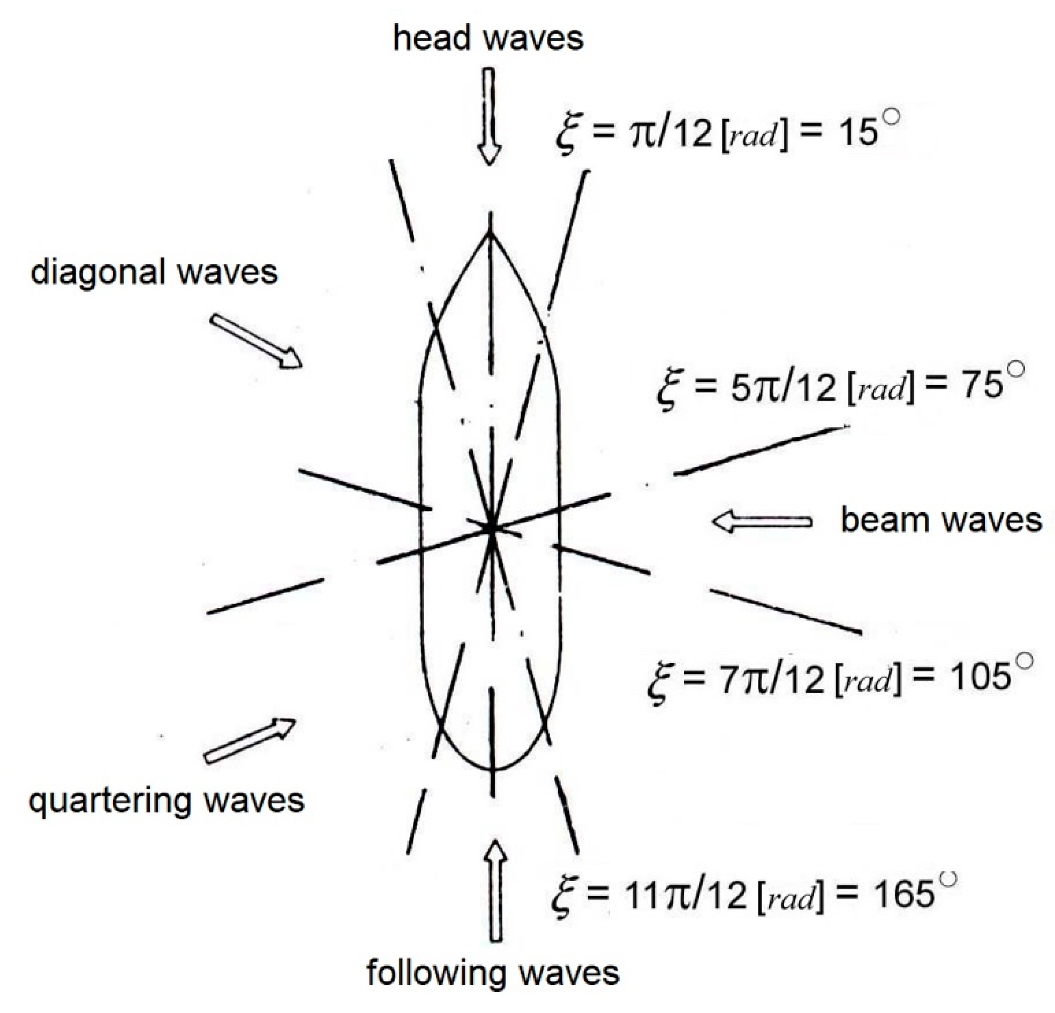
In the automatic course control system, the value of deviation from a preset course depends on wave energy, as well as a ship’s speed and wave angle (Figure 2). In this approach, we can consider the following situations:
- Waves coming at a specific angle from the direction opposite to ship movement (diagonal waves);
- waves coming at an angle, but in the direction of ship movement (quartering waves);
- waves coming from the bow (head waves);
- waves perpendicular to the ship side (beam waves);
- waves striking the stern (following waves).
The greatest changes in the heading angle of the ship at low speeds occur in case of transverse waves, whereas the smallest impact comes from diagonal and quartering waves; in case of diagonal and head waves, heading deviations (yawing) get larger as the ship speed increases. Taking into account the ship speed and wave angle, we can transform spectrum (1) to this form (determined by research based on real measurements) [14]:
where
- —parameter dependent on parameter ;
- —parameter calculated from the formula ;
- V—ship’s speed;
- G—gravitational acceleration;
- —wave angle (Figure 2).
The effect of wave action on the process of ship movement control (in various control problems) can easily be determined by measuring a ship’s angular velocity. The signal of angular speed is a sum of two components: One formed due to rudder deflection, and the other due to waves. The spectrum of angular velocity is created by transforming the spectrum of wave ordinates (2) and takes this form (appointed by research based on real measurements) [14]:
where
- —spectral density of wave angular velocity;
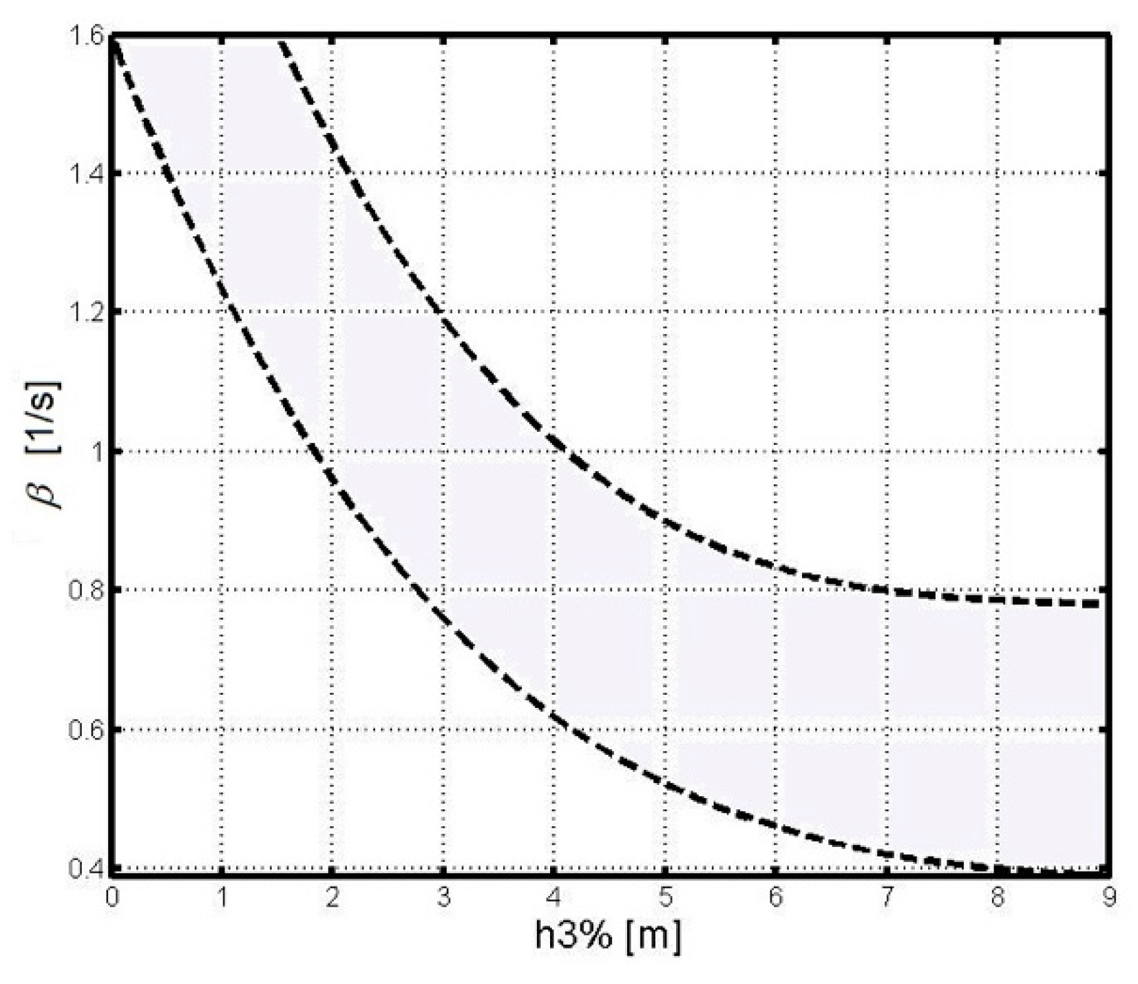
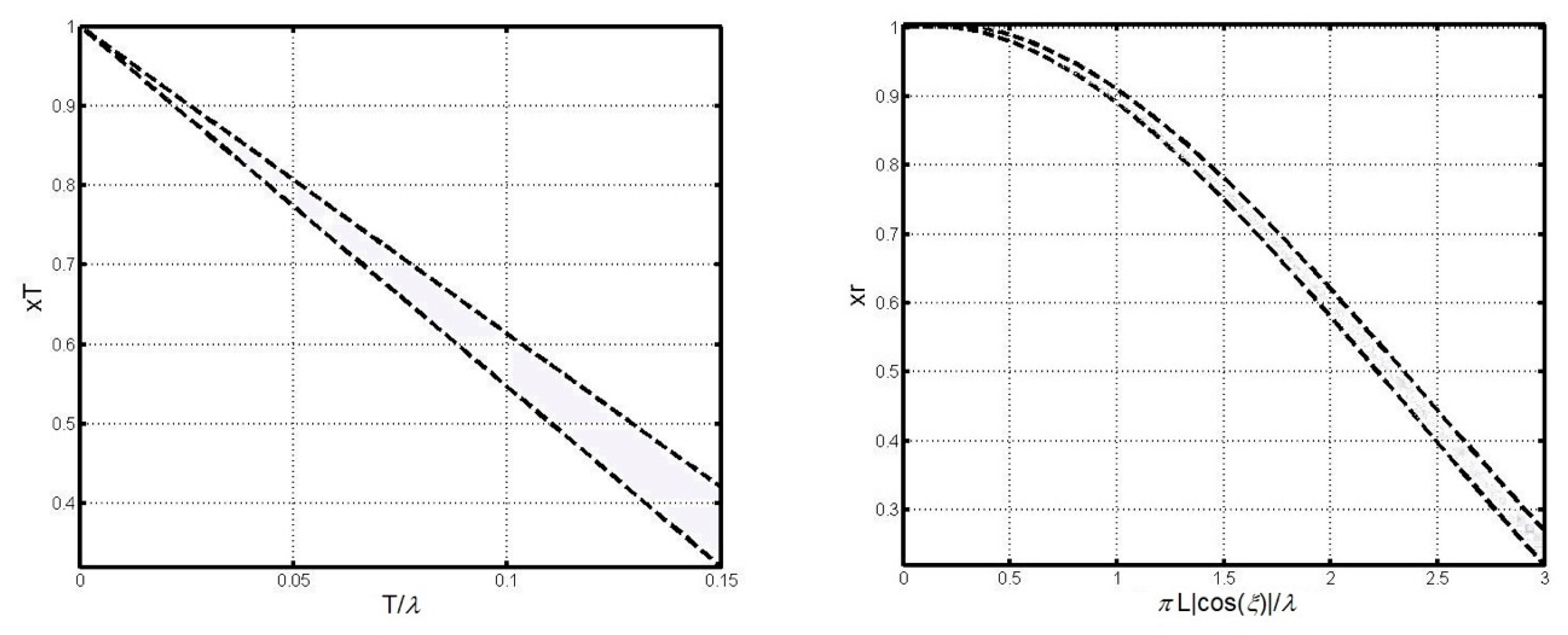
- —dimensionless reducing parameters (Figure 3) dependent on the length of the ship (L), wavelength (), and the ship’s maximum draught marked by the waterplane (T).
It should be noted that spectral density (3), due to the expression in the numerator , faithfully represents the power of the wave signal for angles differing from 90° by at least 15° (for diagonal, quartering, head, and following waves).
In order to use the spectrum of wave angular velocity (3) acting as disturbances affecting the ship hull due to waves, the forming filter:
should be used to pass white noise through it (stochastic process with zero expected value and steady spectral density); then, the formed signal rw should be added to—or, for positive wave angles, subtracted from—the ship’s angular speed caused by rudder deflection.
Filter (4) is obtained from this relation:
Using Lagrange interpolation (Algorithm 1), where average values of parameters are adopted in the nodes , we get:
where
- —a function returning the value of the polynomial with coefficients written in a table p, in a set point xi;
- —function returning the value for , value for and value for .
| Algorithm 1 Using Lagrange interpolation |
| % x = [x0, x1, …, xN], y = [y0, y1, …, yN] |
| % p—coefficients of Lagrange polynomial |
| function p = lagranp(x,y) |
| N = length(x) − 1; |
| p = 0; |
| for m = 1:N + 1 |
| P = 1; |
| for k = 1:N + 1 |
| if k ~= m |
| P = conv(P,[1 − x(k)])/(x(m) − x(k)); |
| End |
| End |
| p = p + y(m) * P; |
| end |
| end |
In relation to Equation (6), input parameters of the numerical model of sea wave generation acting on the ship hull are:
- Parameters associated with the wave:
- -
- Wave angle ;
- -
- wave height ;
- -
- wave length ;
- parameters of the ship:
- -
- Maximum draft T;
- -
- length L;
- -
- speed V.
In addition, taking into account the data from Table 1, we can refer to the model input to wind force (Beaufort wind scale) or to sea state (Douglas scale).
3. Computing Experiments
The experiments have been made in a MATLAB/Simulink environment. A de Witt-Oppe model [15] represented a real ship, incorporating the dynamics of the steering gear [16]:
where
- —Cartesian coordinates (ship’s position);
- —deviation from the course;
- —angular velocity;
- —longitudinal speed;
- —transverse speed;
- —rudder angle;
- —rudder angle setting;
- —maximum rudder deflection;
- —maximum rate of turn of the rudder;
- St—propeller thrust;
- —coefficients determined from model tests (different for different types of vessels).
The ship movement parameters adopted herein are those of a ship of mariner class, motor ship (m.s.). Compass Island [15]: [1/s], [s/rad2], [1/s2], [1/s], [m/rad2], [m/s2], [m/rad], [m/s2/rad3]. This particular ship has the following characteristics: 9214 gross registered tons [t], 13,498 DWT, single screw, length L = 172 [m], maximum draft indicated by the waterplane T = 8 [m], maximum speed 20 [w], maximum (minimum) angular velocity [rad/s] ( [rad/s]), maximum (minimum) rudder angle [rad] ( [rad]), maximum (minimum) rudder rate of turn [rad/s] ([rad/s]).
The established initial parameters of the simulation were as follow: Angular velocity , deviation from the course , rudder angle , ship’s speed .
A linear quadratic regulator (LQR) was chosen as the control algorithm of the ship course stabilization system. The LQR regulator was synthesized using a Nomoto model [16]:
The quality control criterion was this functional:
where
—a coefficient greater than zero, which is interpreted as a compromise between the deviation from the course (angle of yaw) and the rudder angle (steering gear load), arbitrarily adopted here as 1.
Then, the control for LQR can be expressed by this formula:
where , .
Without compromising the generality of the research, it was assumed that parameters , , do not change their value during computational experiments.
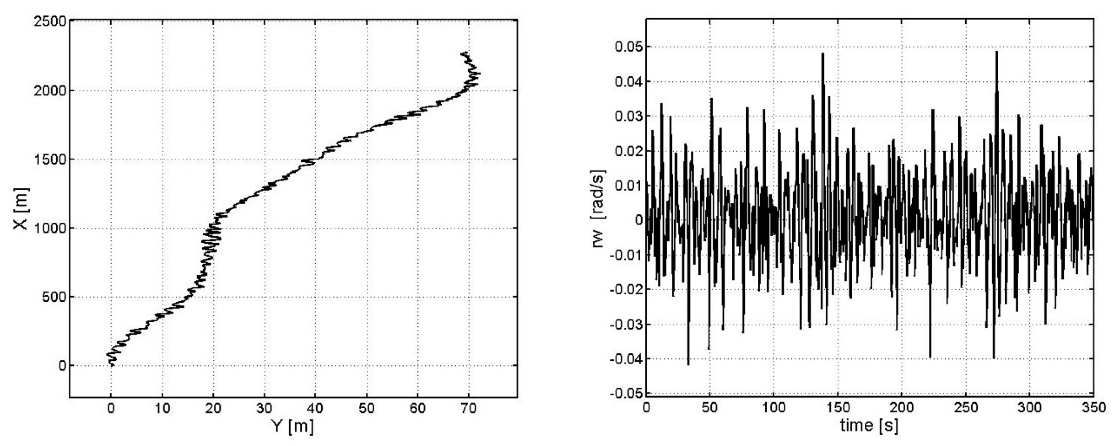
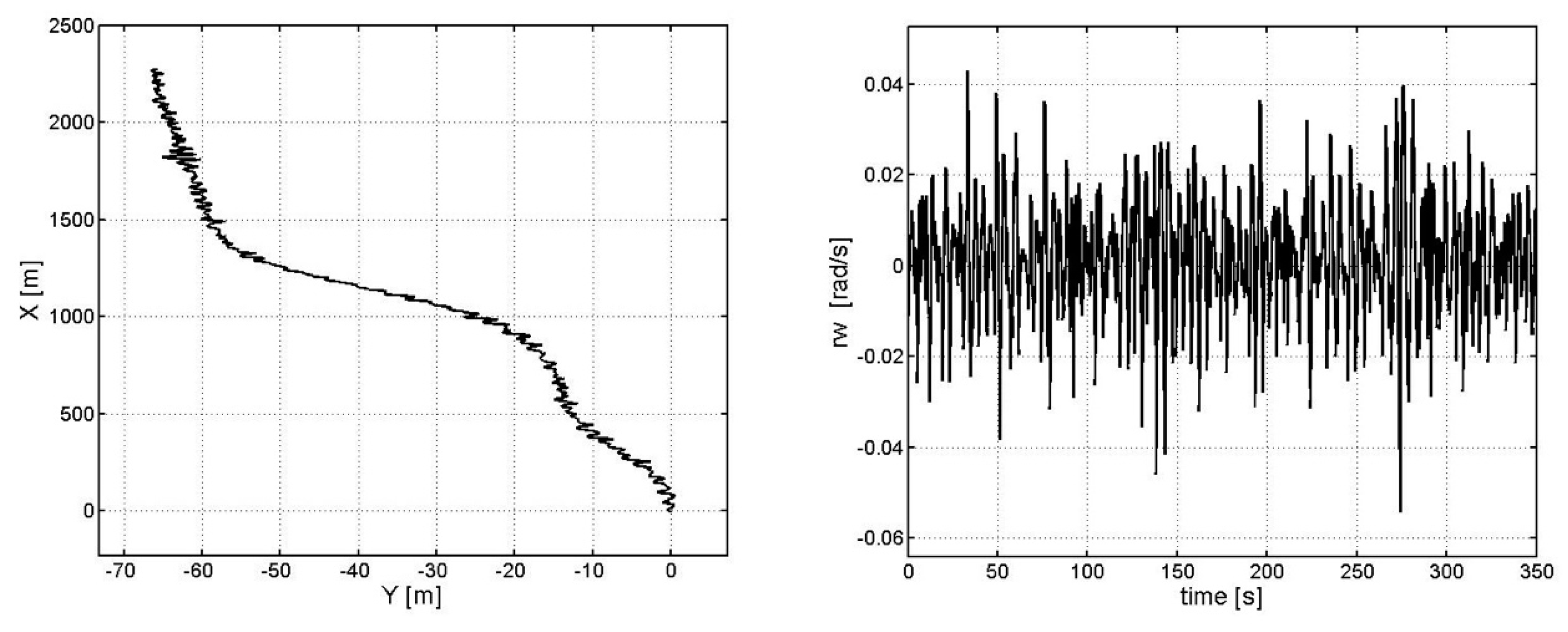
The computing experiments were intended to investigate the operational correctness of numerical-model-generating waves acting on the ship hull. Figure 4, Figure 5, Figure 6 and Figure 7 show ship movement trajectories (course setting was 0°) for disturbances from four types of wave. The first trajectory was obtained at sea state 4 and for the wave angle (diagonal waves); the second trajectory was produced at sea state 5 and for the wave angle (diagonal waves); the third one was also obtained at sea state 5 , but for the wave angle (head waves), whereas the fourth was obtained at sea state 6 and for the wave angle (diagonal waves). In all four situations, the quality control is high (note the scale used due to the specificity of particular cases), although in the second case the ship is much more pushed to the left (port side, because ) than in the first case (to the right—starboard, because ), due to higher sea state. In the third case, despite sea state 5, the ship is drifting less than in the second situation, due to the zero angle of the head waves. In the fourth case, the ship has the strongest drift (to the right—starboard, because ), due to the highest sea state 6. This happens even if the wave angle in absolute terms is the smallest of all presented situations involving diagonal waves.
In addition, Figure 4, Figure 5, Figure 6 and Figure 7 illustrate disturbance signals added to the ship’s angular velocity caused by rudder deflection. One can observe that, as expected, the absolute value of the signal increases with increasing sea state, whereas for the steady sea state it decreases for smaller absolute wave angles.
The presented situations are typical of the research done. In all examined cases, the model correctly executed hull-affecting disturbances that corresponded to sea waves induced by wind.
4. Conclusions
The article presents a numerical model of sea wave generation, which was positively tested in a ship course stabilization problem. The stabilization control algorithm was provided by an LQR regulator.
Wave generation is required for ship movement simulations designed for various problems (navigation along a preset trajectory, dynamic positioning systems, collision avoidance, etc.) [17,18,19,20], and makes up a preliminary stage in designing control systems before sea trials of a ship. The inclusion of wave disturbance is also recommended in other problems relating to modern marine navigation [21,22,23,24,25,26,27,28,29].
The author plans to apply stochastic disturbance of a ship’s angular speed in developing original systems of ship movement control.
Funding
This research outcome has been achieved under the grant No 1/S/ITM/16 financed from a subsidy of the Ministry of Science and Higher Education in Poland for statutory activities.
Conflicts of Interest
The author declares no conflict of interest.
References
- Nitta, T.; Nanbu, M.; Yoshizaki, M. Wave disturbances over the China continent and the Eastern China Sea in February 1968. J. Meteorol. Soc. Jpn. 1973, 51, 11–28. [Google Scholar] [CrossRef]
- Sarker, M. Numerical modelling of waves and surge from Cyclone Chapala (2015) in the Arabian Sea. Ocean Eng. 2018, 158, 299–310. [Google Scholar] [CrossRef]
- Fossen, T.I. High performance ship autopilot with wave filter. In Proceedings of the 10th International Ship Control Systems Symposium, Ottawa, ON, Canada, 25–29 October 1993; pp. 2271–2285. [Google Scholar]
- Holzhuter, T. On the robustness of course keeping autopilots. In Proceedings of the IFAC Workshop on Control Applications n Marine Systems, Hamburg, Italy, 8–10 April 1992; pp. 235–244. [Google Scholar]
- Holzhuter, T.; Strauch, H. A commercial adaptive autopilot for ships: Design and experimental experience. In Proceedings of the 10th IFAC World Congress, Munich, Germany, 27–31 July 1987; pp. 226–230. [Google Scholar]
- Lauvdal, T.; Fossen, T.I. A globally stable adaptive ship autopilot with wave filter using only yaw angle measurements. In Proceedings of the 3rd IFAC Workshop on Control Applications in Marine Systems, Trondheim, Norway, 10–12 May 1995; pp. 262–269. [Google Scholar]
- Saelid, S.; Janssen, N.A. Adaptive Ship Autopilot with Wave Filter. MIC 1983, 4, 33–46. [Google Scholar] [CrossRef]
- Wang, X.; Xu, H. Robust autopilot with wave filter for ship steering. JMSA 2006, 5, 24–29. [Google Scholar]
- David, C.G.; Roeber, V.; Goseberg, N.; Schlurmann, T. Generation and propagation of ship-borne waves—Solutions from a Boussinesq-type model. Coast. Eng. 2017, 127, 170–187. [Google Scholar] [CrossRef]
- Li, W.; Du, J.; Sun, Y.; Song, J. Modeling and simulation of wave disturbances for dynamic positioning ship. J. Dalian Marit. Univ. 2013, 1, 6–10. [Google Scholar]
- Liceaga-Castro, E.; Molen, G.M. Submarine H/sup /spl infin// depth control under wave disturbances. IEEE Trans. Control Syst. Technol. 1995, 3, 338–346. [Google Scholar] [CrossRef]
- Sandaruwan, D.; Kodikara, N.; Rosa, R.; Keppitiyagoma, C. Modeling and Simulation of Environmental Disturbances for Six degrees of Freedom Ocean Surface Vehicle. Sri Lankan J. Phys. 2009, 10, 39–57. [Google Scholar] [CrossRef]
- Wenhua, L.; Jialu, D.; Yuqing, S.; Haiquan, C.; Yindong, Z.; Jian, S. Modeling and simulation of marine environmental disturbances for dynamic positioned ship. In Proceedings of the 31st Chinese Control Conference, Hefei, China, 25–27 July 2012; pp. 1938–1943. [Google Scholar]
- Lerner, D.M. Control of Marine Moving Objects; Sudostroenie: Leningrad, Russia, 1979. [Google Scholar]
- Wit, C.; Oppe, J. Optimal collision avoidance in unconfined waters. J. Inst. Navig. 1984, 26, 296–303. [Google Scholar] [CrossRef]
- Fossen, T.I. Guidance and Control of Ocean Vehicles; John Wiley & Sons: Chichester, UK, 1994. [Google Scholar]
- Borkowski, P. Adaptive ship course-keeping system. Arch. Transp. Syst. Telemat. 2014, 7, 19–23. [Google Scholar]
- Omerdic, E.; Roberts, G.; Vukic, Z. A fuzzy track-keeping autopilot for ship steering. J. Mar. Eng. Technol. 2003, 2, 23–35. [Google Scholar]
- Perera, L.P.; Soares, C.G. Pre-filtered Sliding Mode Control for Nonlinear Ship Steering Associated with Disturbances. Ocean Eng. 2012, 51, 49–62. [Google Scholar] [CrossRef]
- Ren, J.; Zhang, X. Ship course-keeping adaptive fuzzy controller design using command filtering with minimal parametrization. In Proceedings of the 25th Chinese Control and Decision Conference (CCDC), Guiyang, China, 25–27 May 2013; pp. 243–247. [Google Scholar]
- Borkowski, P. Algorithm of multi-sensor navigational data fusion—Testing of estimation quality. Pol. J. Environ. Stud. 2008, 17, 43–47. [Google Scholar]
- Borkowski, P. The ship movement trajectory prediction algorithm using navigational data fusion. Sensors 2017, 17, 1432. [Google Scholar] [CrossRef] [PubMed]
- Guze, S.; Smolarek, L.; Weintrit, A. The area-dynamic approach to the assessment of the risks of ship collision in the restricted water. Sci. J. Marit. Univ. Szczec. 2016, 117, 88–93. [Google Scholar]
- Kazimierski, W. Proposal of neural approach to maritime radar and automatic identification system tracks association. IET Radar Sonar Navig. 2017, 11, 729–735. [Google Scholar] [CrossRef]
- Kazimierski, W.; Stateczny, A. Radar and Automatic Identification System Track Fusion in an Electronic Chart Display and Information System. J. Navig. 2015, 68, 1141–1154. [Google Scholar] [CrossRef]
- Kijewska, M. A graphical model to determine the influence of surface currents on small objects immersed in water. Sci. J. Mar. Univ. Szczec. 2016, 47, 170–175. [Google Scholar]
- Ochin, E.; Dobryakova, L.; Pietrzykowski, Z.; Borkowski, P. The application of cryptography and steganography in the integration of seaport security subsystems. Sci. J. Marit. Univ. Szczec. 2011, 26, 80–87. [Google Scholar]
- Wawrzyniak, N.; Stateczny, A. MSIS image postioning in port areas with the aid of comparative navigation methods. Pol. Marit. Res. 2017, 24, 32–41. [Google Scholar] [CrossRef]
- Zaniewicz, G.; Kazimierski, W.; Bodus-Olkowska, I. Integration of Spatial Data from External Sensors in the Mobile Navigation System for Inland Shipping. In Proceedings of the Baltic Geodetic Congress, Gdansk, Poland, 2–4 June 2016; pp. 165–170. [Google Scholar]
Figure 1.
Boundary relation between the parameter beta and wave height.

Figure 2.
Definition of the wave angle.

Figure 3.
Boundary dependences of reducing parameters.

Figure 4.
The trajectory of ship movement and signal of angular speed disturbance rw for sea state 4 and the wave angle −π/4.
Figure 4.
The trajectory of ship movement and signal of angular speed disturbance rw for sea state 4 and the wave angle −π/4.
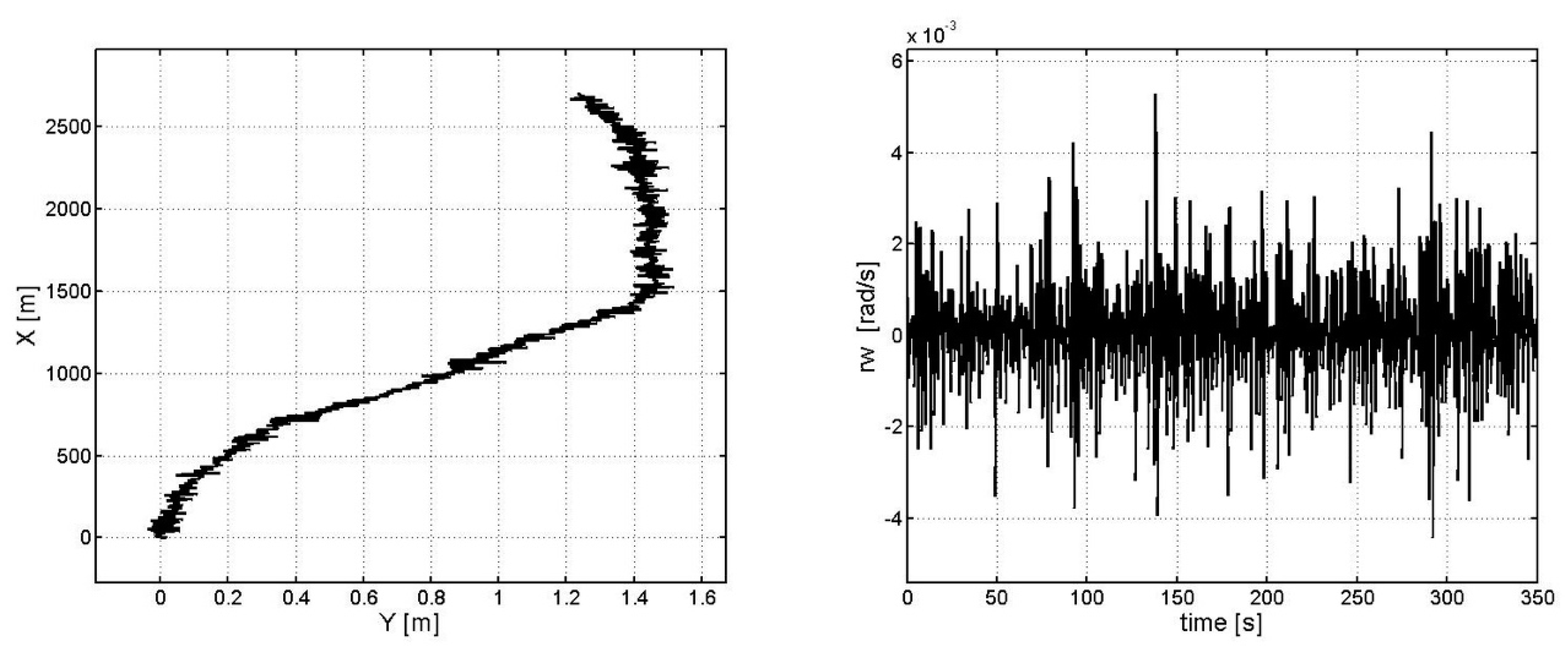
Figure 5.
The trajectory of ship movement and signal of angular speed disturbance rw for sea state 5 and the wave angle 5π/12.
Figure 5.
The trajectory of ship movement and signal of angular speed disturbance rw for sea state 5 and the wave angle 5π/12.

Figure 6.
The trajectory of ship movement and signal of angular speed disturbance rw for sea state 5 and the wave angle 0.
Figure 6.
The trajectory of ship movement and signal of angular speed disturbance rw for sea state 5 and the wave angle 0.
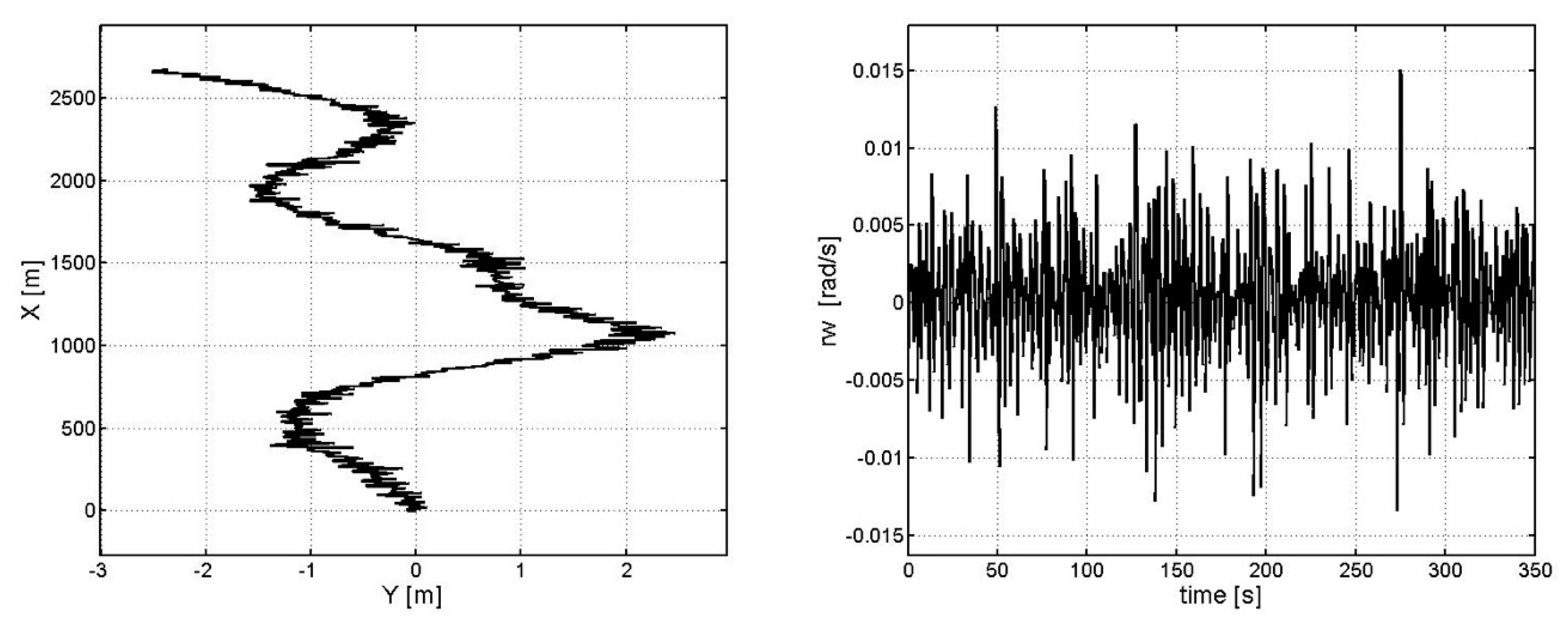
Figure 7.
The trajectory of ship movement and signal of angular speed disturbance rw for sea state 6 and the wave angle −π/5.
Figure 7.
The trajectory of ship movement and signal of angular speed disturbance rw for sea state 6 and the wave angle −π/5.

Table 1.
Summary of selected parameters of waves depending on the sea state and the Beaufort wind scale.
Table 1.
Summary of selected parameters of waves depending on the sea state and the Beaufort wind scale.
| Sea State | Sea State Designation | Probability of Occurrence [%] | Maximum Wave Length [m] | Beaufort Wind Scale (Approx.) | |
|---|---|---|---|---|---|
| 0 | calm–glassy | 11.2486 | 0 | – | 0 |
| 1 | calm–rippled | 0.00–0.25 | 5 | 1 | |
| 2 | smooth wavelets | 0.25–0.75 | 25 | 2–3 | |
| 3 | slight | 31.6851 | 0.75–1.25 | 50 | 4 |
| 4 | moderate | 40.1944 | 1.25–2.00 | 75 | 5 |
| 5 | rough | 12.8005 | 2.00–3.50 | 100 | 6 |
| 6 | very rough | 3.0253 | 3.50–6.00 | 135 | 7 |
| 7 | high | 0.9263 | 6.00–8.50 | 200 | 8 |
| 8 | very high | 0.1190 | 8.50–11.0 | 250 | 9–10 |
| 9 | phenomenal | 0.0009 | 11.0–… | >250 | 11–12 |
© 2018 by the author. Licensee MDPI, Basel, Switzerland. This article is an open access article distributed under the terms and conditions of the Creative Commons Attribution (CC BY) license (http://creativecommons.org/licenses/by/4.0/).
Share and Cite
MDPI and ACS Style
Borkowski, P. Numerical Modeling of Wave Disturbances in the Process of Ship Movement Control. Algorithms 2018, 11, 130. https://doi.org/10.3390/a11090130
AMA Style
Borkowski P. Numerical Modeling of Wave Disturbances in the Process of Ship Movement Control. Algorithms. 2018; 11(9):130. https://doi.org/10.3390/a11090130
Chicago/Turabian StyleBorkowski, Piotr. 2018. "Numerical Modeling of Wave Disturbances in the Process of Ship Movement Control" Algorithms 11, no. 9: 130. https://doi.org/10.3390/a11090130
Note that from the first issue of 2016, this journal uses article numbers instead of page numbers. See further details here.