A Forecast Model of the Number of Containers for Containership Voyage

Abstract

Container ships must pass through multiple ports of call during a voyage. Therefore, forecasting container volume information at the port of origin followed by sending such information to subsequent ports is crucial for container terminal management and container stowage personnel. Numerous factors influence container allocation to container ships for a voyage, and the degree of influence varies, engendering a complex nonlinearity. Therefore, this paper proposes a model based on gray relational analysis (GRA) and mixed kernel support vector machine (SVM) for predicting container allocation to a container ship for a voyage. First, in this model, the weights of influencing factors are determined through GRA. Then, the weighted factors serve as the input of the SVM model, and SVM model parameters are optimized through a genetic algorithm. Numerical simulations revealed that the proposed model could effectively predict the number of containers for container ship voyage and that it exhibited strong generalization ability and high accuracy. Accordingly, this model provides a new method for predicting container volume for a voyage.

1. Introduction

Container transportation is a highly complicated process and involves numerous parties, necessitating close cooperation between ports, ships, shipping companies, and other relevant departments. Therefore, container transportation management is characterized by extremely detailed planning [1,2]. For example, container terminals must formulate strategies such as berthing plans [3], container truck dispatch plans, yard planning systems, and yard stowage plans [4,5,6]. In addition, ships or shipping companies must formulate voyage stowage plans for container ships at the port of departure. The number of containers in the subsequent port must be predicted, and such prediction information forms a crucial basis for the subsequent plan. These processes must be completed before the development of a stowage system for full-route container ships [7].

Changes in the number of containers allocated to container ships are influenced by several factors, which are characterized by uncertain information; this thus engenders a complex nonlinear relationship between the number of allocated containers and influencing factors [8]. The number of allocated containers is influenced by the port of call, local GDP, port industrial structures, and collection and distribution systems; by shipping company-related factors such as the capacity of a company, inland turnaround time of containers, seasonal changes in cargo volume, and quantity of containers managed by the company; and by ship-related factors such as the transportation capacity of a single ship and the full-container-loading rate of the ship. Each of these factors exerts distinct effects on the number of containers allocated to a container ship for one voyage; therefore, describing these factors by using an accurate mathematical model is difficult [9]. Traditional methods such as time series forecasting (including exponential smoothing [10], gray prediction [11], moving average [12], and seasonal periodic variation [13] approaches) and regression forecasting [14] typically rely on certain mathematical theories and assumptions and necessitate the establishment of mathematical models through deductive reasoning without considering influencing factors. By contrast, neural networks—constituting a nonlinear and nonparametric model—can describe the nonlinear relationship between a premeasured quantity and influencing factors, and they have self-learning and self-adaptation abilities to effectively avoid prediction errors caused by assumptions; accordingly, neural networks have been extensively applied in various project prediction processes. However, neural networks [15] have drawbacks such as an indeterminable network structure, overfitting, local minimum, and “curse of dimensionality”. Support vector machines (SVMs) [16] solve the aforementioned drawbacks of neural networks by minimizing structural risk, and SVMs are highly suitable for predicting the number of containers allocated to a container ship for one voyage, a problem that involves characteristics such as nonlinearity, high dimensionality, and a small-scale sample [17,18,19,20]. An SVM entails the selection of a kernel function, thus demonstrating the nonlinear processing ability of the learning machine; because a kernel function is selected [21], a feature space is defined [22,23]. Nevertheless, a single kernel function cannot afford learning ability and generalization ability simultaneously in an SVM [24]. This paper proposes mixed kernels, which can effectively improve the predictive performance of an SVM model with weighted arrays of polynomial and radial basis kernel functions.

As mentioned, each of the aforementioned factors exerts distinct effects on the various factors influencing the number of allocated containers in one voyage. If such differences are neglected, the prediction results would be distorted [25]. Therefore, this paper proposes a model based on gray relational analysis (GRA) theory [26] and mixed kernel SVM for predicting container allocation to a container ship. In this model, GRA is applied to obtain the gray relational ordinal of each influencing factor, thus determining the weight of each factor. Subsequently, the weighted influencing factors serve as inputs to the SVM model, thus resulting in the mixed kernel SVM prediction model. To solve more complex parameter optimization problem in the mixed kernel SVM model, a genetic algorithm (GA) is adopted for SVM parameter optimization [27,28]. Simulations are presented herein to demonstrate the effectiveness of this method. The novelty of this paper is that it proposes a mixed kernel SVM model for predicting the number of containers allocated to a container ship for a voyage.

2. Gray Relation Analysis

Gray relation analysis is the serialization and patterning of the gray relation between an operating mechanism and its physical prototype, which is either not clear at all or certainly lacks a physical prototype. The “essence” of the analysis is an overall comparison of the measurements with a reference system [29]. The technical connotation of gray relation analysis is: (i) acquiring information about the differences between sequences and establishing a difference information space; (ii) establishing and calculating the differences to compare with the measurements (gray correlation degree); and (iii) establishing the order of the relation among the factors to determine the weight of each influencing factor [30]. The calculation steps are as follows [31]:

Step 1: Set a sequence $X_0=\left(\begin{array}{cccccc}{x}_0\left(1\right),& x_0\left(2\right),& \cdots ,& x_0\left(k\right),& \cdots ,& x_0\left(n\right)\end{array}\right)$ as the reference sequence, i.e., the object of study and $X_i=\left(\begin{array}{cccccc}{x}_i\left(1\right),& x_i\left(2\right),& \cdots ,& x_i\left(k\right),& \cdots ,& x_i\left(n\right),\end{array}\right)\left(i=1,2,\cdots ,m\right)$ as the comparative sequence, i.e., the influencing factors.

Step 2: Data conversion or dimensionless processing for which, the initialization conversion is adopted in this study, wherein the first variable of each sequence is used to remove all the other variables to obtain the initial value of the image $Y_i\left(k\right)$:

$$Y_i\left(k\right)=\frac{X_i\left(k\right)}{X_i\left(1\right)}$$

(1)

where $i=0,1,2,\cdots ,m$ and $k=1,2,\cdots ,n$.

Step 3: Calculate the gray relation coefficient $\gamma \left(Y_0\left(k\right),Y_i\left(k\right)\right)$ of $Y_0\left(k\right)$ and $Y_i\left(k\right)$:

$$\gamma \left(Y_0\left(k\right),Y_i\left(k\right)\right)=\frac{\underset{i}{\min } \underset{k}{\min } {\Delta }_{0i} \left(k\right)+\zeta \underset{i}{\max } \underset{k}{\max } {\Delta }_{0i}\left(k\right)}{{\Delta }_{0i}\left(k\right)+\zeta \underset{i}{\max } \underset{k}{\max } {\Delta }_{0i}\left(k\right)}$$

(2)

$${\Delta }_{0i}\left(k\right)=\left|Y_0\left(k\right)-Y_i\left(k\right)\right|$$

(3)

where $\zeta \in \left[0,1\right]$ is the resolution coefficient. The resolution coefficient $\zeta$ determines the result of the correlation analysis. The literature [32] shows that when $\zeta \le 0.05$, the resolution of the correlation degree changes more obviously, so $\zeta =0.05$ is selected in this paper.

Step 4: Calculate the correlation degree $\gamma \left(Y_0,Y_i\right)$ of the subsequence $Y_i\left(k\right)$ of the parent sequence $Y_0\left(k\right)$:

$$\gamma \left(Y_0,Y_i\right)=\frac{1}{n}{\displaystyle \sum _{k=1}^n\gamma \left(Y_0\left(k\right),Y_i\left(k\right)\right)}$$

(4)

Compare $\gamma \left(Y_0,Y_i\right)$ with $\gamma \left(Y_0,Y_j\right)\left(i\ne j\right)$, and if $\gamma \left(Y_0,Y_i\right)>\gamma \left(Y_0,Y_j\right)$, it is indicated that the $i\mathrm{th}$ factor has a greater impact on the results than the $j\mathrm{th}$ factor.

Step 5: Calculate the weight of the various influencing factors:

$$w\left(Y_i\right)=\frac{\gamma \left(Y_0,Y_i\right)}{{\displaystyle \sum _{i=1}^m\gamma \left(Y_0,Y_i\right)}}$$

(5)

3. Mixed Kernel Function SVM Prediction Model

3.1. Support Vector Machine for Regression

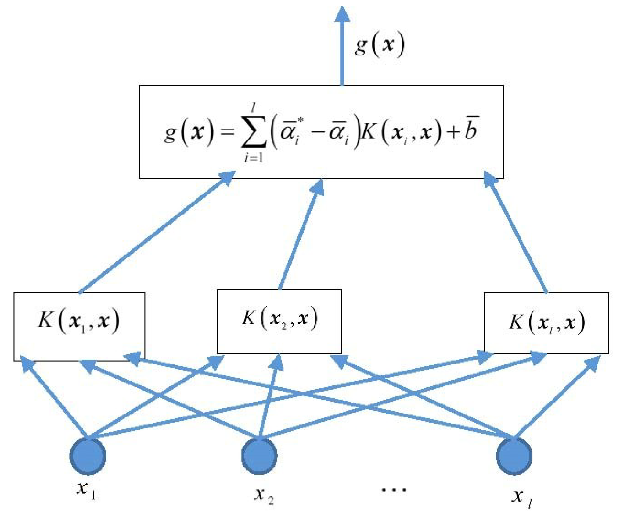
A support vector machine (SVM) was officially proposed by Cortes & Vapnik in 1995, which was a significant achievement in the field of machine learning. Vapnik et al. [16,17] introduced an insensitive loss function $\epsilon$ based on the SVM classification and obtained a support vector machine for regression (SVR), in an attempt to solve the regression problem. The structural diagram of the SVR is shown in Figure 1 in which the number of allocated containers of the output container ship for one voyage, $g\left(x\right)$, is a linear combination of intermediate nodes [33]. Each intermediate node corresponds to a support vector, $x_1,x_2,\cdots ,x_l$ represents the input variable, ${\overline{\alpha }}_i^{*}-{\overline{\alpha }}_i$ is the network weight, and $K\left(x_i,x\right)$ is the inner-product kernel function [34].

The algorithm is as follows:

Step 1: Given a training set, $T=\left\{\begin{array}{ccc}\left(x_1,y_1\right),& \cdots ,& \left(x_l,y_l\right)\end{array}\right\}\in {\left({\mathrm{R}}^n\times Y\right)}^l$, where $x_i\in {\mathrm{R}}^n$, $y_i\in \mathrm{Y}=\mathrm{R},i=1,\cdots ,l$.

Step 2: Select the appropriate kernel function $K\left(x,x^{\prime }\right)$, the appropriate precision $\epsilon >0$ and penalty parameter $C>0$.

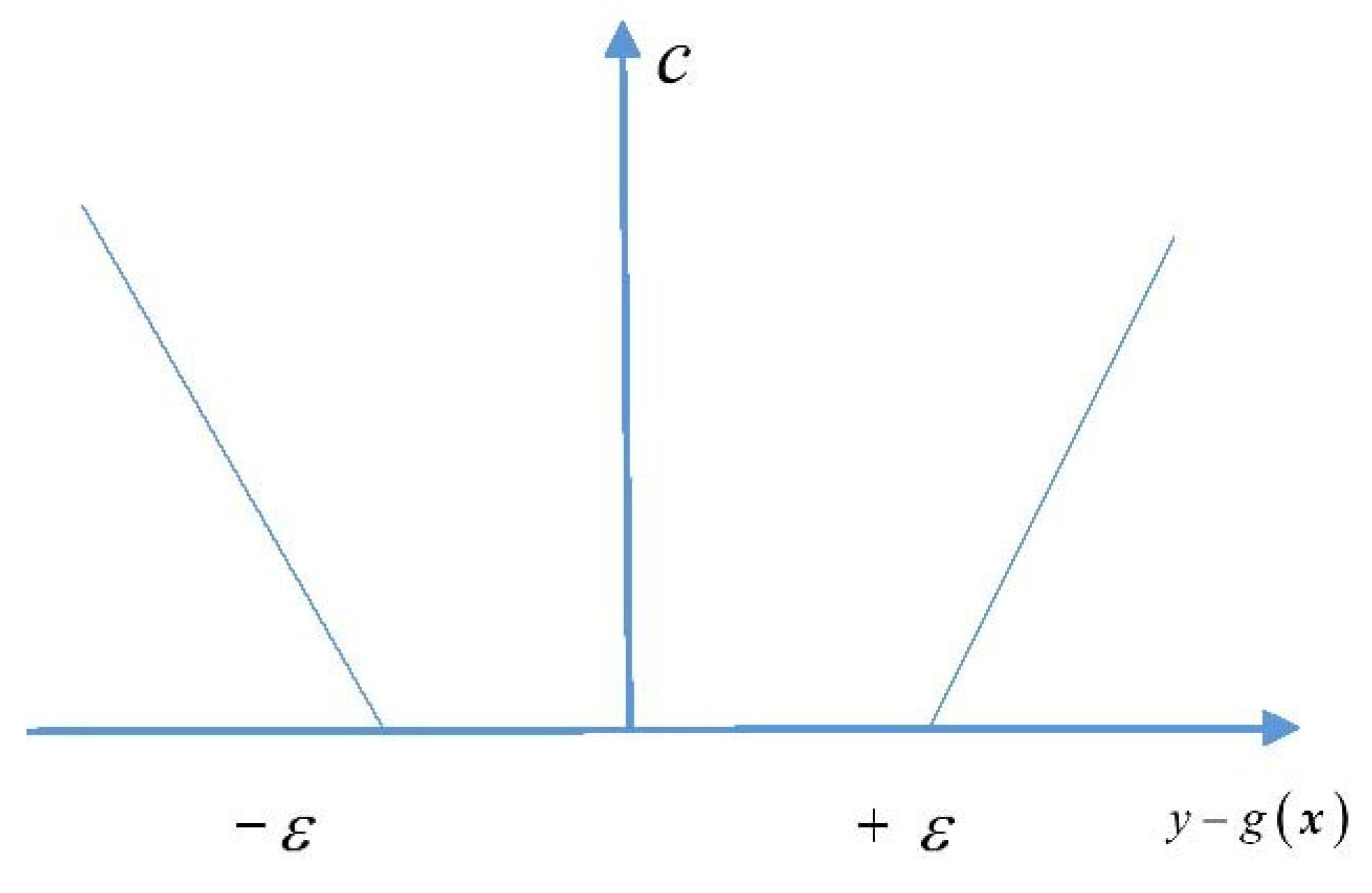
The kernel function effects the transformation from space $R^n$ to Hilbert space $\Phi :x\to \Phi \left(x\right)$, $\Phi :x^{\prime }\to \Phi \left(x^{\prime }\right)$ i.e., it replaces the inner product in the original space, $K\left(x,x^{\prime }\right)=\left(\Phi \left(x\right)\cdot \Phi \left(x^{’}\right)\right)$. The insensitive loss function. $c$ is as given below:

$$c\left(x,y,g\left(x\right)\right)=\{\begin{array}{c}0,\\ \left|y-g\left(x\right)\right|-\epsilon ,\end{array}\begin{array}{c}\left|y-g\left(x\right)\right|<\epsilon \\ \mathrm{others}\end{array}$$

(6)

$\epsilon$ is a positive number selected in advance and when the difference between the observed value $y$ and predicted value $g\left(x\right)$ of $\epsilon$ point does not exceed a given value set in advance, the predicted value $g\left(x\right)$ at that point is considered to be lossless, although the predicted value $g\left(x\right)$ and the observed value $y$ may not be exactly equal. An image of the insensitive loss function $\epsilon$ is shown in Figure 2.

Step 3: Construct and solve convex quadratic programming

$$\begin{array}{l}\underset{\begin{array}{c}{\alpha }^{(*)}\in R^{2l}\\ {\alpha }_i\end{array}}{\min }\hspace{0.17em}\hspace{0.17em}\hspace{0.17em}\frac{1}{2}{\displaystyle \sum _{i,j=1}^l\left({\alpha }_i^{*}-{\alpha }_i\right)\left({\alpha }_j^{*}-{\alpha }_j\right)K\left(x_{\mathrm{i}},x_{\mathrm{j}}\right)}+\epsilon {\displaystyle \sum _{i=1}^l\left({\alpha }_i^{*}+{\alpha }_i\right)}-{\displaystyle \sum _{i=1}^l{y}_i\left({\alpha }_i^{*}-{\alpha }_i\right)}\\ \mathrm{s}.\mathrm{t}.\hspace{0.17em}\hspace{0.17em}\hspace{0.17em}\hspace{0.17em}\hspace{0.17em}{\displaystyle \sum _{i=1}^l\left({\alpha }_i^{*}-{\alpha }_i\right)}=0\\ \hspace{0.17em}\hspace{0.17em}\hspace{0.17em}\hspace{0.17em}\hspace{0.17em}\hspace{0.17em}\hspace{0.17em}0\le {\alpha }_i^{(*)}\le C,i=1,\cdots ,l\end{array}$$

(7)

The solution is given by the expression ${\overline{\mathrm{a}}}^{(*)}={\left(\begin{array}{ccc}{\overline{\alpha }}_1,{\overline{\alpha }}_1^{*},& \cdots ,& {\overline{\alpha }}_l,{\overline{\alpha }}_l^{*}\end{array}\right)}^{{\rm T}}$.

Step 4: Calculation of $\overline{b}$: Select the component ${\overline{\alpha }}_j$ or ${\overline{\alpha }}_k^{*}$ of ${\overline{\mathrm{a}}}^{(*)}$ in the open interval $\left(0,C\right)$. If ${\overline{\alpha }}_j$ is selected, then

$$\overline{b}=y_j-{\displaystyle \sum _{i=1}^l\left({\overline{\alpha }}_i^{*}-{\overline{\alpha }}_i\right)K\left(x_{\mathrm{i}},x_{\mathrm{j}}\right)}+\epsilon$$

(8)

and if ${\overline{\alpha }}_k^{*}$ is selected, then

$$\overline{b}=y_k-{\displaystyle \sum _{i=1}^l\left({\overline{\alpha }}_i^{*}-{\overline{\alpha }}_i\right)K\left(x_{\mathrm{i}},x_{\mathrm{k}}\right)}-\epsilon$$

(9)

Step 5: Construct the decision function

$$y=g\left(x\right)={\displaystyle \sum _{i=1}^l\left({\overline{\alpha }}_i^{*}-{\overline{\alpha }}_i\right)K\left(x_{\mathrm{i}},x\right)}+\overline{b}$$

(10)

3.2. Construction of Mixed Kernel Function

The assessment of the learning performance and generalization performance of the SVM depends on the selection of the kernel functions. Two types of kernel functions are widely used: (1) the $q$ polynomial kernel function, $K\left(x,x^{\prime }\right)={\left[\left(x\cdot x^{\prime }\right)+1\right]}^q,\left(q=1,2,\cdots \right)$ and (2) the Gaussian radial basis kernel function, $K\left(x,x^{\prime }\right)=\exp \left(-{\Vert x-x^{\prime }\Vert }^2/{\sigma }^2\right),\left(\sigma >0\right)$ [35].

The polynomial kernel function is a global kernel function with strong generalization ability but weak learning ability [36], whereas the Gaussian radial basis kernel function is a local kernel function with strong learning ability but weak generalization ability. It is difficult to obtain good results in regression forecasting [37] by using only a single kernel function. Moreover, there are certain limitations in using the SVM with a single kernel function to predict the non-linear change in the data of the number of allocated containers of the container ship for one voyage.

A mixed kernel function is a combination of single kernel functions, integrating their advantages while compensating for the drawbacks, to obtain a performance that can not be achieved by a single kernel function. The mixed function proposed in this study is based on a comprehensive consideration of the local and global kernel functions. According to Mercer’s theorem, the convex combination of two Mercer kernel functions is a Mercer kernel function, and thus, the following kernel functions given by Equation (11) are also kernel functions:

$$K\left(x,x^{\prime }\right)=\left(1-\rho \right)\exp \left(-{\Vert x-x^{\prime }\Vert }^2/{\sigma }^2\right)+\rho {\left[\left(x\cdot x^{\prime }\right)+1\right]}^q$$

(11)

where $0<\rho <1$, and $\rho$ is the weight adjustment factor.

In Equation (11), the flexible combination of the radial basis kernel function and polynomial kernel function is obtained by adjusting the value of $\rho$ [38]. When $\rho >0.5$, the polynomial kernel function is dominant and the mixed function shows strong generalization ability and when $\rho <0.5$, the radial basis kernel function is dominant, and the mixed kernel function shows strong learning ability. Therefore, the mixed kernel function SVM exhibits a better overall performance in predicting the number of allocated containers of the container ship for one voyage.

3.3. Parameter Optimization

The prediction accuracy of the mixed kernel function SVM is related to the insensitive loss parameter $\epsilon$, penalty parameter $C$, polynomial kernel function parameter $q$, width of the radial basis kernel function $\sigma$, and the weight adjustment factor $\rho$. At present, when the SVM is used for regression fitting prediction, the methods for determining the penalty parameters and kernel parameters mainly include the experimental method [39], grid method [40], ant colony algorithm [41], and particle swarm algorithm [42]. Although the relevant parameters for the experiment can be obtained by a large number of calculations, the efficiency is low and the selected parameters do not necessarily measure up to the global optimum. By setting the step size for the data within the parameter range, the grid method sequentially optimizes and compares the results to obtain the optimal parameter values. If the parameter range is large and the set step size is small, the time spent in the optimization process is too long, and the result obtained may be a local optimum. As a general stochastic optimization method, the ant colony algorithm has achieved good results in a series of combinatorial optimization procedures. However, the parameter setting in the algorithm is usually determined by experimental methods resulting in a close interdependence between the optimization performance of the method and human experience, making it difficult to optimize the performance of the algorithm. Due to the loss of diversity of species in search space, the particle swarm algorithm leads to premature convergence and poor local optimization ability [43,44]. Therefore, it is of great importance to apply the appropriate optimization algorithm for optimal combinatorial results of the parameters of the support vector of the mixed kernel functions to obtain the SVM with the best performance [45], which will ensure an accurate prediction of the number of allocated containers of the container ship for one voyage.

The GA [46] is the most widely used successful algorithm in intelligent optimization. It is a general optimization algorithm with a relatively simple coding technique using genetic operators. Its optimization is not restrained by restrictive conditions and its two most prominent features are implicit parallelism and global solution space search. Therefore, GA is used in this study to optimize the parameter combination $\left(\begin{array}{ccccc}\epsilon & C& q& \sigma & \rho \end{array}\right)$ consisting of 5 parameters.

In the optimization of the SVM parameter combination of the mixed kernel function by using GA, each chromosome represents a set of parameters and the chromosome species search for the optimal solution through the GA (including interlace operation and mutation operation) and strategy selection. As the objective of optimizing the SVM parameters of the mixed kernel function is to obtain better prediction accuracy, the mixed kernel function $\left(\begin{array}{ccccc}{\epsilon }_n& C_n& q_n& {\sigma }_n& {\rho }_n\end{array}\right)$ SVM model is trained and then tested by 5 × cross validation. Proportional selection is the selection strategy adopted in this study. After the probability is obtained, the roulette wheel is used to determine the selection operation and hence, the fitness function is defined as the reciprocal of the prediction error of the mixed kernel function SVM as given below:

$$F=1/\frac{1}{5}{\displaystyle \sum _{i=1}^5\left[\frac{1}{m}{\displaystyle \sum _{j=1}^{NP}{\left({\widehat{P}}_{ij}-P_{ij}\right)}^2}\right]}$$

(12)

where NP is the number of data in each sample subset, ${\widehat{P}}_{ij}$ is the predicted value, and $P_{ij}$ is the actual value. Thus, the chromosome with the minimum fitness function value in the whole chromosome swarm as well as its index among the chromosome swarm is determined.

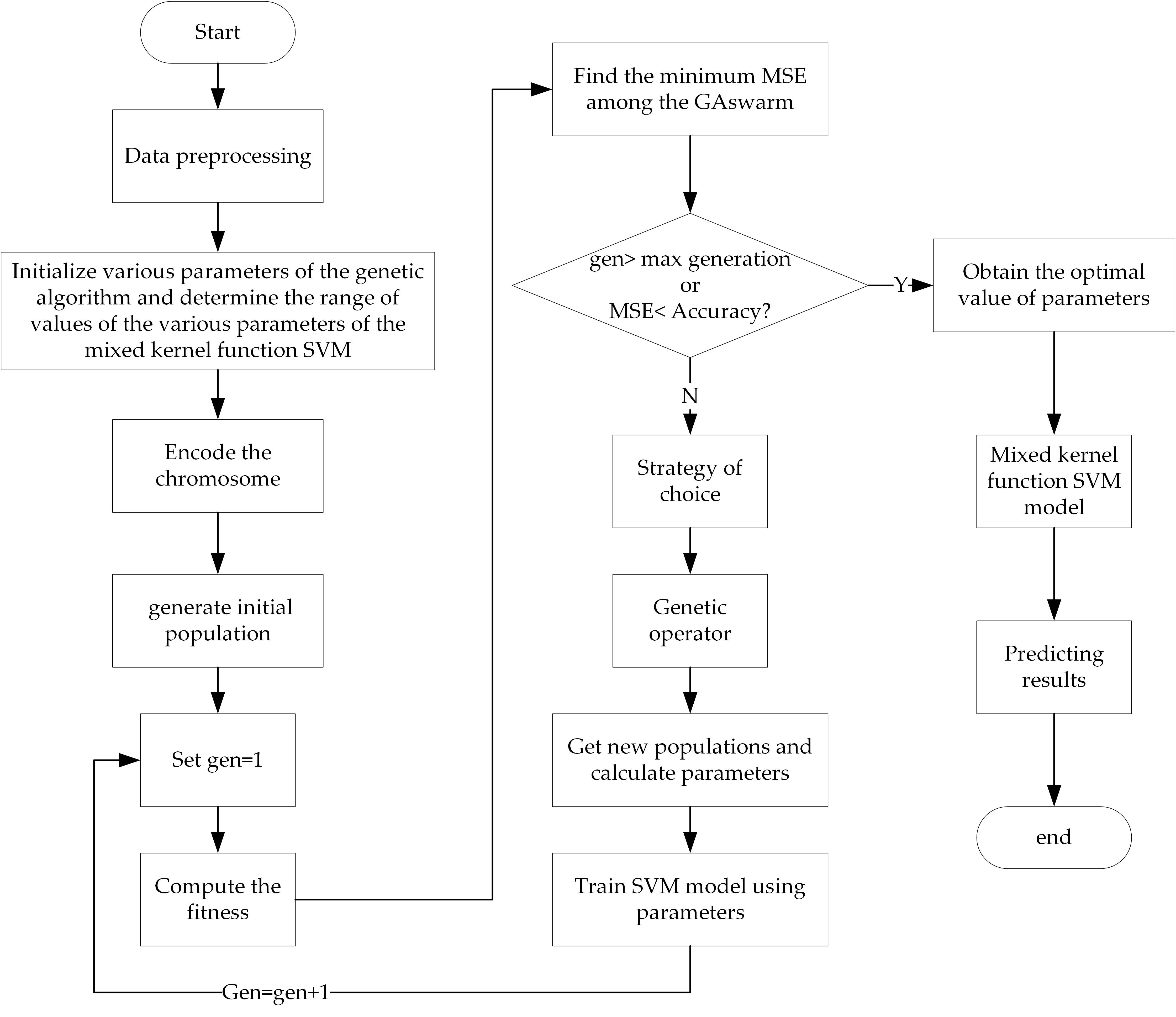
The step-wise process of optimizing the parameters $\left(\begin{array}{ccccc}\epsilon & C& q& \sigma & \rho \end{array}\right)$ by using GA is given below and the flow diagram is illustrated in Figure 3.

Step 1: Data preprocessing, mainly including normalization processing and dividing the sample data into training data and test data.

Step 2: Initialize various parameters of the GA and determine the range of values of the various parameters of the mixed kernel function SVM. First, set the maximum number of generations (gen = 50), population size (NP), individual length, generation gap (GGAP = 0.95), crossover rate ($P_x$ = 0.7), and mutation rate ($P_m$ = 0.01). Next, set the range of the parameters $\left(\begin{array}{ccccc}\epsilon & C& q& \sigma & \rho \end{array}\right)$. Since this optimization model (GA) is not the highlight in this paper, the criteria for parameter selection, i.e., gen = 50, GGAP = 0.95, $P_x$ = 0.7, $P_m$ = 0.01, are not given here in detail, and the selection of parameters is based on the empirical practice provided in reference [46]. Moreover, the setting of these parameters has achieved good results in this paper.

Step 3: Encode the chromosomes and generate the initial population. Encode the chromosomes in a 7-bit binary and randomly generate NP individuals ($s_1,s_2,\cdots ,s_{NP}$) to form the initial population $S$ ($S=\left\{s_1,s_2,\cdots ,s_{NP}\right\}$).

Step 4: Calculate the fitness of each individual. Find the minimum mean squared error (MSE) among the GA swarm.

Step 5: If the termination condition is satisfied, the individual with the greatest fitness in $S$ is the most sought after result which is then decoded to obtain the optimal parameters $\left(\begin{array}{ccccc}\epsilon & C& q& \sigma & \rho \end{array}\right)$. The optimized parameters $\left(\begin{array}{ccccc}\epsilon & C& q& \sigma & \rho \end{array}\right)$ are used to train the SVM model, which generates the prediction result. This marks the end of the algorithm.

Step 6: Proportional selection is performed by the roulette wheel method, and the selected probability is calculated by using Equation (13). 95% of the individuals are selected from the parent population $S$ to form the progeny population $S_1$ (as GGAP = 0.95). Genetic operations are performed on new populations, crossover operations are performed using single tangent points, and mutation operations are performed using basic bit variation operations.

$$P_i=F_i/{\displaystyle \sum _{i=1}^{NP}{F}_i}$$

(13)

Step 7: Subsequent to the genetic manipulation, a new population $S_3$ is obtained and the parameters $\left(\begin{array}{ccccc}\epsilon & C& q& \sigma & \rho \end{array}\right)$ are calculated. The SVM model is then trained with the new parameters.

Step 8: $S_3$ is now considered to be the new generation population, i.e., $S$ is replaced by $S_3$, gen = gen + 1, and the process is repeated from step 4.

4. Example Analysis

This study set $X_0=\left(\begin{array}{cccccc}{x}_0\left(1\right),& x_0\left(2\right),& \cdots ,& x_0\left(k\right),& \cdots ,& x_0\left(n\right)\end{array}\right)$ as the reference sequence (i.e., the number of containers for a voyage (the study object)) and $X_i=\left(\begin{array}{cccccc}{x}_i\left(1\right),& x_i\left(2\right),& \cdots ,& x_i\left(k\right),& \cdots ,& x_i\left(n\right),\end{array}\right)\left(i=1,2,\cdots ,m\right)$ as the comparative sequence (i.e., factors influencing the number of allocated containers for one voyage during the voyage period). Parameter n represents the number of samples and m represents the number of influencing factors; in this study, m = 9. GRA was applied. The weighted influencing factors were then used as the input of the mixed kernel function SVM.

4.1. Data Samples

To establish a model for forecasting the number of containers allocated to a container ship for one voyage, factors influencing the number of allocated containers must be analyzed and an index system for forecasting the number of allocated containers must be established. Numerous factors influence the number of containers allocated to a container ship for one voyage; such factors include the port of call, the company (fleet) to which the ship belongs, and the ship itself. A predictive index for forecasting container allocation is outlined as follows ($i$ represents the $i\mathrm{th}$ influencing factor, $i=1,2,\cdots ,m$):

(1)

$X_1$, local GDP of the region in which the port of call is located, which can be calculated on the basis of the formula actual amount/100 million yuan;

(2)

$X_2$, changes in port industrial structures, which can calculated according to the percentage occupied by the tertiary industry;

(3)

$X_3$, completeness of the collection and distribution system, which can calculated according to the actual annual throughput of containers per million twenty-foot equivalent units (TEU) at the port of call;

(4)

$X_4$, company’s capacity, which can be calculated according to the actual number of containers/10,000 TEU;

(5)

$X_5$, inland turnaround time of containers, which can be calculated according to the actual number of days;

(6)

$X_6$, seasonal changes in cargo volume, which can be calculated as a percentage;

(7)

$X_7$, quantity of containers handled by the company, which can be calculated according to the actual number of containers/10,000 TEU;

(8)

$X_8$, transport capacity for a single ship, which can be calculated according to the actual number of containers/TEU; and

(9)

$X_9$, full-container-loading rate of the ship, which can be calculated as a percentage.

For different shipping lines, ports, and container ships, collecting actual data pertaining to the nine aforementioned factors is difficult. Moreover, information on some of these factors is treated as confidential by company or ship management teams. To verify the practicality of the model, this study simulated a set of data. To ensure that the sample data were reasonable and approached real situations, this study sought information from the literature [8,9], in addition to consulting the department heads of shipping lines and stowage operators.

The selected training samples are presented in

Table 1. Training samples.

No.	${\mathit{X}}_1$	${\mathit{X}}_2$	${\mathit{X}}_3$	${\mathit{X}}_4$	${\mathit{X}}_5$	${\mathit{X}}_6$	${\mathit{X}}_7$	${\mathit{X}}_8$	${\mathit{X}}_9$	${\mathit{X}}_0$
1	2395	75	2461	10.3	11	20	21	5200	77	1100
2	27,689	66	776	85	38	10	170	1700	85	279
3	29,960	77	2521	102.3	10	15	230	4700	69	1739
4	29,841	82	4123	162	49	13	201	3410	64	177
5	13,562	63	2357	68.9	39	20	150	1200	73	110
6	17,369	59	2037	60.3	22	26	120	800	62	205
7	14,650	71	1521	59	13	29	147	2800	73	347
8	30,550	58	798	47.7	26	15	128	3600	88	561
9	25,103	54	567	110.3	13	10	235	2000	65	850
10	14,650	65	668	85.6	25	12	164	2590	86	496
11	14,023	49	732	77.7	16	30	139	2810	59	594
12	19,776	67	651	56	30	21	98	1400	71	350

.

4.2. Determining the Weight of Influencing Factors

As indicated by the data in the table, the order of magnitude of the sequences was quite different, and the two sequences were standardized using Equation (1). The correlation between each influencing factor and the number of containers allocated to the container ship for one voyage was calculated using Equations (2), (3) and(4), and the calculation results are presented in

Table 2. Correlation between each influencing factor and study object.

Factors	Relevance	Factors	Relevance	Factors	Relevance
$X_1$	0.1669	$X_4$	0.1773	$X_7$	0.1770
$X_2$	0.6672	$X_5$	0.3998	$X_8$	0.8345
$X_3$	0.7084	$X_6$	0.6206	$X_9$	0.6232

.

As shown in Table 2, the correlation degrees of $X_1$, $X_4$, and $X_7$ were all approximately 0.17, indicating that the three influencing factors had the lowest effect on the number of allocated containers for one voyage and could be ignored. The correlation degree of $X_5$ was 0.3998, signifying that this factor had little effect on the number of allocated containers for one voyage; the correlation degrees of $X_2$, $X_6$, $X_3$, and $X_9$ were higher than 0.6, indicating that these three factors had a significant effect on the number of allocated containers for one voyage. However, the correlation degree of $X_8$ was 0.8345, signifying that this factor had the greatest effect on the number of allocated containers for one voyage. The weight of each influencing factor was calculated using Equation (5), and

Table 3. Weight of each influencing factor.

Factors	Weight	Factors	Weight	Factors	Weight
$X_1$	0.038	$X_4$	0.041	$X_7$	0.040
$X_2$	0.153	$X_5$	0.091	$X_8$	0.191
$X_3$	0.162	$X_6$	0.142	$X_9$	0.142

shows the results.

As shown in Table 3, the weight values of $X_1$, $X_4$, and $X_7$ were relatively low (all lower than 0.091), and the weight values of the other influencing factors were higher than 0.14, with no significant difference. This is mainly because the other factors had greater effects on the number of allocated containers for one voyage, and their weight values were scattered.

4.3. Prediction of Number of Allocated Containers for One Voyage Using Mixed Kernel SVM

Weighted factors could be derived by multiplying the influencing factors by the corresponding weights:

$${\overline{X}}_i=w_i{X}_i,\hspace{0.17em}\hspace{0.17em}\hspace{0.17em}i=1,2,\cdots ,9$$

(14)

where ${\overline{X}}_i$ is the weighted factor influencing the number of allocated containers for one voyage. When ${\overline{X}}_i$ in the composition vector $Q={\left[{\overline{X}}_1,{\overline{X}}_2,\cdots ,{\overline{X}}_9\right]}^{{\rm T}}$ was considered the input variable and $X_0$ was considered the corresponding output variable, a mixed kernel SVM for predicting the number of allocated containers for one voyage was constructed.

All data were normalized to the interval $\left[0,1\right]$. The data presented in Table 1 served as training samples, whereas those presented in

Table 4. Test samples.

No.	${\mathit{X}}_1$	${\mathit{X}}_2$	${\mathit{X}}_3$	${\mathit{X}}_4$	${\mathit{X}}_5$	${\mathit{X}}_6$	${\mathit{X}}_7$	${\mathit{X}}_8$	${\mathit{X}}_9$	${\mathit{X}}_0$
1	4365	76	1596	24	13	18	43	5400	72	1250
2	23,560	69	882	87	29	12	185	1900	83	900
3	9841	81	2143	112	12	17	251	4580	70	750
4	25,590	74	4265	159	50	14	211	3390	66	500
5	18,763	62	1983	73	41	21	163	1080	74	310

served as test samples.

The GA control parameters were as follows: $\epsilon$, $C$, $q$, $\sigma$, $\rho$ were binary coded, with the optimal ranges being set to $\epsilon \in \left[{10}^{-10},{10}^{-1}\right]$, $C\in \left[0,50\right]$, $q\in \left[0,20\right]$, $\sigma \in \left[0,500\right]$, and $\rho \in \left[0,1\right]$, respectively. The series size was 50, maximum evolution algebra was 50 generations, crossover probability was 0.7, mutation probability was 0.01, and the judgment termination accuracy was ${10}^{-4}$.

This study applied MSE, mean absolute percentage error ($e_{\mathrm{MAPE}}$), and correlation coefficients ($R$) to evaluate the predictive performance of the model. $R$ was set to the interval $\left[0,1\right]$. Lower MSE and $e_{MRE}$ values and $R$ values approaching 1 were considered to indicate higher model predictive performance.

$$\begin{array}{c}\mathrm{MSE}=\frac{1}{l}{\displaystyle \sum _{i=1}^l{\left({\overline{y}}_i-y_i\right)}^2}\\ e_{\mathrm{MAPE}}=\frac{1}{l}{\displaystyle \sum _{i=1}^l\left|\frac{{\overline{y}}_i-y_i}{y_i}\right|}\cdot 100\%\\ R=\sqrt{\frac{{\left(l{\displaystyle \sum _{i=1}^l{\overline{y}}_i{y}_i}-{\displaystyle \sum _{i=1}^l{\overline{y}}_i}{\displaystyle \sum _{i=1}^l{y}_i}\right)}^2}{\left(l{\displaystyle \sum _{i=1}^l{\overline{y}}_i^2}-{\left({\displaystyle \sum _{i=1}^l{\overline{y}}_i}\right)}^2\right)\left(l{\displaystyle \sum _{i=1}^l{y}_i^2}-{\left({\displaystyle \sum _{i=1}^l{y}_i}\right)}^2\right)}}\end{array}$$

(15)

where $l$ is the number of samples, $y_i\left(i=1,2,\cdots l\right)$ is the real value of the $i\mathrm{th}$ sample, and ${\overline{y}}_i\left(i=1,2,\cdots l\right)$ is the predicted value of the $i\mathrm{th}$ sample.

4.4. Simulation Results and Analysis

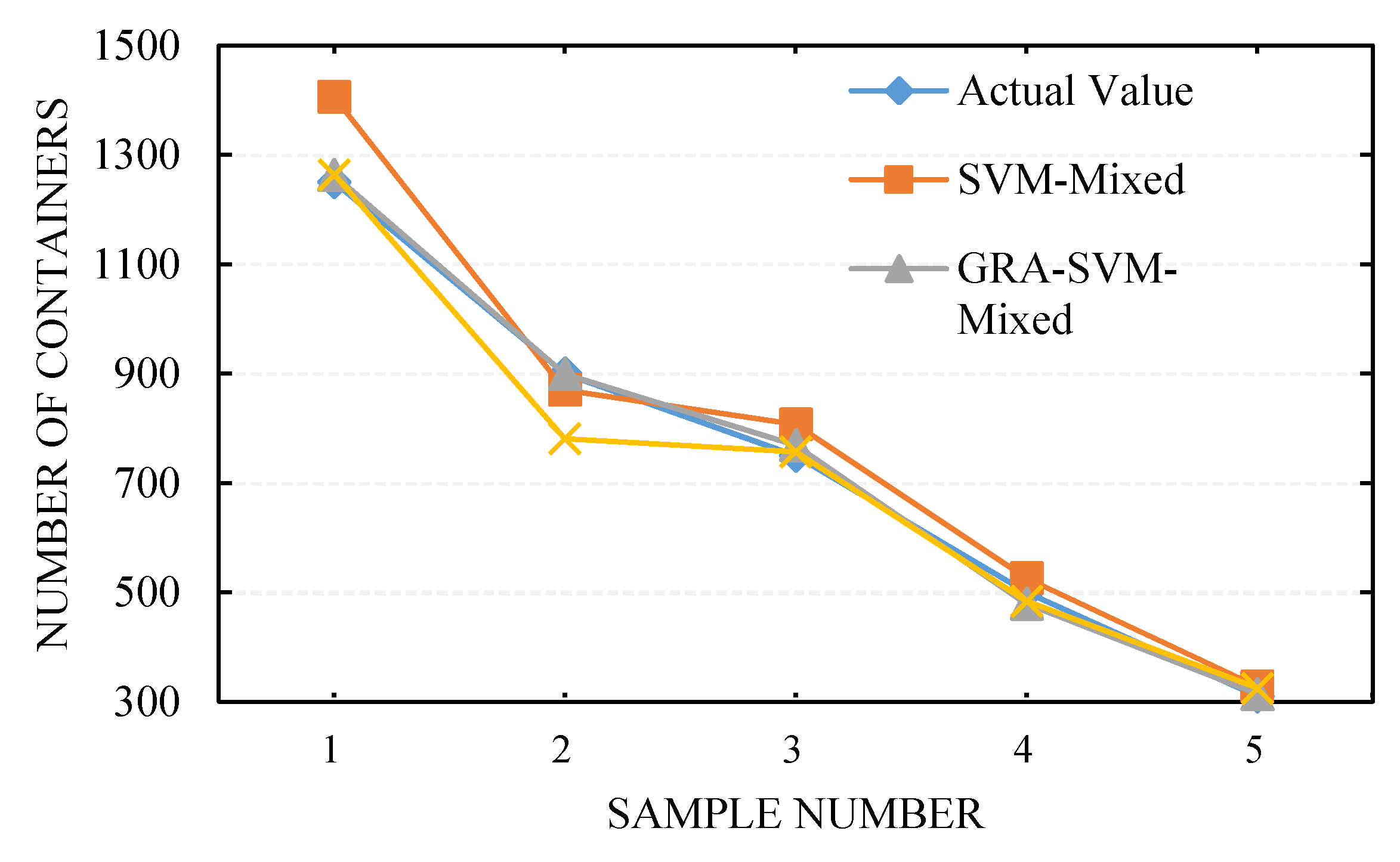
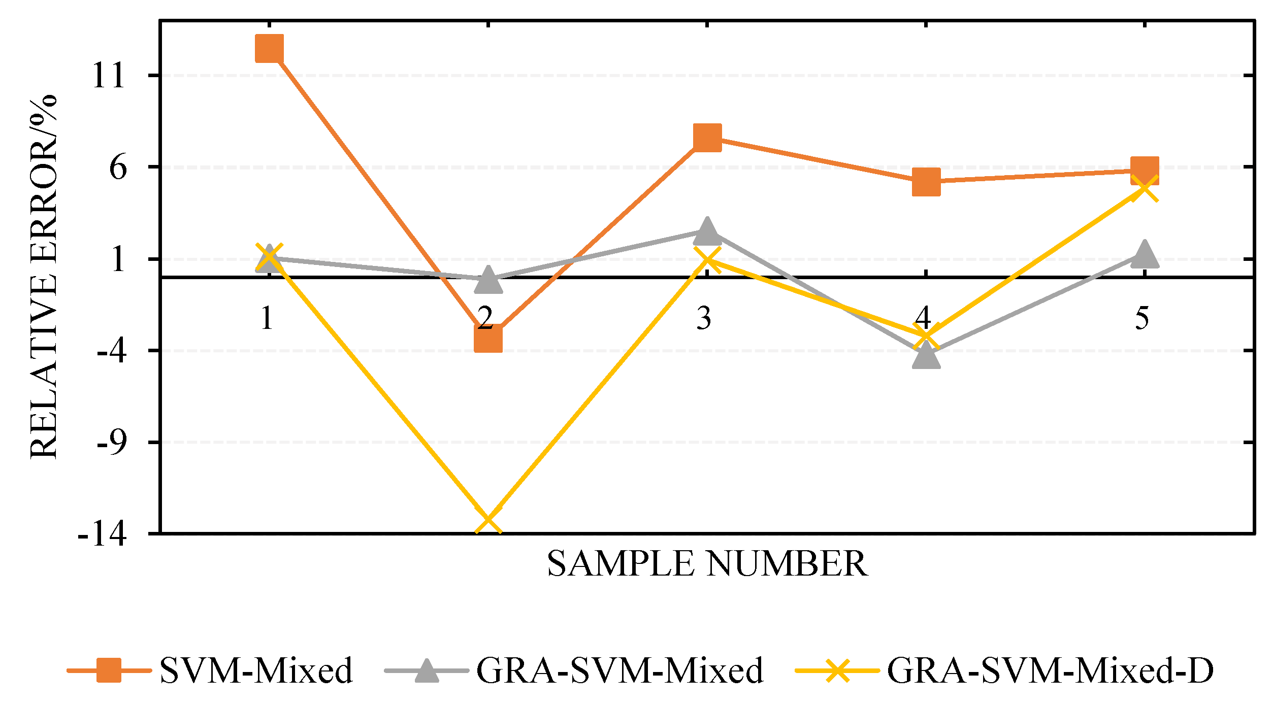
The parameters $\left(\begin{array}{ccccc}\widehat{\epsilon }& \widehat{C}& \widehat{q}& \widehat{\sigma }& \widehat{\rho }\end{array}\right)$ of the mixed kernel SVM were obtained through GA optimization, which was used to establish the mixed kernel SVM model and predict the number of voyage containers in the test samples. The various input variables affected the predictive performance of the model, and the specific results are presented in

Table 5. Comparison of predictions for different input variables.

No.	Actual	SVM-Mixed		GRA-SVM-Mixed		GRA-SVM-Mixed-D
		Predictive	Relative Error	Predictive	Relative Error	Predictive	Relative Error
1	1250	1406	12.48	1263	1.04	1264	1.12
2	900	870	−3.33	899	−0.11	781	−13.22
3	750	807	7.60	769	2.53	757	0.93
4	500	526	5.20	479	−4.20	484	−3.20
5	310	328	5.81	314	1.29	325	4.84
MSE		5897		197.6		2977.4
$e_{\mathrm{MAPE}}$		6.88		1.83		4.66
$R$		0.9908		0.9993		0.9877

and Figure 4.

The calculation results revealed that under the same model parameters, changing the input variables engendered different predictive performance levels. The input variables of the GRA-SVM-MIXED model were constituted by all the weighted influencing factors (see Table 3 for weight values); the input variables of the SVM-Mixed model were constituted by all the unweighted factors. For the GRA-SVM-Mixed-D model, influencing factors with correlation degrees lower than 0.6 were eliminated, and the remaining influencing factors were considered the model input variables. As presented in Table 5 and Figure 4, the maximum (minimum) error, MSE, and $e_{MRE}$ of the GRA-SVM-Mixed model were significantly lower than those of the GRA-SVM-mixed-D and SVM-mixed models; in addition, the GRA-SVM-Mixed model had the highest correlation coefficient $R$, indicating that the GRA-SVM-mixed model exhibited higher predictive performance than did the other two models. As illustrated in Figure 4 and Figure 5, the GRA-SVM-Mixed model provided closer predictions to the actual values in the test sample than did the other two models, and no large inflection point was observed. Furthermore, the maximum relative error observed for the GRA-SVM-Mixed model was −4.2%, minimum error was −0.11%, and correlation coefficient was as high as 0.9993, showing higher predictive performance. This is because after the influencing factors were subjected to gray correlation analysis, different weights were assigned to the input variables, the intrinsic correlation characteristics between the influencing factors and the number of allocated containers for one voyage were fully explored, and the influencing factors with low correlation degree were eliminated. The maximum relative error observed for the GRA-SVM-Mixed-D model was −13.22%, minimum relative error was 0.93%, and correlation coefficient was 0.9877, which was the smallest among the three models, and this could be attributed to the elimination of influencing factors with low correlation degrees. Although eliminating influencing factors with low correlation degrees could simplify the structure of the prediction model, the predictive performance of the model was relatively poor because it could not reflect the differences among the factors.

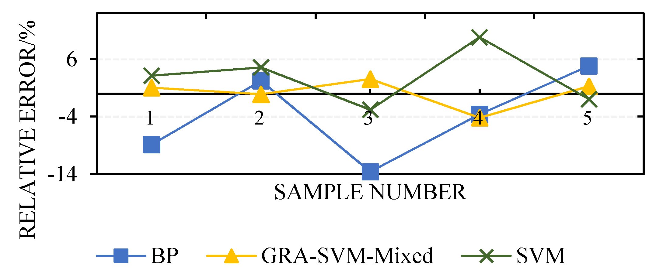
On the basis of the same sample in this study, the methods in [8,9] were used to construct models for predicting the number of allocated containers for one voyage, which were denoted as BP and SVM, respectively. As illustrated in Figure 6, the GRA-SVM-Mixed model had more stable prediction results and more accurate predictions than did the BP and SVM models. The test indicators in

Table 6. Comparison of predictive performance of different models.

No.	Relative Error
	BP	SVM	GRA-SVM-Mixed
1	−8.88	3.12	1.04
2	2.22	4.56	−0.11
3	−13.6	−2.80	2.53
4	−3.6	9.80	−4.20
5	4.84	−0.97	1.29
MES	4734.8	1210.6	197.6
$R$	0.9883	0.9969	0.9993
t/s	57.63	45.61	27.53

further confirm these findings. As presented in Table 6, all the three models could provide good prediction results and satisfactory MSE and $e_{\mathrm{MAPE}}$ values. The GRA-SVM-Mixed model exhibited higher predictive performance. Moreover, the GRA-SVM-Mixed model was determined to have significant advantages over the other two models from a timesaving perspective.

The maximum relative errors of the predictions of the three models were −13.6%, 2.53%, and 9.8%, and the minimum relative errors were −2.22%, −0.11%, and −0.97%. The predictive performance of a model can be expressed by the MSE and correlation coefficient $R$. As shown in Table 6, the MSE of the GRA-SVM-Mixed model was 197.6 and the $R$ was 0.9993, which was closer to 1 compared with those of the other two models. This is because under small samples, the BP neural network model adopts empirical risk minimization, whereas the minimum expected risk cannot be guaranteed. Moreover, the BP neural network model can only guarantee convergence to a certain point in the optimization process and cannot derive a global optimal solution. By contrast, the SVM model adopts structural risk minimization and VC dimension theory, which not only minimizes the structural risk but also minimizes the boundary of the VC dimension under a small sample, effectively narrowing the confidence interval, thus achieving the minimum expected risk and improving the generalization ability and promotion ability of the model. The GRA-SVM-Mixed model applies parameter $\rho$ to adjust the flexible use of radial basis and polynomial kernel functions in order to improve its robustness and generalization ability. In addition, the model applies gray correlation analysis for weighting input variables, strengthening the internal feature space structure and reflecting the differences among influencing factors. In this study, this model exhibited good performance in predicting the number of containers allocated to a container ship for one voyage.

5. Conclusions

This paper proposes a model for predicting the number of containers allocated to a container ship for one voyage. First, GRA theory is applied to determine the correlation between influencing factors and the forecasting sequence. Subsequently, different weights are allocated to each influencing factor to reflect their differences and highlight their internal characteristics. The weighted influencing factors serve as the input variables of the SVM prediction model, and a radial basis kernel function and polynomial kernel function are applied to improve the generalization ability and promotion ability of the SVM model. Finally, a GA is used to optimize the SVM parameters, and samples are trained using the optimized parameters to improve the predictive performance of the model. Simulations revealed that compared with an SVM model with a single kernel function and without gray correlation processing, the proposed model exhibited higher performance, with the minimum relative error rates being −0.11% and −0.97%, respectively. Additionally, compared with a BP neural network model, the GRA-SVM-Mixed model exhibited superior generalization ability, according to a relative error analysis. Accordingly, the proposed model provides an effective method for predicting the number of containers allocated to a container ship for one voyage.

References

- Helo, P.; Paukku, H.; Sairanen, T. Containership cargo profiles, cargo systems, and stowage capacity: Key performance indicators. Marit. Econ. Logist. 2018, 1–21. [Google Scholar] [CrossRef]
- Gosasang, V.; Chandraprakaikul, W.; Kiattisin, S. An application of neural networks for forecasting container throughput at Bangkok port. In Proceedings of the World Congress on Engineering, London, UK, 30 June–2 July 2010; pp. 137–141. [Google Scholar]
- Iris, Ç.; Pacino, D.; Ropke, S.; Larsen, A. Integrated berth allocation and quay crane assignment problem: Set partitioning models and computational results. Transp. Res. Part E Logist. Transp. Rev. 2015, 81, 75–97. [Google Scholar] [CrossRef] [Green Version]
- Jiang, J.; Wang, H.; Yang, Z. Econometric analysis based on the throughput of container and its main influential factors. J. Dalian Marit. Univ. 2007, 1. [Google Scholar] [CrossRef]
- Chou, C. Analysis of container throughput of major ports in Far Eastern region. Marit. Res. J. 2002, 12, 59–71. [Google Scholar] [CrossRef]
- Meersman, H.; Steenssens, C.; Van de Voorde, E. Container Throughput, Port Capacity and Investment; SESO Working Papers 1997020; University of Antwerp, Faculty of Applied Economics: Antwerpen, Belgium, 1997. [Google Scholar]
- Karsten, C.V.; Ropke, S.; Pisinger, D. Simultaneous optimization of container ship sailing speed and container routing with transit time restrictions. Transp. Sci. 2018, 52, 769–787. [Google Scholar] [CrossRef]
- Weiying, Z.; Yan, L.; Zhuoshang, J. A Forecast Model of the Number of Containers for Containership Voyage Based on SVM. Shipbuild. China 2006, 47, 101–107. [Google Scholar]
- Li, S. A forecast method of safety container possession based on neural network. Navig. China 2002, 3, 56–60. [Google Scholar]
- Grudnitski, G.; Osburn, L. Forecasting S&P and gold futures prices: An application of neural networks. J. Futures Mark. 1993, 13, 631–643. [Google Scholar] [CrossRef]
- White, H. Connectionist nonparametric regression: Multilayer feedforward networks can learn arbitrary mappings. Neural Netw. 1990, 3, 535–549. [Google Scholar] [CrossRef]
- Chakraborty, K.; Mehrotra, K.; Mohan, C.K.; Ranka, S. Forecasting the behavior of multivariate time series using neural networks. Neural Netw. 1992, 5, 961–970. [Google Scholar] [CrossRef] [Green Version]
- Lapedes, A.; Farber, R. Nonlinear signal processing using neural networks: Prediction and system modelling. In Proceedings of the IEEE International Conference on Neural Networks, San Diego, CA, USA, 21 June 1987. [Google Scholar]
- Yu, J.; Tang, G.; Song, X.; Yu, X.; Qi, Y.; Li, D.; Zhang, Y. Ship arrival prediction and its value on daily container terminal operation. Ocean Eng. 2018, 157, 73–86. [Google Scholar] [CrossRef]
- Hsu, C.; Huang, Y.; Wong, K.I. A Grey hybrid model with industry share for the forecasting of cargo volumes and dynamic industrial changes. Transp. Lett. 2018, 1–12. [Google Scholar] [CrossRef]
- Vapnik, V.N. An overview of statistical learning theory. IEEE Trans. Neural Netw. 1999, 10, 988–999. [Google Scholar] [CrossRef] [PubMed]
- Cortes, C.; Vapnik, V. Support-vector networks. Mach. Learn. 1995, 20, 273–297. [Google Scholar] [CrossRef] [Green Version]
- Müller, K.R.; Smola, A.J.; Rätsch, G.; Schölkopf, B.; Kohlmorgen, J.; Vapnik, V. Predicting time series with support vector machines. In Proceedings of the Artificial Neural Networks—ICANN’97, Lausanne, Switzerland, 8–10 October 1997; Springer: Berlin/Heidelberg, Germany, 1997; pp. 999–1004. [Google Scholar] [CrossRef] [Green Version]
- Gunn, S.R. Support vector machines for classification and regression. ISIS Tech. Rep. 1998, 14, 5–16. [Google Scholar]
- Joachims, T. Making Large-Scale SVM Learning Practical. Technical Report, SFB 475. 1998, Volume 28. Available online: http://hdl.handle.net/10419/77178 (accessed on 15 June 1998).
- Smits, G.F.; Jordaan, E.M. Improved SVM regression using mixtures of kernels. In Proceedings of the 2002 International Joint Conference on Neural Networks, Honolulu, HI, USA, 12–17 May 2002; pp. 2785–2790. [Google Scholar] [CrossRef]
- Jebara, T. Multi-task feature and kernel selection for SVMs. In Proceedings of the Twenty-First International Conference on Machine Learning, Banff, AB, Canada, 4–8 July 2004; pp. 329–337. [Google Scholar] [CrossRef]
- Tsang, I.W.; Kwok, J.T.; Cheung, P. Core vector machines: Fast SVM training on very large data sets. J. Mach. Learn. Res. 2005, 6, 363–392. [Google Scholar]
- Lu, Y.L.; Lei, L.I.; Zhou, M.M.; Tian, G.L. A new fuzzy support vector machine based on mixed kernel function. In Proceedings of the 2009 International Conference on Machine Learning and Cybernetics, Baoding, China, 12–15 July 2009; pp. 526–531. [Google Scholar] [CrossRef]
- Xie, G.; Wang, S.; Zhao, Y.; Lai, K.K. Hybrid approaches based on LSSVR model for container throughput forecasting: A comparative study. Appl. Soft Comput. 2013, 13, 2232–2241. [Google Scholar] [CrossRef]
- Deng, J.L. Introduction to Grey System Theory. J. Grey Syst. 1989, 1, 1–24. [Google Scholar]
- Al-Douri, Y.; Hamodi, H.; Lundberg, J. Time Series Forecasting Using a Two-Level Multi-Objective Genetic Algorithm: A Case Study of Maintenance Cost Data for Tunnel Fans. Algorithms 2018, 11, 123. [Google Scholar] [CrossRef]
- Weiwei, W. Time series prediction based on SVM and GA. In Proceedings of the 2007 8th International Conference on Electronic Measurement and Instruments, Xi’an, China, 16–18 August 2007; pp. 307–310. [Google Scholar] [CrossRef]
- Yin, Y.; Cui, H.; Hong, M.; Zhao, D. Prediction of the vertical vibration of ship hull based on grey relational analysis and SVM method. J. Mar. Sci. Technol. 2015, 20, 467–474. [Google Scholar] [CrossRef]
- Kuo, Y.; Yang, T.; Huang, G. The use of grey relational analysis in solving multiple attribute decision-making problems. Comput. Ind. Eng. 2008, 55, 80–93. [Google Scholar] [CrossRef]
- Tosun, N. Determination of optimum parameters for multi-performance characteristics in drilling by using grey relational analysis. Int. J. Adv. Manuf. Technol. 2006, 28, 450–455. [Google Scholar] [CrossRef]
- Shen, M.X.; Xue, X.F.; Zhang, X.S. Determination of Discrimination Coefficient in Grey Incidence Analysis. J. Air Force Eng. Univ. 2003, 4, 68–70. [Google Scholar]
- Yao, X.; Zhang, L.; Cheng, M.; Luan, J.; Pang, F. Prediction of noise in a ship’s superstructure cabins based on SVM method. J. Vib. Shock 2009, 7. [Google Scholar] [CrossRef]
- Huang, C.; Chen, M.; Wang, C. Credit scoring with a data mining approach based on support vector machines. Expert Syst. Appl. 2007, 33, 847–856. [Google Scholar] [CrossRef] [Green Version]
- Duan, K.; Keerthi, S.S.; Poo, A.N. Evaluation of simple performance measures for tuning SVM hyperparameters. Neurocomputing 2003, 51, 41–59. [Google Scholar] [CrossRef] [Green Version]
- Van der Schaar, M.; Delory, E.; André, M. Classification of sperm whale clicks (Physeter Macrocephalus) with Gaussian-Kernel-based networks. Algorithms 2009, 2, 1232–1247. [Google Scholar] [CrossRef] [Green Version]
- Luo, W.; Cong, H. Control for Ship Course-Keeping Using Optimized Support Vector Machines. Algorithms 2016, 9, 52. [Google Scholar] [CrossRef]
- Wei, Y.; Yue, Y. Research on Fault Diagnosis of a Marine Fuel System Based on the SaDE-ELM Algorithm. Algorithms 2018, 11, 82. [Google Scholar] [CrossRef]
- Bian, Y.; Yang, M.; Fan, X.; Liu, Y. A Fire Detection Algorithm Based on Tchebichef Moment Invariants and PSO-SVM. Algorithms 2018, 11, 79. [Google Scholar] [CrossRef]
- Cherkassky, V.; Ma, Y. Practical selection of SVM parameters and noise estimation for SVM regression. Neural Netw. 2004, 17, 113–126. [Google Scholar] [CrossRef] [Green Version]
- Aiqin, H.; Yong, W. Pressure model of control valve based on LS-SVM with the fruit fly algorithm. Algorithms 2014, 7, 363–375. [Google Scholar] [CrossRef]
- Du, J.; Liu, Y.; Yu, Y.; Yan, W. A prediction of precipitation data based on support vector machine and particle swarm optimization (PSO-SVM) algorithms. Algorithms 2017, 10, 57. [Google Scholar] [CrossRef]
- Wang, R.; Tan, C.; Xu, J.; Wang, Z.; Jin, J.; Man, Y. Pressure Control for a Hydraulic Cylinder Based on a Self-Tuning PID Controller Optimized by a Hybrid Optimization Algorithm. Algorithms 2017, 10, 19. [Google Scholar] [CrossRef]
- Liu, D.; Niu, D.; Wang, H.; Fan, L. Short-term wind speed forecasting using wavelet transform and support vector machines optimized by genetic algorithm. Renew. Energy 2014, 62, 592–597. [Google Scholar] [CrossRef]
- Shevade, S.K.; Keerthi, S.S.; Bhattacharyya, C.; Murthy, K.R.K. Improvements to the SMO algorithm for SVM regression. IEEE Trans. Neural Netw. 2000, 11, 1188–1193. [Google Scholar] [CrossRef] [PubMed] [Green Version]
- Holland, J.H. Adaptation in Natural and Artificial Systems: An Introductory Analysis with Applications to Biology, Control, and Artificial Intelligence; MIT Press: Cambridge, MA, USA, 1992. [Google Scholar]
Figure 1.
Structure of the SVR.
Figure 2.
Insensitive loss function.
Figure 3.
Flow diagram of GA.
Figure 4.
Comparison of values for different input variables.
Figure 5.
Relative prediction error for different input variables.
Figure 6.
Comparison of values of different models.