PHEFT: Pessimistic Image Processing Workflow Scheduling for DSP Clusters
by
 ,
,
Alexander Yu. Drozdov
1, 
Andrei Tchernykh
2,3,* ,
,
Sergey V. Novikov
1,
Victor E. Vladislavlev
1 and
Raul Rivera-Rodriguez
2 
1
Moscow Institute of Physics and Technology, Moscow 141701, Russia
2
Computer Science Department, CICESE Research Center, 22860 Ensenada, Baja California, Mexico
3
School of Electrical Engineering and Computer Science, South Ural State University, Chelyabinsk 454080, Russia
*
Author to whom correspondence should be addressed.
Algorithms 2018, 11(5), 76; https://doi.org/10.3390/a11050076
Submission received: 27 February 2018
/
Revised: 9 April 2018
/
Accepted: 9 April 2018
/
Published: 22 May 2018
(This article belongs to the Special Issue Algorithms for Scheduling Problems)
Abstract
:We address image processing workflow scheduling problems on a multicore digital signal processor cluster. We present an experimental study of scheduling strategies that include task labeling, prioritization, resource selection, and digital signal processor scheduling. We apply these strategies in the context of executing the Ligo and Montage applications. To provide effective guidance in choosing a good strategy, we present a joint analysis of three conflicting goals based on performance degradation. A case study is given, and experimental results demonstrate that a pessimistic scheduling approach provides the best optimization criteria trade-offs. The Pessimistic Heterogeneous Earliest Finish Time scheduling algorithm performs well in different scenarios with a variety of workloads and cluster configurations.
1. Introduction
In this paper, we address the multi-criteria analysis of image processing with communication workflow scheduling algorithms and study the applicability of Digital Signal Processor (DSP) cluster architectures.
The problem of scheduling jobs with precedence constraints is a fundamental problem in scheduling theory [1,2]. It arises in many industrial and scientific applications, particularly, in image and signal processing, and has been extensively studied. It has been shown to be NP-hard and includes solving a complex task allocation problem that depends not only on workflow properties and constraints, but also on the nature of the infrastructure.
In this paper, we consider a DSP compatible with TigerSHARC TS201S [3,4]. This processor was designed in response to the growing demands of industrial signal processing systems for real-time processing of real-world data, performing the high-speed numeric calculations necessary to enable a broad range of applications. It is optimized for both floating point and fixed point operations. It provides ultra-high performance; static superscalar processing optimized for memory-intensive digital signal processing algorithms from fully implemented 5G stations; three-dimensional ultrasound scanners and other medical imaging systems; radio and sonar; industrial measurement; and control systems.
It supports low overhead DMA transfers between internal memory, external memory, memory-mapped peripherals, link ports, host processors, and other DSPs, providing high performance for I/O algorithms.
Flexible instruction sets and high-level language-friendly DSP support the ease of implementation of digital signal processing with low communications overhead in scalable multiprocessing systems. With software that is programmable for maximum flexibility and supported by easy-to-use, low-cost development tools, DSPs enable designers to build innovative features with high efficiency.
The DSP combines very wide memory widths with execution six floating-point and 24 64-bit fixed-point operations for digital signal processing. It maintains a system-on-chip scalable computing design, including 24 M bit of on-chip DRAM, six 4 K word caches, integrated I/O peripherals, a host processor interface, DMA controllers, LVDS link ports, and shared bus connectivity for Glueless Multiprocessing without special bridges and chipsets.
It typically uses two methods to communicate between processor nodes. The first one is dedicated point-to-point communication through link ports. Other method uses a single shared global memory to communicate through a parallel bus.
For full performance of such a combined architecture, sophisticated resource management is necessary. Specifically, multiple instructions must be dispatched to processing units simultaneously, and functional parallelism must be calculated before runtime.
In this paper, we describe an approach for scheduling image processing workflows using the networks of a DSP-cluster (Figure 1).
2. Model
2.1. Basic Definitions
We address an offline (deterministic) non-preemptive, clairvoyant workflow scheduling problem on a parallel cluster of DSPs.
DSP-clusters consist of integrated modules () , , …, . Let be the size of (number of DSP-processors). Let n workflow jobs , , …, be scheduled on the cluster.
A workflow is a composition of tasks subject to precedence constraints. Workflows are modeled as a Directed Acyclic Graph (DAG) , where is the set of tasks, and , with no cycles.
Each arc is associated with a communication time representing the communication delay, if and are executed on different processors. Task must be completed, and data must be transmitted during prior to when execution of task is initiated. If and are executed on the same processor, no data transmission between them is needed; hence, communication delay is not considered.
Each workflow task is a sequential application (thread) and described by the tuple , with release date , and execution time .
Due to the offline scheduling model, the release date of a workflow . However, the release date of a task is not available before the task is released. Tasks are released only after all dependencies have been satisfied and data are available. At its release date, a task can be allocated to a DSP-processor for an uninterrupted period of time . is completion time of the job .
Total workflow processing time and critical path execution cost are unknown until the job has been scheduled. We allow multiprocessor workflow execution; hence, tasks of can be run on different DSPs.
2.2. Performance Metrics
Three criteria are used to evaluate scheduling algorithms: makespan, critical path waiting time, and critical path slowdown. Makespan is used to qualify the efficiency of scheduling algorithms. To estimate the quality of workflow executions, we apply two workflow metrics: critical path waiting time and critical path slowdown.
Let be the maximum completion time (makespan) of all tasks in the schedule . The waiting time of a task is the difference between the completion time of the task, its execution time, and its release date. Note that a task is not preemptable and it is immediately released when the input data it needs from predecessors are available. However, note that we do not require that a job is allocated to processors immediately at its submission time as in some online problems.
Waiting time of a critical path is the difference between the completion time of the workflow, length of its critical path and data transmission time between all tasks in the critical path. It takes into account waiting times of all tasks in the critical path and communication delay.
The critical path execution time depends on the schedule that allocates tasks on the processor. The minimal value of includes only execution time of the tasks that belong to the critical path. The maximal value includes maximal data transmission times between all tasks in the critical path.
The waiting time of a critical path is defined as . Critical path slowdown is the relative critical path waiting time and evaluates the quality of the critical path execution. A slowdown of one indicates zero waiting times for critical path tasks, while a value greater than one indicates that the critical path completion is increased by increasing the waiting time of critical path tasks. Mean critical path waiting time is , and mean critical path slowdown is .
2.3. DSP Cluster
DSP-clusters consist of m integrated modules (). Each contains DPS-processors with their own local memory. Data exchange between DPS-processors of the same is performed through local ports. The exchange of data between DPS-processors from different is performed via external memory, which needs a longer transmission time than through the local ports. The speed of data transfer between processors depends on their mutual arrangement in the cluster.
Let be the data rate coefficient from the processor of the to the processor of . We neglect the communication delay inside DSP; however, we take into account the communication delay between DSP-processors of the same . Data rate coefficients of this communication are represented as a matrix of the size . We assume that the transmission rates between different are equal to . Table 1 shows a complete matrix of data rate coefficients for a DSP-cluster with four s.
The values of the matrix depend on the specific communication topology of the s.
In Figure 2, we consider three examples of the communication topology for .
Figure 2a shows uni-directional DSP communication. Let us assume that the transfer rate between processors connected by an internal link port is equal to α. The corresponding matrix of data rate coefficients is presented in Table 2a. Figure 2b shows bi-directional DSP communication. The corresponding matrix of data rate coefficients is presented in Table 2b. Figure 2c shows all-to-all communication of DSP. Table 2c shows the corresponding data rate coefficients.
For the experiments, we take into account two models of the cluster (Figure 3). In the cluster A, ports connect only neighboring DSPs, as shown in Figure 3a. In the cluster B, DSPs are connected to each other, as shown in Figure 3b.
are interconnected by a bus. In the current model, for each connection, different data transmission coefficients are used. Data transfer within the same DSP has a coefficient of 0, between adjacent DSPs in a single has a coefficient of 1, and between s, has a data transmission coefficient of 10.
3. Related Work
State of the art studies tackle different workflow scheduling problems by focusing on general optimization issues; specific workflow applications; minimization of critical path execution time; selection of admissible resources; allocation of suitable resources for data-intensive workflows; Quality of Service (QoS) constraints; and performance analysis, among other factors. [5,6,7,8,9,10,11,12,13,14,15,16,17].
Many heuristics have been developed for scheduling DAG-based task graphs in multiprocessor systems [18,19,20]. In [21], the authors discussed clustering DAG tasks into chains and allocating them to single machines. In [22], two strategies were considered: Fairness Policy based on Finishing Time (FPFT) and Fairness Policy based on Concurrent Time (FPCT). Both strategies arranged DAGs in ascending order of their slowdown value, selected independent tasks from the DAG with the minimum slowdown, and scheduled them using Heterogeneous Earliest Finishing Time first (HEFT) [23] or Hybrid.BMCT [24]. FPFT recalculates the slowdown of a DAG each time the task of a DAG completes execution, while FPCT recalculates the slowdown of all DAGs each time any task in a DAG completes execution.
HEFT is considered as an extension of the classical list scheduling algorithm to cope with heterogeneity and has been shown to produce good results more often than other comparable algorithms. Many improvements and variations to HEFT have been proposed considering different ranking methods, looking ahead algorithms, clustering, and processor selection, for example [25].
The multi-objective workflow allocation problem has rarely been considered so far. It is important, especially in scenarios that contain aspects that are multi-objective by nature: Quality of Service (QoS) parameters, costs, system performance, response time, and energy, for example [14].
4. Proposed DSP Workflow Scheduling Strategies
The scheduling algorithm assigns to each graph’s task start execution time. The time assigned to the stop task is the main result metric of the algorithm. The lower the time, the better the scheduling of the graph.
The algorithm uses a list of ready for scheduling tasks and a waiting list of scheduling tasks. If all predecessors of the task are scheduled, then it is inserted into the waiting list. If all incoming data are ready, then the task is inserted into the ready list, otherwise, into the waiting list. Available DPS-processors are placed into the appropriate list.
The list of tasks that are ready to be started is maintained. Independent tasks with no predecessors and with predecessors that completed their execution and available input data are entered into the list. Allocation policies are responsible for selecting a suitable DSP for task allocation.
We introduce five task allocation strategies: PESS (Pessimistic), OPTI (Optimistic), OHEFT (Optimistic Heterogeneous Earliest Finishing Time), PHEFT (Pessimistic Heterogeneous Earliest Finishing Time), and BC (Best Core). Table 3 briefly describes the strategies.
OHEFT and PHEFT are based on HEFT, a workflow scheduling strategy used in many performance evaluation studies.
HEFT schedules DAGs in two phases: job labeling and processor selection. In the job labeling phase, a rank value (upward rank) based on mean computation and communication costs is assigned to each task of a DAG. The upward rank of a task is recursively computed by traversing the graph upward, starting from the exit task, as follows: , where is the set of immediate successors of task ; is the average communication cost of over all processor pairs; and is the average of the set of computation costs of task .
Although HEFT is well-known, the study of different possibilities for computing rank values in a heterogeneous environment is limited. In some cases, the use of the mean computation and communication as the rank value in the graph may not produce a good schedule [26].
In this paper, we consider two methods of calculating the rank: best and worst. The best version assumes that tasks are allocated to the same DSP. Hence, no data transmission is needed. Alternatively, the worst version assumes that tasks are allocated to the DSP from different nodes, so data transmission is maximal. To determine the critical path, we need to know the execution time of each task of the graph and the data transfer time, considering every combination of DSPs, where the two given tasks may be executed taking into account the data transfer rate between the two connected nodes.
Tasks labeling prioritizes workflow tasks. Labels are not changed nor recomputed on completion of predecessor tasks. This also distinguishes our model from previous research (see, for instance [22]). Task labels are used to identify properties of a given workflow. We distinguish four labeling approaches: Best Downward Rank (BDR), Worst Downward Rank (WDR), Best Upward Rank (BUR), and Worst Upward Rank (WUR).
BDR estimates the length of the path from considered task to a root passing a set of immediate predecessors in a workflow without communication costs. WDR estimates the length of the path from considered task to a root passing a set of immediate predecessors in a workflow with worst communications. The descending order of BDR and WDR supports scheduling tasks by the depth-first approach.
BUR estimates the length of the path from the considered task to a terminal start task passing a set of the immediate successors in a workflow without communication costs.
WUR estimates the length of the path from the considered task to a terminal task passing a set of immediate successors in a workflow with the worst communication costs. The descending order of BUR and WUR supports scheduling tasks on the critical path first. The upward rank represents the expected distance of any task to the end of the computation. The downward rank represents the expected distance of any task from the start of the computation.
5. Experimental Setup
This section presents the experimental setup, including workload and scenarios, and describes the methodology used for the analysis.
5.1. Parameters
To provide a performance comparison, we used workloads from a parametric workload generator that produces workflows such as Ligo and Montage [27,28]. They are a complex workflow of parallelized computations to process larger-scale images.
We considered three clusters with different numbers of DSPs and two architectures of individual DSPs (Table 4). Their clock frequency was considered to be equal.
5.2. Methodology of Analysis
Workflow scheduling involves multiple objectives and may use multi-criteria decision support. The classical approach is to use a concept of Pareto optimality. However, it is very difficult to achieve the fast solutions needed for DSP resource management by using the Pareto dominance.
In this paper, we converted the problem to a single objective optimization problem by multiple-criteria aggregation. First, we made criteria comparable by normalizing them to the best values found during each experiment. To this end, we evaluated the performance degradation of each strategy under each metric. This was done relative to the best performing strategy for the metric, as follows:
To provide effective guidance in choosing the best strategy, we performed a joint analysis of several metrics according to the methodology used in [14,29]. We aggregated the various objectives to a single one by averaging their values and ranking. The best strategy with the lowest average performance degradation had a rank of 1.
Note that we tried to identify strategies that performed reliably well in different scenarios; that is, we tried to find a compromise that considered all of our test cases with the expectation that it also performed well under other conditions, for example, with different DSP-cluster configurations and workloads. For example, the rank of the strategy could not be the same for any of the metrics individually or any of the scenarios individually.
6. Experimental Results
6.1. Performance Degradation Analysis
Figure 4 and Table 5 show the performance degradation of all strategies for , , and . Table 5 also shows the mean degradation of the strategies and ranking when considering all averages and all test cases.
A small percentage of degradation indicates that the performance of a strategy for a given metric is close to the performance of the best performing strategy for the same metric. Therefore, small degradations represent better results.
We observed that Rand was the strategy with the worst makespan, with up to 318 percent performance degradation compared with the best-obtained result. PHEFT strategy had a small percent of degradation, almost in all metrics and test cases. We saw that had less variation compared with and . It yielded to lesser impact on the overall score. The makespan of PHEFT and OHEFT were near the lower values.
Because our model is a simplified representation of a system, we can conclude that these strategies might have similar efficiency in real DSP-cluster environments when considering the above metrics. However, there exist differences between PESS and OPTI, comparing . In PESS strategy, the critical path completion time did not grow significantly. Therefore, tasks in the critical path experienced small waiting times. Results also showed that for all strategies, small mean critical path waiting time degradation corresponded to small mean critical path slowdown.
BC and Rand strategies had rankings of 5 and 6. Their average degradations were within 67% and 18% of the best results. While PESS and OPTI had rankings of 3 and 4, with average degradations within 8% and 11%.
PHEFT and OHEFT showed the best results. Their degradations were within 6% and 7%, with rankings of 1 and 2.
6.2. Performance Profile
In the previous section, we presented the average performance degradations of the strategies over three metrics and test cases. Now, we analyze results in more detail. Our sampling data were averaged over a large scale. However, the contribution of each experiment varied depending on its variability or uncertainty [30,31,32]. To analyze the probability of obtaining results with a certain quality and their contributors on average, we present the performance profiles of the strategies. Measures of result deviations provide useful information for strategies analysis and interpretation of the data generated by the benchmarking process.
The performance profile pτ is a non-decreasing, piecewise constant function that presents the probability that a ratio is within a factor of the best ratio [33]. The function is the cumulative distribution function. Strategies with larger probabilities for smaller will be preferred.
Figure 5 shows the performance profiles of the strategies according to total completion time, in the interval , to provide objective information for analysis of a test set.
Figure 5a displays results for Montage workflows. PHEFT had the highest probability of being the better strategy. The probability that it was the winner on a given problem within factors of 1.02 of the best solution was close to 0.9. If we chose to be within a factor of 1.1 as the scope of our interest, then strategies except Rand and OPTI would have sufficed with a probability of 1. Figure 5b displays results for Ligo workflows. Here, PHEFT and OHEFT were the best strategies, followed by OPTI and PESS.
Figure 6 shows performance profiles of six strategies for Montage and Ligo workflows considering . In both cases, PHEFT had the highest probability of being the better strategy for optimization. The probability that it was the winner on a given problem within factors of 1.1 of the best solution was close to 0.85 and 1 for Montage and Ligo, respectively.
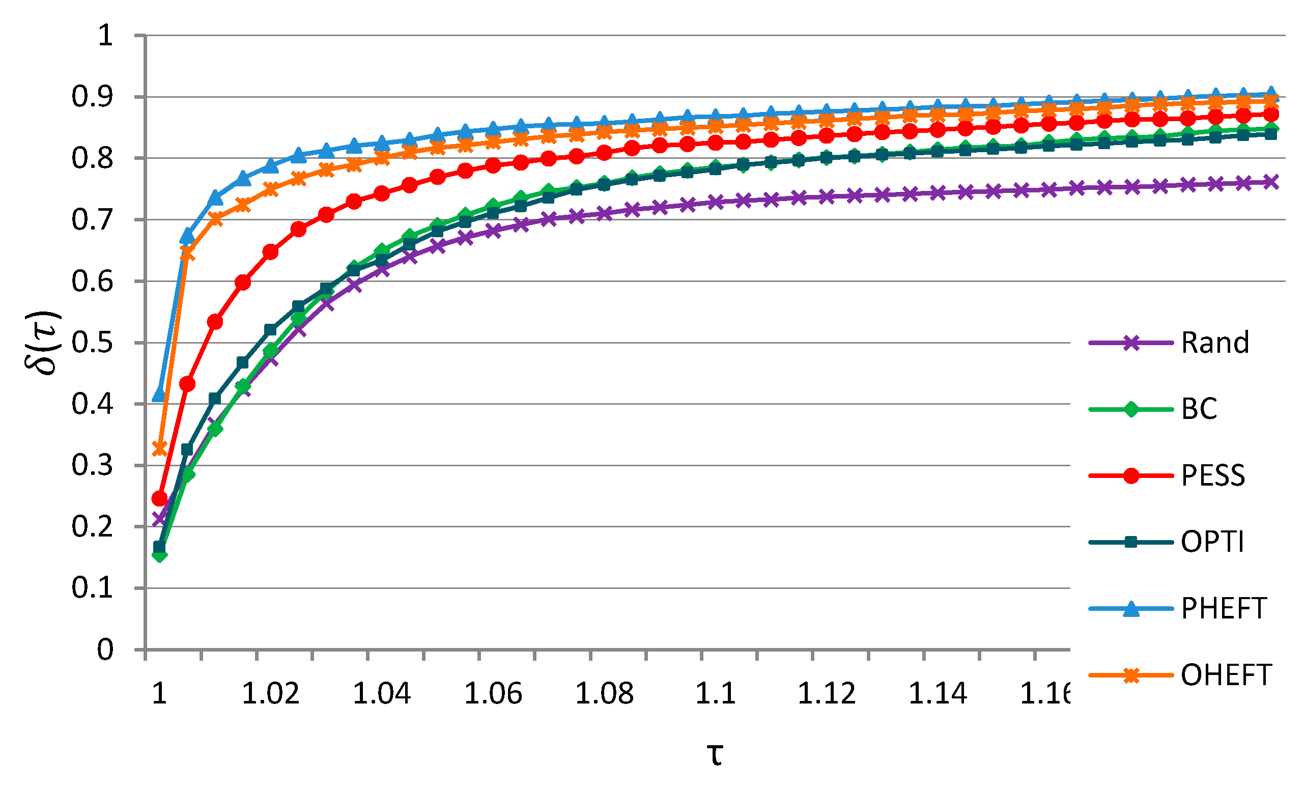
Figure 7 shows the mean performance profiles of all metrics, scenarios and test cases, considering . There were discrepancies in performance quality. If we want to obtain results within a factor of 1.02 of the best solution, then PHEFT generated them with probability 0.8, while Rand with a probability of 0.47. If we chose , then PHEFT produced results with a probability of 0.9, and Rand with a probability of 0.76.
7. Conclusions
Effective image and signal processing workflow management requires the efficient allocation of tasks to limited resources. In this paper, we presented allocation strategies that took into account both infrastructure information and workflow properties. We conducted a comprehensive performance evaluation study of six workflow scheduling strategies using simulation. We analyzed strategies that included task labeling, prioritization, resource selection, and DSP-cluster scheduling.
To provide effective guidance in choosing the best strategy, we performed a joint analysis of three metrics (makespan, mean critical path waiting time, and critical path slowdown) according to a degradation methodology and multi-criteria analysis, assuming the equal importance of each metric.
Our goal was to find a robust and well-performing strategy under all test cases, with the expectation that it would also perform well under other conditions, for example, with different cluster configurations and workloads.
Our study resulted in several contributions:
- (1)
- We examined overall DSP-cluster performance based on real image and signal processing data, considering Ligo and Montage applications;
- (2)
- We took into account communication latency, which is a major factor in DSP scheduling performance;
- (3)
- We showed that efficient job allocation depends not only on application properties and constraints but also on the nature of the infrastructure. To this end, we examined three configurations of DSP-clusters.
We found that an appropriate distribution of jobs over the clusters using a pessimistic approach had a higher performance than an allocation of jobs based on an optimistic one.
There were two differences to PHEFT strategy, compared to its original HEFT version. First, the data transfer cost within a workflow was set to maximal values for a given infrastructure to support pessimistic scenarios. All data transmissions were assumed to be made between different integrated modules and different DSPs to obtain the worst data transmission scenario with the maximal data rate coefficient.
Second, PHEFT had reduced time complexity compared to HEFT. It did not need to consider every combination of DSPs, where the two given tasks were executed, and did not need to take into account the data transfer rate between the two nodes to calculate a rank value (upward rank) based on mean computation and communication costs. Low complexity is important for industrial signal processing systems and real-time processing.
We conclude that for practical purposes, the scheduler PHEFT can improve the performance of workflow scheduling on DSP clusters. Although, more comprehensive algorithms can be adopted.
Author Contributions
All authors contributed to the analysis of the problem, designing algorithms, performing the experiments, analysis of data, and writing the paper.
Acknowledgments
This work was partially supported by RFBR, project No. 18-07-01224-a.
Conflicts of Interest
The authors declare no conflict of interest.
References
- Conway, R.W.; Maxwell, W.L.; Miller, L.W. Theory of Scheduling; Addison-Wesley: Reading, MA, USA, 1967. [Google Scholar]
- Błażewicz, J.; Ecker, K.H.; Pesch, E.; Schmidt, G.; Weglarz, J. Handbook on Scheduling: From Theory to Applications; Springer: Berlin, Germany, 2007. [Google Scholar]
- Myakochkin, Y. 32-bit superscalar DSP-processor with floating point arithmetic. Compon. Technol. 2013, 7, 98–100. [Google Scholar]
- TigerSHARC Embedded Processor ADSP-TS201S. Available online: http://www.analog.com/en/products/processors-dsp/dsp/tigersharc-processors/adsp-ts201s.html#product-overview (accessed on 15 May 2018).
- Muchnick, S.S. Advanced Compiler Design and Implementation; Morgan Kauffman: San Francisco, CA, USA, 1997. [Google Scholar]
- Novikov, S.V. Global Scheduling Methods for Architectures with Explicit Instruction Level Parallelism. Ph.D. Thesis, Institute of Microprocessor Computer Systems RAS (NIISI), Moscow, Russia, 2005. [Google Scholar]
- Wieczorek, M.; Prodan, R.; Fahringer, T. Scheduling of scientific workflows in the askalon grid environment. ACM Sigmod Rec. 2005, 34, 56–62. [Google Scholar] [CrossRef]
- Bittencourt, L.F.; Madeira, E.R.M. A dynamic approach for scheduling dependent tasks on the xavantes grid middleware. In Proceedings of the 4th International Workshop on Middleware for Grid Computing, Melbourne, Australia, 27 November–1 December 2006. [Google Scholar]
- Jia, Y.; Rajkumar, B. Scheduling scientific workflow applications with deadline and budget constraints using genetic algorithms. Sci. Program. 2006, 14, 217–230. [Google Scholar]
- Ramakrishnan, A.; Singh, G.; Zhao, H.; Deelman, E.; Sakellariou, R.; Vahi, K.; Blackburn, K.; Meyers, D.; Samidi, M. Scheduling data-intensive workflows onto storage-constrained distributed resources. In Proceedings of the 7th IEEE Symposium on Cluster Computing and the Grid, Rio De Janeiro, Brazil, 14–17 May 2007. [Google Scholar]
- Szepieniec, T.; Bubak, M. Investigation of the dag eligible jobs maximization algorithm in a grid. In Proceedings of the 2008 9th IEEE/ACM International Conference on Grid Computing, Tsukuba, Japan, 29 September–1 October 2008. [Google Scholar]
- Singh, G.; Su, M.-H.; Vahi, K.; Deelman, E.; Berriman, B.; Good, J.; Katz, D.S.; Mehta, G. Workflow task clustering for best effort systems with Pegasus. In Proceedings of the 15th ACM Mardi Gras conference, Baton Rouge, LA, USA, 29 January–3 February 2008. [Google Scholar]
- Singh, G.; Kesselman, C.; Deelman, E. Optimizing grid-based workflow execution. J. Grid Comput. 2005, 3, 201–219. [Google Scholar] [CrossRef]
- Tchernykh, A.; Lozano, L.; Schwiegelshohn, U.; Bouvry, P.; Pecero, J.-E.; Nesmachnow, S.; Drozdov, A. Online Bi-Objective Scheduling for IaaS Clouds with Ensuring Quality of Service. J. Grid Comput. 2016, 14, 5–22. [Google Scholar] [CrossRef]
- Tchernykh, A.; Ecker, K. Worst Case Behavior of List Algorithms for Dynamic Scheduling of Non-Unit Execution Time Tasks with Arbitrary Precedence Constrains. IEICE-Tran Fund Elec. Commun. Comput. Sci. 2008, 8, 2277–2280. [Google Scholar]
- Rodriguez, A.; Tchernykh, A.; Ecker, K. Algorithms for Dynamic Scheduling of Unit Execution Time Tasks. Eur. J. Oper. Res. 2003, 146, 403–416. [Google Scholar] [CrossRef]
- Tchernykh, A.; Trystram, D.; Brizuela, C.; Scherson, I. Idle Regulation in Non-Clairvoyant Scheduling of Parallel Jobs. Disc. Appl. Math. 2009, 157, 364–376. [Google Scholar] [CrossRef]
- Deelman, E.; Singh, G.; Su, M.H.; Blythe, J.; Gil, Y.; Kesselman, C.; Katz, D.S. Pegasus: A framework for mapping complex scientific workflows onto distributed systems. Sci. Program. 2005, 13, 219–237. [Google Scholar] [CrossRef]
- Blythe, J.; Jain, S.; Deelman, E.; Vahi, K.; Gil, Y.; Mandal, A.; Kennedy, K. Task Scheduling Strategies for Workflow-based Applications in Grids. In Proceedings of the IEEE International Symposium on Cluster Computing and the Grid, Cardiff, Wales, UK, 9–12 May 2005. [Google Scholar]
- Kliazovich, D.; Pecero, J.; Tchernykh, A.; Bouvry, P.; Khan, S.; Zomaya, A. CA-DAG: Modeling Communication-Aware Applications for Scheduling in Cloud Computing. J. Grid Comput. 2016, 14, 23–39. [Google Scholar] [CrossRef]
- Bittencourt, L.F.; Madeira, E.R.M. Towards the scheduling of multiple workflows on computational grids. J. Grid Comput. 2010, 8, 419–441. [Google Scholar] [CrossRef]
- Zhao, H.; Sakellariou, R. Scheduling multiple dags onto heterogeneous systems. In Proceedings of the 20th International Parallel and Distributed Processing Symposium, Rhodes Island, Greece, 25–29 April 2006. [Google Scholar]
- Topcuouglu, H.; Hariri, S.; Wu, M.-Y. Performance-effective and low-complexity task scheduling for heterogeneous computing. IEEE Trans. Parallel Distrib. Syst. 2002, 13, 260–274. [Google Scholar] [CrossRef]
- Sakellariou, R.; Zhao, H. A hybrid heuristic for dag scheduling on heterogeneous systems. In Proceedings of the 13th IEEE Heterogeneous Computing Workshop, Santa Fe, NM, USA, 26 April 2004. [Google Scholar]
- Bittencourt, L.F.; Sakellariou, R.; Madeira, E.R. DAG Scheduling Using a Lookahead Variant of the Heterogeneous Earliest Finish Time Algorithm. In Proceedings of the 18th Euromicro Conference on Parallel, Distributed and Network-Based Processing, Pisa, Italy, 17–19 February 2010. [Google Scholar]
- Zhao, H.; Sakellariou, R. An Experimental Investigation into the Rank Function of the Heterogeneous Earliest Finish Time Scheduling Algorithm; Springer: Berlin/Heidelberg, Germany, 2003. [Google Scholar]
- Pegasus. Available online: http://pegasus.isi.edu/workflow_gallery/index.php (accessed on 15 May 2018).
- Hirales-Carbajal, A.; Tchernykh, A.; Roblitz, T.; Yahyapour, R. A grid simulation framework to study advance scheduling strategies for complex workflow applications. In Proceedings of the 2010 IEEE International Symposium on Parallel & Distributed Processing, Workshops and Phd Forum (IPDPSW), Atlanta, GA, USA, 19–23 April 2010. [Google Scholar]
- Hirales-Carbajal, A.; Tchernykh, A.; Yahyapour, R.; Röblitz, T.; Ramírez-Alcaraz, J.-M.; González-García, J.-L. Multiple Workflow Scheduling Strategies with User Run Time Estimates on a Grid. J. Grid Comput. 2012, 10, 325–346. [Google Scholar] [CrossRef]
- Ramírez-Velarde, R.; Tchernykh, A.; Barba-Jimenez, C.; Hirales-Carbajal, A.; Nolazco, J. Adaptive Resource Allocation in Computational Grids with Runtime Uncertainty. J. Grid Comput. 2017, 15, 415–434. [Google Scholar] [CrossRef]
- Tchernykh, A.; Schwiegelsohn, U.; Talbi, E.-G.; Babenko, M. Towards understanding uncertainty in cloud computing with risks of confidentiality, integrity, and availability. J. Comput. Sci. 2016. [Google Scholar] [CrossRef]
- Tchernykh, A.; Schwiegelsohn, U.; Alexandrov, V.; Talbi, E.-G. Towards Understanding Uncertainty in Cloud Computing Resource Provisioning. Proced. Comput. Sci. 2015, 51, 1772–1781. [Google Scholar] [CrossRef] [Green Version]
- Dolan, E.D.; Moré, J.J.; Munson, T.S. Optimality measures for performance profiles. Siam. J. Optim. 2006, 16, 891–909. [Google Scholar] [CrossRef]
Figure 1.
Digital signal processor (DSP) cluster.
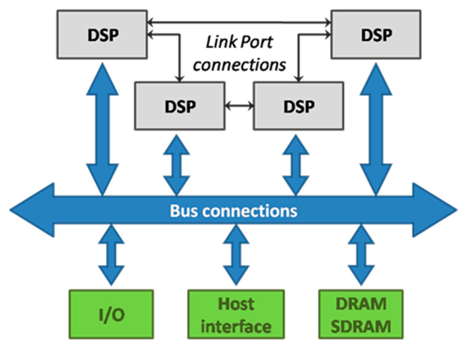
Figure 2.
Examples of communication topology of DSP-processors: (a) uni-directional; (b) bi-directional; (c) all to all.
Figure 2.
Examples of communication topology of DSP-processors: (a) uni-directional; (b) bi-directional; (c) all to all.
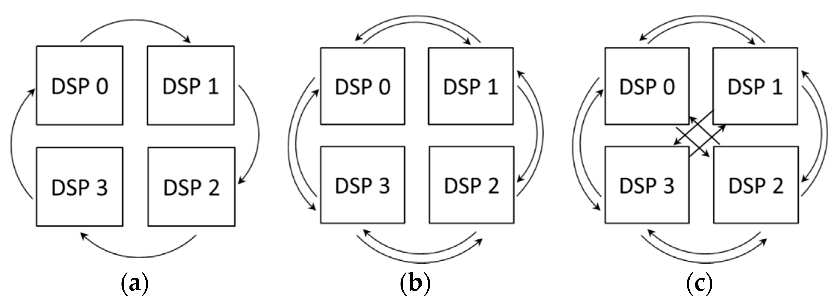
Figure 3.
DSP cluster configuration. (a) Cluster A; (b) Cluster B.

Figure 4.
Performance degradation.
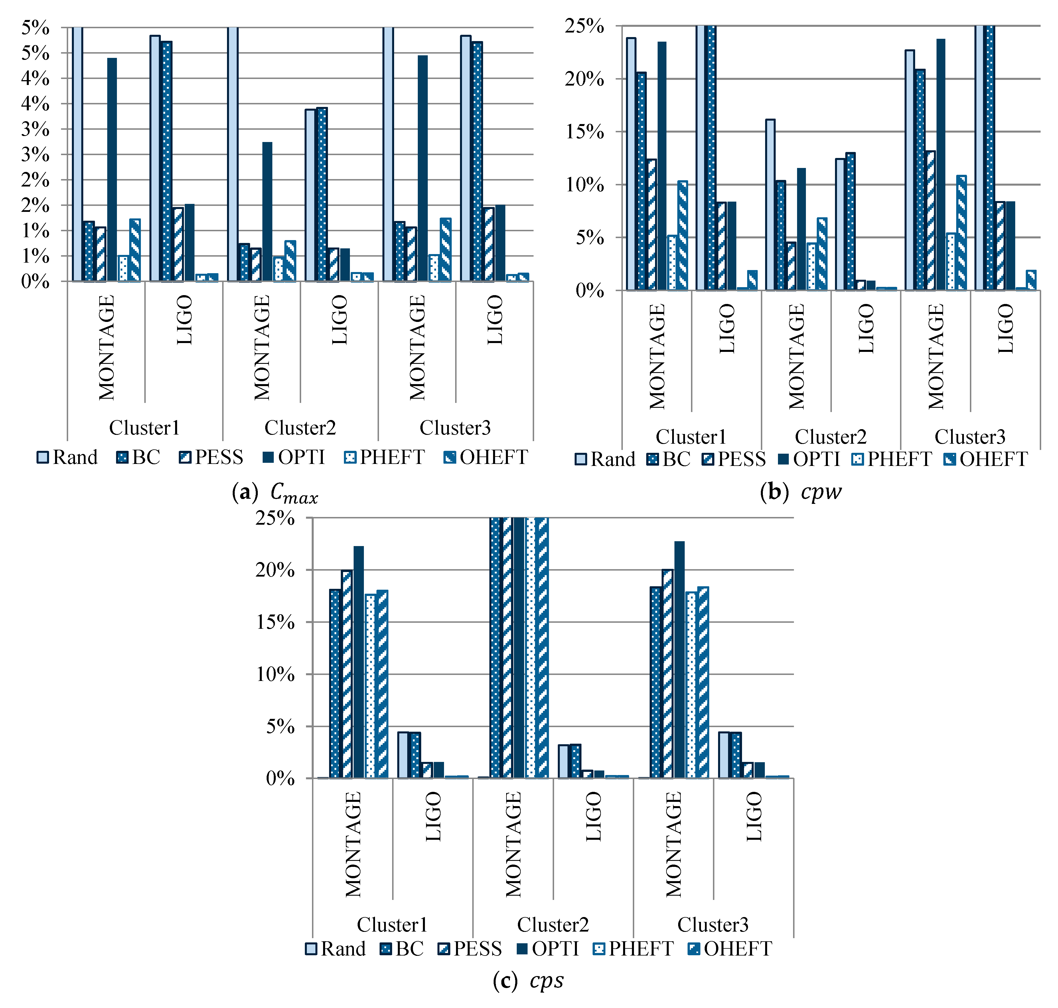
Figure 5.
performance profile, . (a) Montage; (b) Ligo.
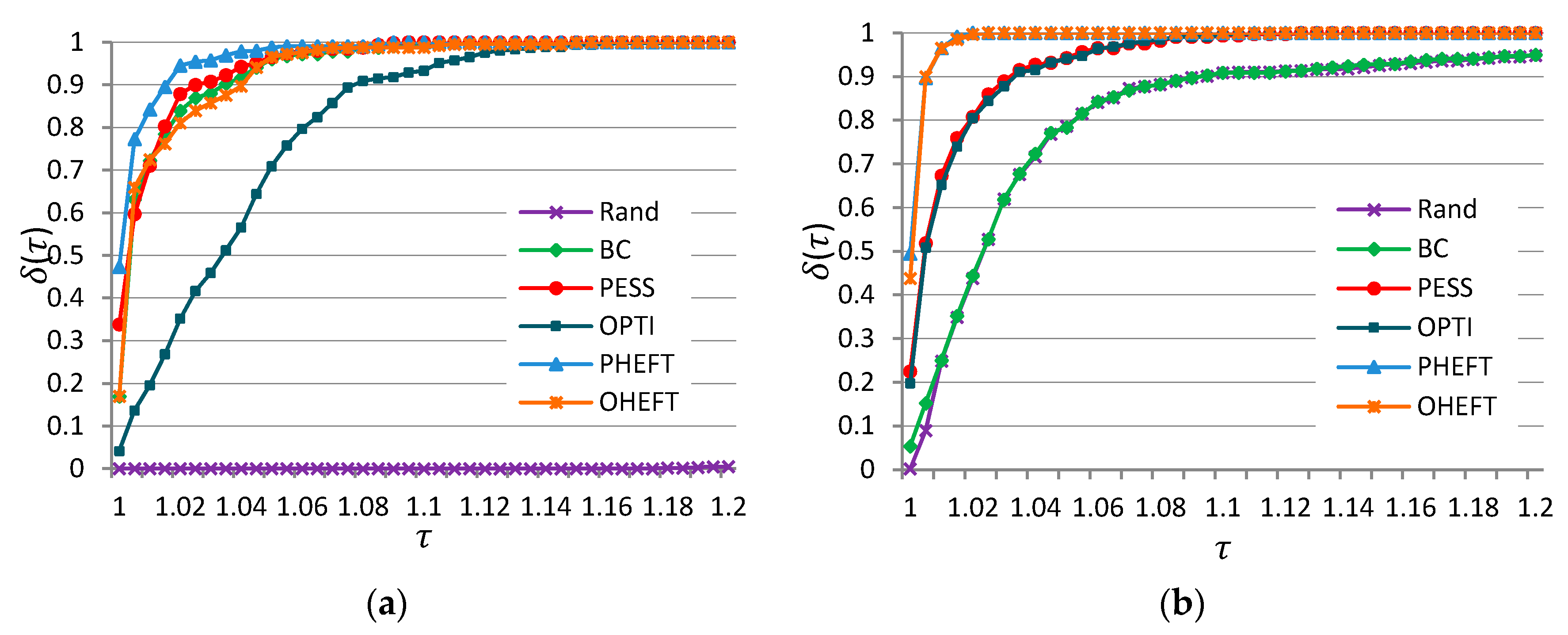
Figure 6.
performance profile, . (a) Montage; (b) Ligo.
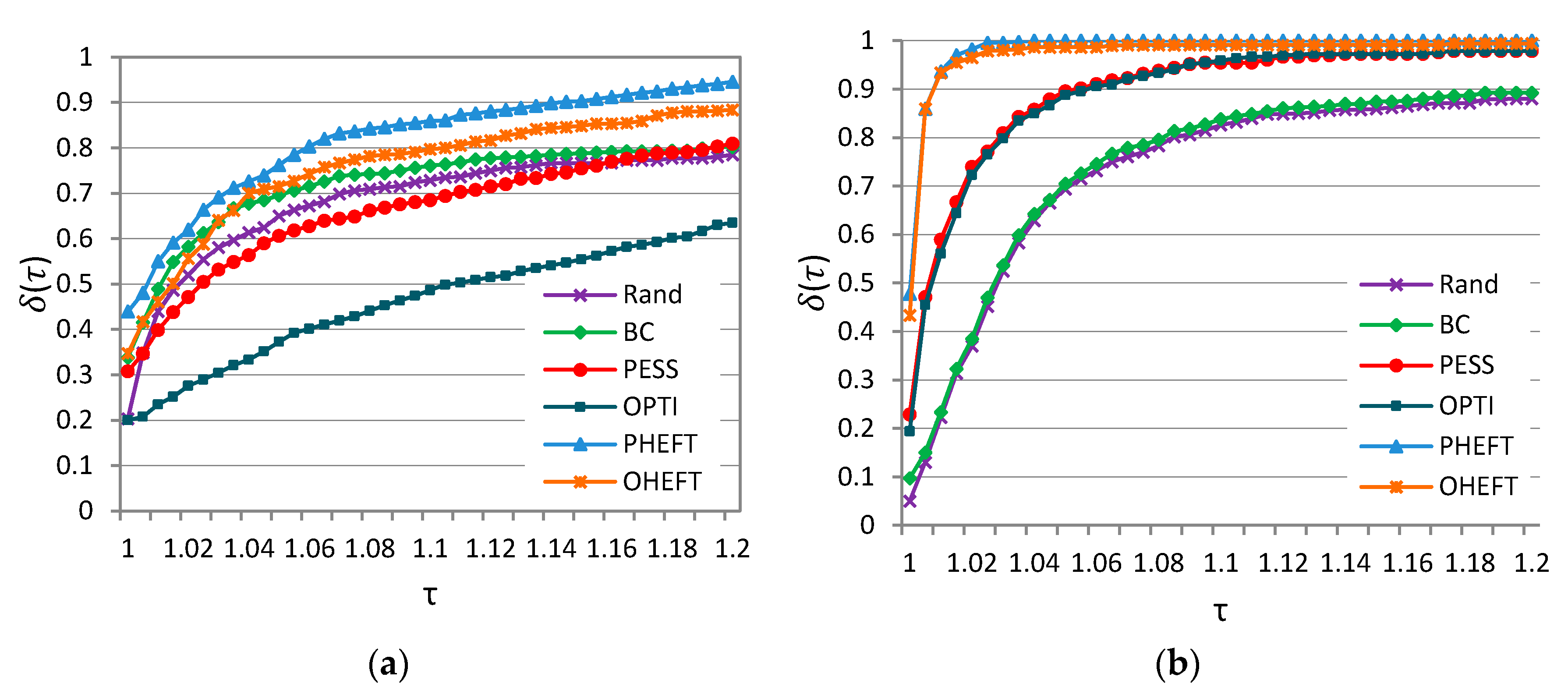
Figure 7.
Mean performance profile over all metrics and test cases, .

Table 1.
Data rate coefficients of the cluster of DSP with four integrated modules (IMs).
| IM | 1 | 2 | 3 | 4 |
|---|---|---|---|---|
| 1 | ε | |||
| 2 | ε | |||
| 3 | ε | |||
| 4 | ε |
Table 2.
Data rate coefficient matrix D for three communication topologies between DSP-processors.
| (a) Uni-Directional | (b) Bi-Directional | (c) All to All | |||||||||
|---|---|---|---|---|---|---|---|---|---|---|---|
| 0 | 1 | 2 | 3 | 0 | 1 | 2 | 1 | 0 | 1 | 1 | 1 |
| 3 | 0 | 1 | 2 | 1 | 0 | 1 | 2 | 1 | 0 | 1 | 1 |
| 2 | 3 | 0 | 1 | 2 | 1 | 0 | 1 | 1 | 1 | 0 | 1 |
| 1 | 2 | 3 | 0 | 1 | 2 | 1 | 0 | 1 | 1 | 1 | 0 |
Table 3.
Task allocation strategies.
| Description | |
|---|---|
| Rand | Allocates task to a DSP with the number randomly generated from a uniform distribution in the range [1,m] |
| BC (best core) | Allocates task to the DSP that can start the task as early as possible considering communication delay of all input data |
| PESS (pessimistic) | Allocates task from the ordered list to the DSP according to Worst Downward Rank (WDR). |
| OPTI (optimistic) | Allocates task from the ordered list to the DSP according to Best Downward Rank (BDR). |
| PHEFT (pessimistic HEFT) | Allocates task from the ordered list to the DSP according to Worst Upward Rank (WUR) |
| OHEFT (optimistic HEFT) | Allocates task from the ordered list to the DSP according to Best Upward Rank (BUR) |
Table 4.
Experimental settings.
| Description | Settings |
|---|---|
| Workload type | 220 Montage workflows, 98 Ligo workflows |
| DSP clusters | 3 |
| Cluster 1 | 5 in a cluster B, 4 DSP per module |
| Cluster 2 | 2 in a cluster A, 4 DSP per module |
| Cluster 3 | 5 in a cluster A, 4 DSP per module |
| Data transmission coefficient K | 0—within the same DSP |
| 1—between connected DSPs in a ; | |
| 20—between DSP of different | |
| Metrics | , , |
| Number of experiments | 318 |
Table 5.
Rounded performance degradation and ranking.
| Criteria | Strategy | ||||||
|---|---|---|---|---|---|---|---|
| Rand | BC | PESS | OPTI | PHEFT | OHEFT | ||
| Montage | 3.189 | 0.010 | 0.009 | 0.039 | 0.005 | 0.011 | |
| 0.209 | 0.173 | 0.100 | 0.196 | 0.050 | 0.093 | ||
| 0.001 | 0.305 | 0.320 | 0.348 | 0.302 | 0.306 | ||
| Mean | 1.133 | 0.163 | 0.143 | 0.194 | 0.119 | 0.137 | |
| Rank | 6 | 4 | 3 | 5 | 1 | 2 | |
| Ligo | 0.044 | 0.043 | 0.012 | 0.012 | 0.001 | 0.002 | |
| 0.580 | 0.542 | 0.059 | 0.059 | 0.002 | 0.013 | ||
| 0.040 | 0.040 | 0.012 | 0.013 | 0.002 | 0.002 | ||
| Mean | 0.221 | 0.208 | 0.028 | 0.028 | 0.002 | 0.005 | |
| Rank | 6 | 5 | 3 | 4 | 1 | 2 | |
| All test cases | 1.616 | 0.027 | 0.011 | 0.025 | 0.003 | 0.006 | |
| 0.394 | 0.357 | 0.079 | 0.128 | 0.026 | 0.053 | ||
| 0.020 | 0.173 | 0.166 | 0.180 | 0.152 | 0.154 | ||
| Mean | 0.677 | 0.186 | 0.085 | 0.111 | 0.060 | 0.071 | |
| Rank | 6 | 5 | 3 | 4 | 1 | 2 | |
© 2018 by the authors. Licensee MDPI, Basel, Switzerland. This article is an open access article distributed under the terms and conditions of the Creative Commons Attribution (CC BY) license (http://creativecommons.org/licenses/by/4.0/).
Share and Cite
MDPI and ACS Style
Drozdov, A.Y.; Tchernykh, A.; Novikov, S.V.; Vladislavlev, V.E.; Rivera-Rodriguez, R. PHEFT: Pessimistic Image Processing Workflow Scheduling for DSP Clusters. Algorithms 2018, 11, 76. https://doi.org/10.3390/a11050076
AMA Style
Drozdov AY, Tchernykh A, Novikov SV, Vladislavlev VE, Rivera-Rodriguez R. PHEFT: Pessimistic Image Processing Workflow Scheduling for DSP Clusters. Algorithms. 2018; 11(5):76. https://doi.org/10.3390/a11050076
Chicago/Turabian StyleDrozdov, Alexander Yu., Andrei Tchernykh, Sergey V. Novikov, Victor E. Vladislavlev, and Raul Rivera-Rodriguez. 2018. "PHEFT: Pessimistic Image Processing Workflow Scheduling for DSP Clusters" Algorithms 11, no. 5: 76. https://doi.org/10.3390/a11050076
Note that from the first issue of 2016, this journal uses article numbers instead of page numbers. See further details here.