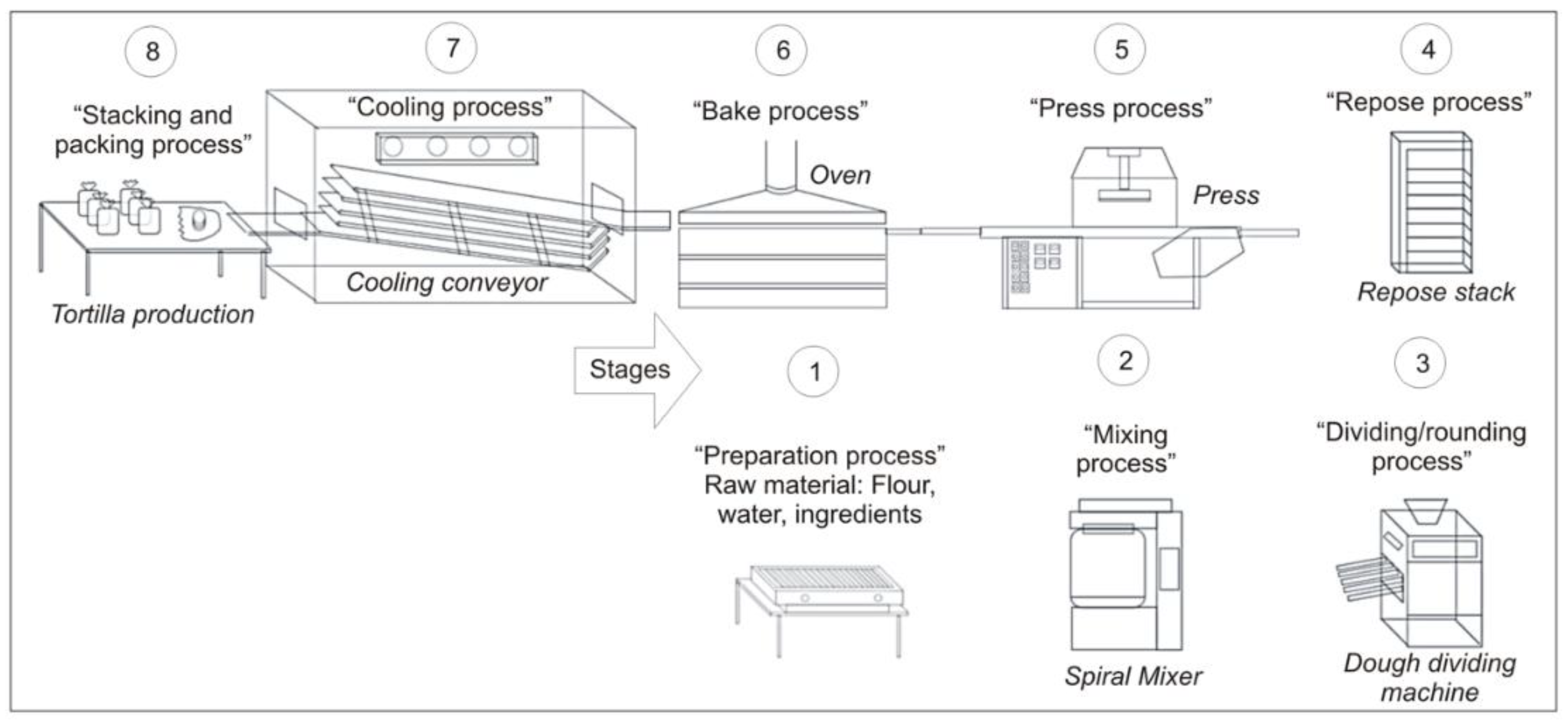
Figure 1.
Tortilla production line.
Figure 1.
Tortilla production line.
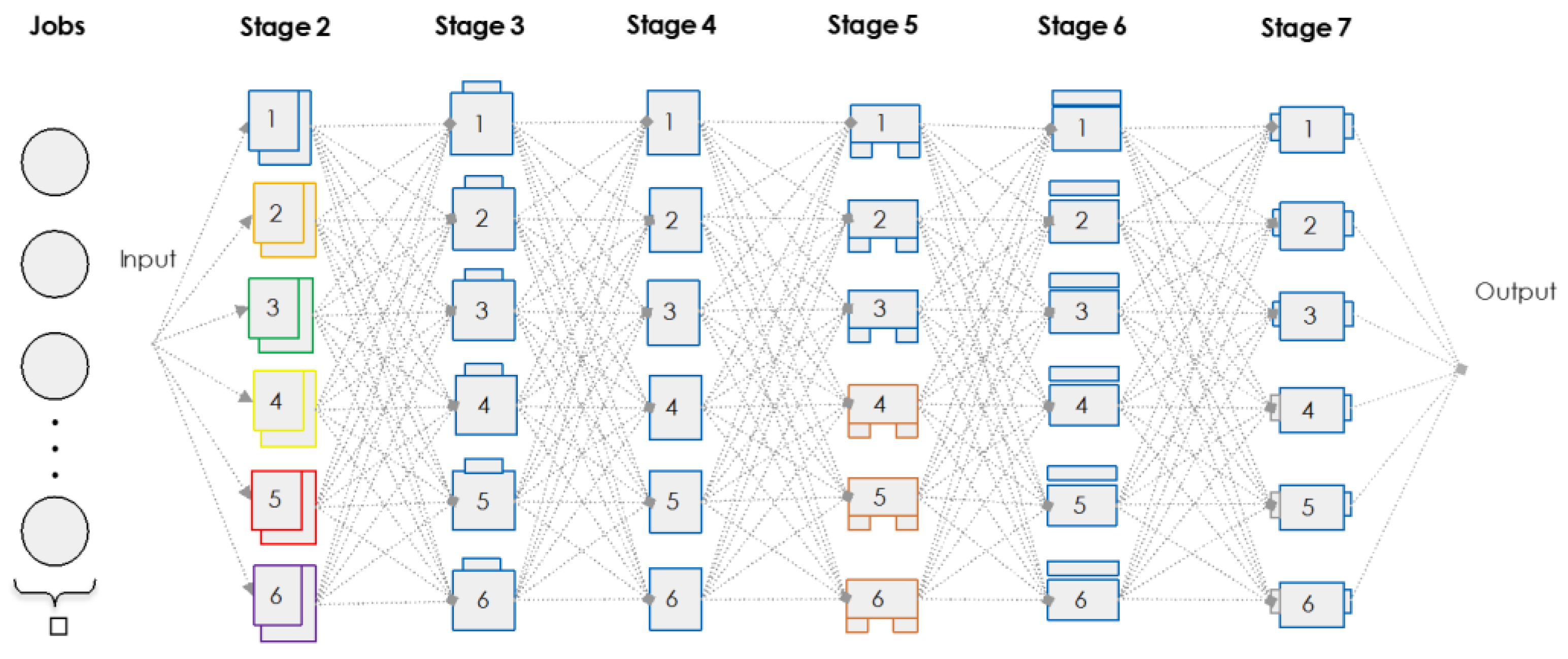
Figure 2.
Six-stage hybrid flow shop.
Figure 2.
Six-stage hybrid flow shop.
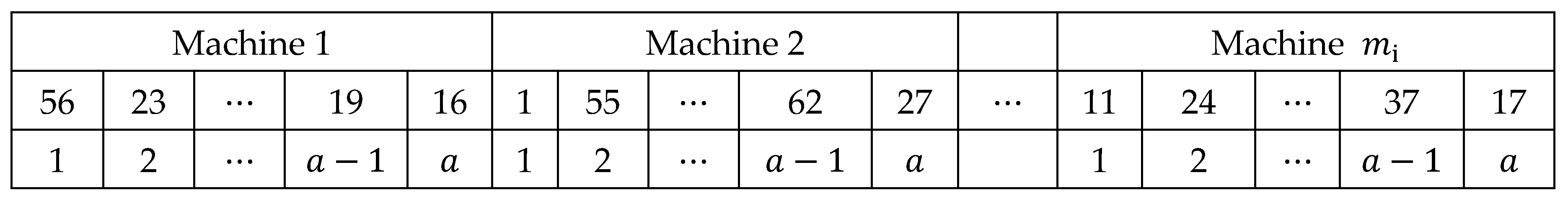
Figure 3.
Example of the representation of the chromosome for machines per stage.
Figure 3.
Example of the representation of the chromosome for machines per stage.
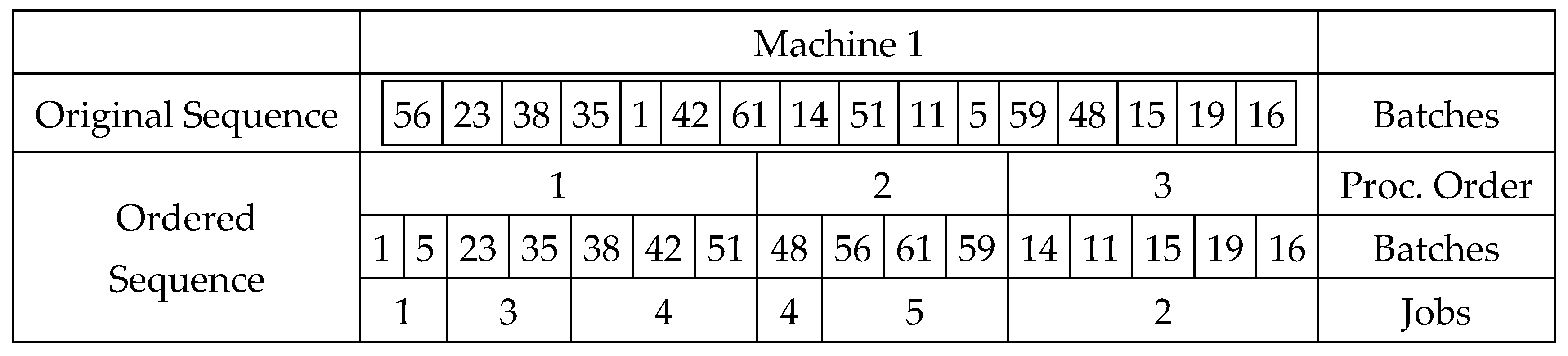
Figure 4.
Example of tasks on Machine 1.
Figure 4.
Example of tasks on Machine 1.
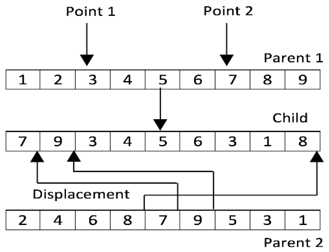
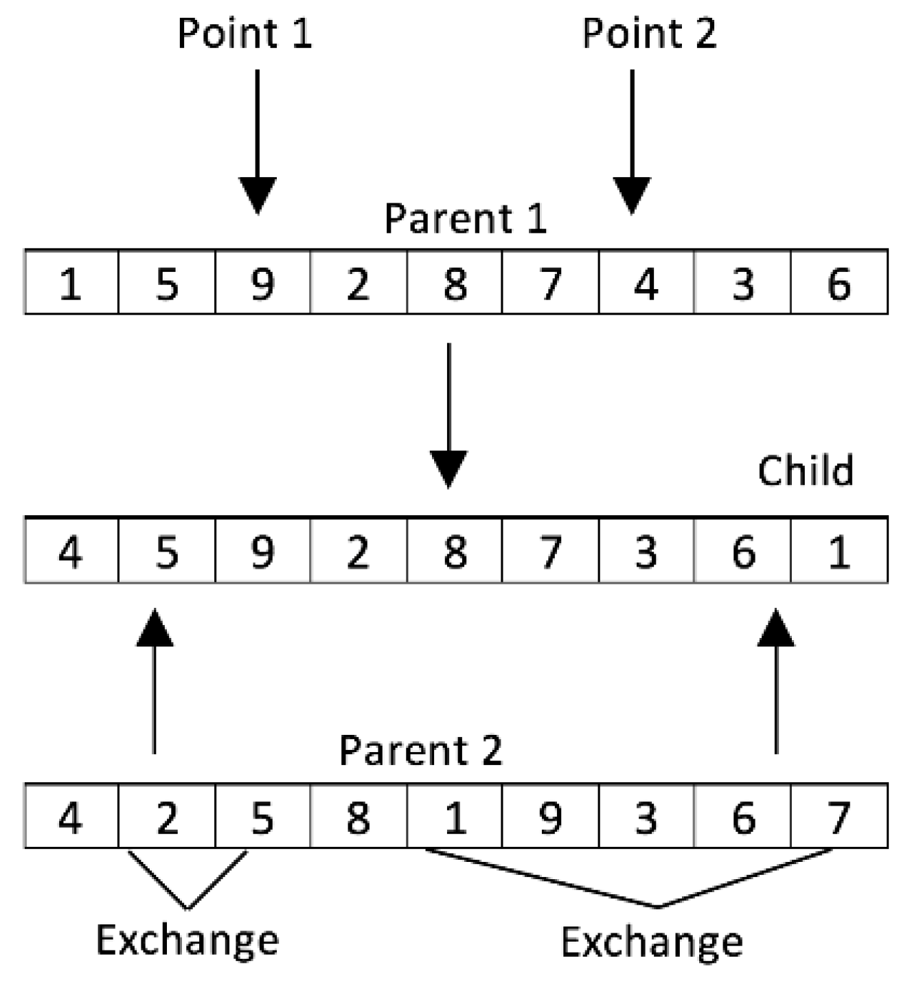
Figure 5.
Partially mapped crossover (PMX) operator.
Figure 5.
Partially mapped crossover (PMX) operator.
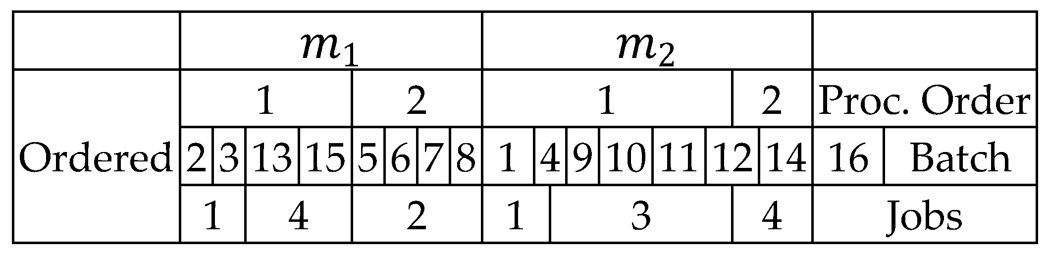
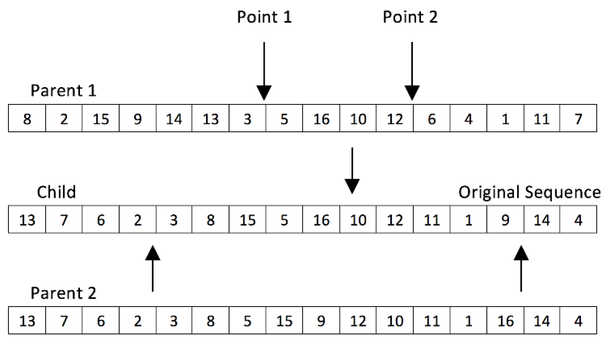
Figure 6.
PMX crossover operator example with batch index.
Figure 6.
PMX crossover operator example with batch index.
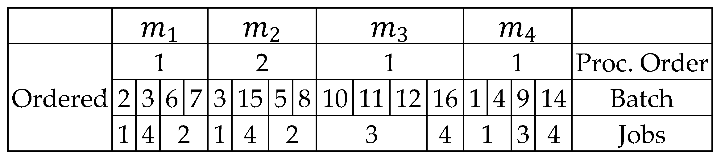
Figure 7.
Chromosome representation example with two machines per stage.
Figure 7.
Chromosome representation example with two machines per stage.
Figure 8.
Chromosome representation example with four machines per stage.
Figure 8.
Chromosome representation example with four machines per stage.
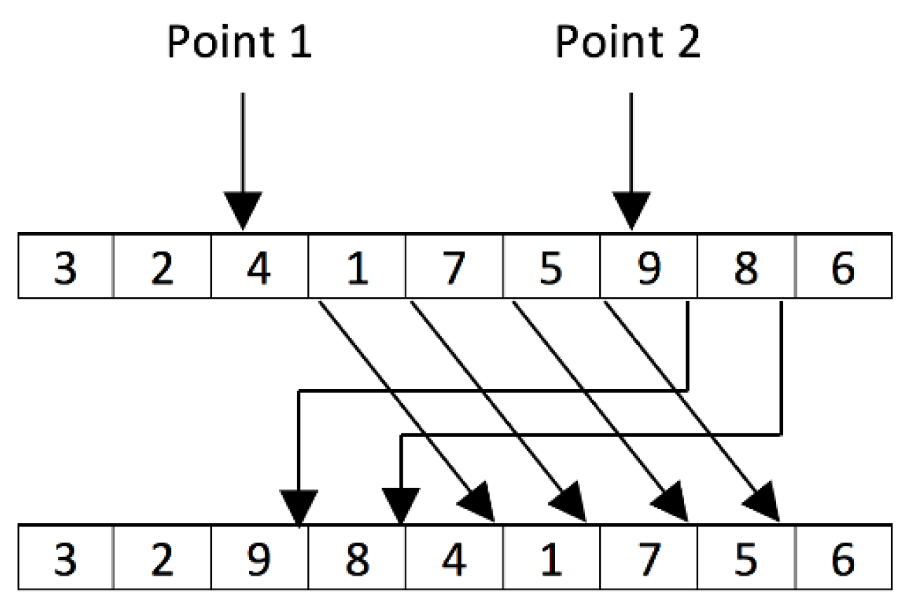
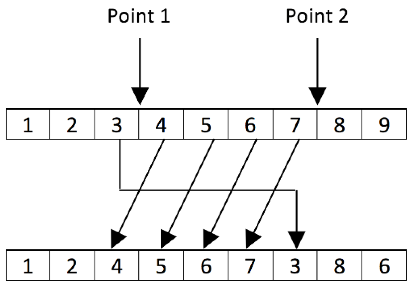
Figure 9.
Order crossover (OX) operator.
Figure 9.
Order crossover (OX) operator.
Figure 10.
Displacement mutation operator.
Figure 10.
Displacement mutation operator.
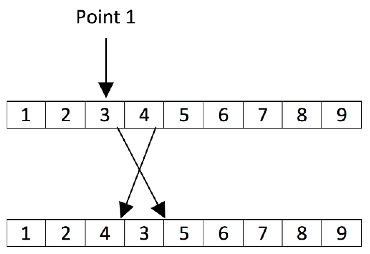
Figure 11.
Exchange mutation operator.
Figure 11.
Exchange mutation operator.
Figure 12.
Insertion mutation operator.
Figure 12.
Insertion mutation operator.
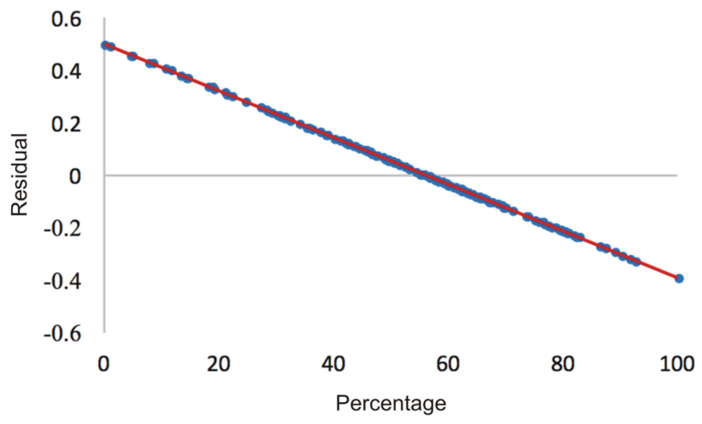
Figure 13.
Graph of the normal probability of waste for six machines per stage.
Figure 13.
Graph of the normal probability of waste for six machines per stage.
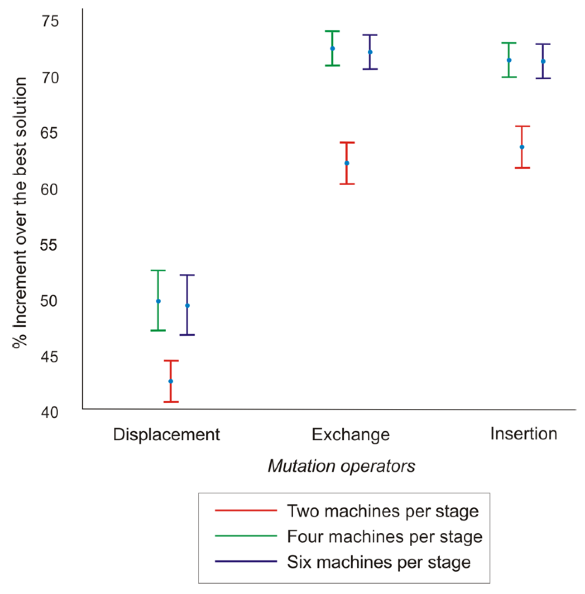
Figure 14.
Means and 95% LSD confidence intervals of mutation operators.
Figure 14.
Means and 95% LSD confidence intervals of mutation operators.
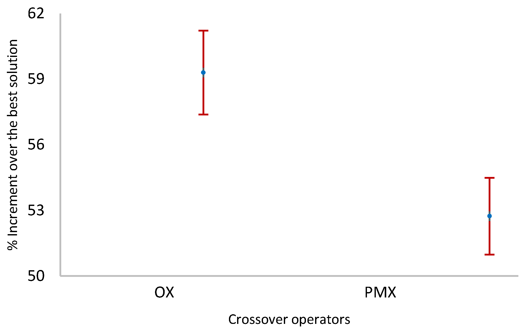
Figure 15.
Means and 95% LSD confidence intervals of crossover operators—two machines per stage.
Figure 15.
Means and 95% LSD confidence intervals of crossover operators—two machines per stage.
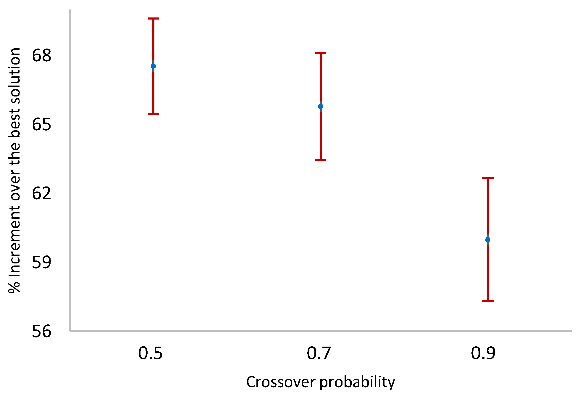
Figure 16.
Means and 95% LSD confidence intervals of crossover probability—four machines per stage.
Figure 16.
Means and 95% LSD confidence intervals of crossover probability—four machines per stage.
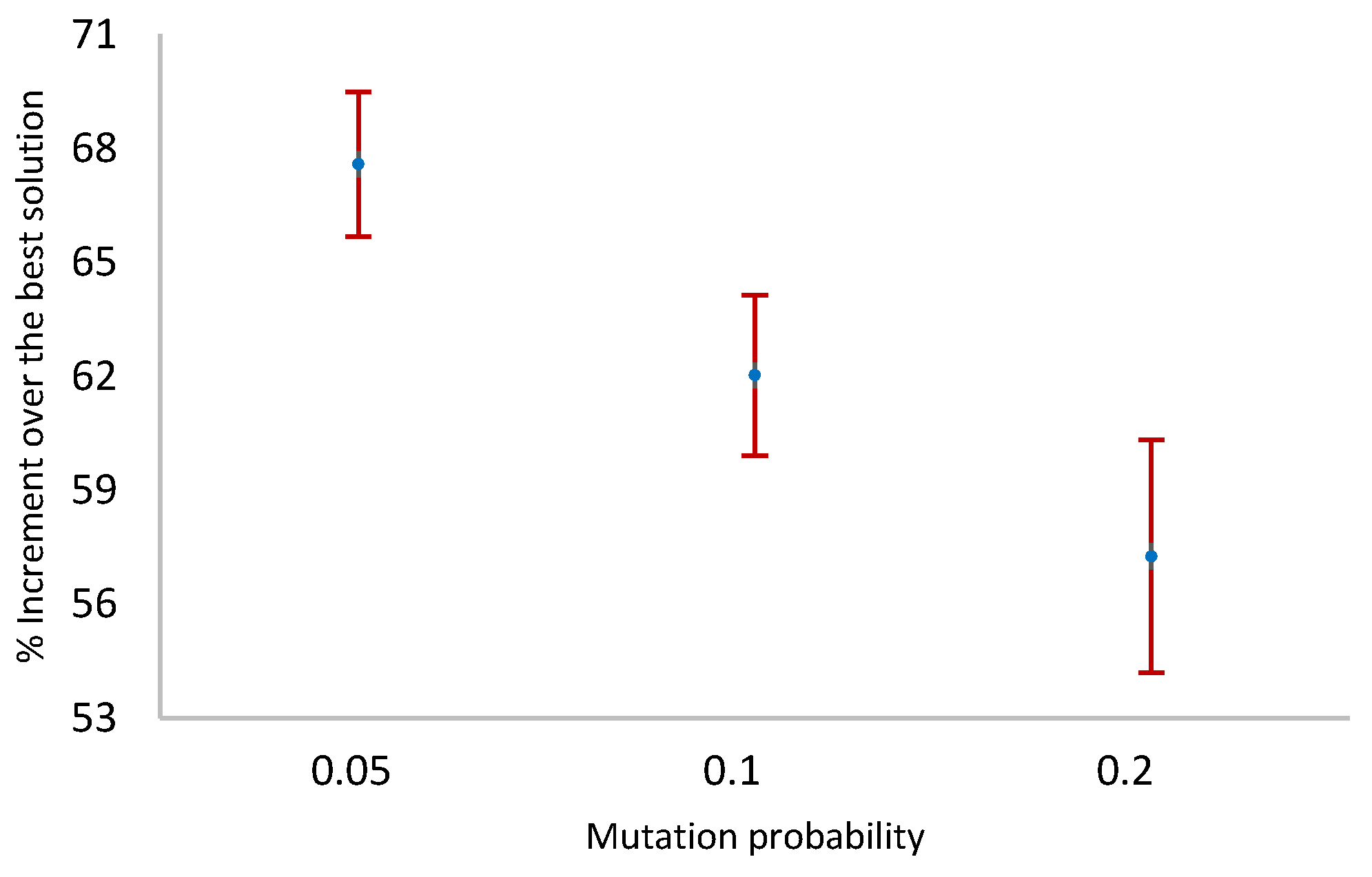
Figure 17.
Means and 95% LSD confidence intervals of mutation probability—six machines per stage.
Figure 17.
Means and 95% LSD confidence intervals of mutation probability—six machines per stage.
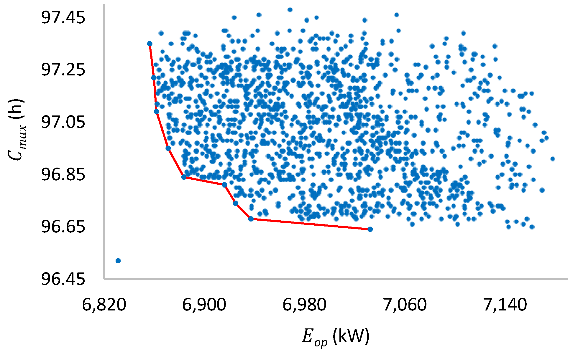
Figure 18.
Pareto front for two machines per stage.
Figure 18.
Pareto front for two machines per stage.
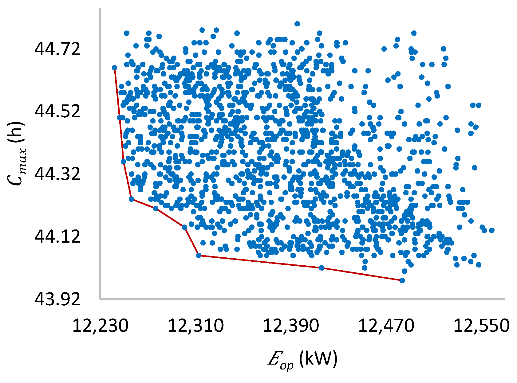
Figure 19.
Pareto front for four machines per stage.
Figure 19.
Pareto front for four machines per stage.
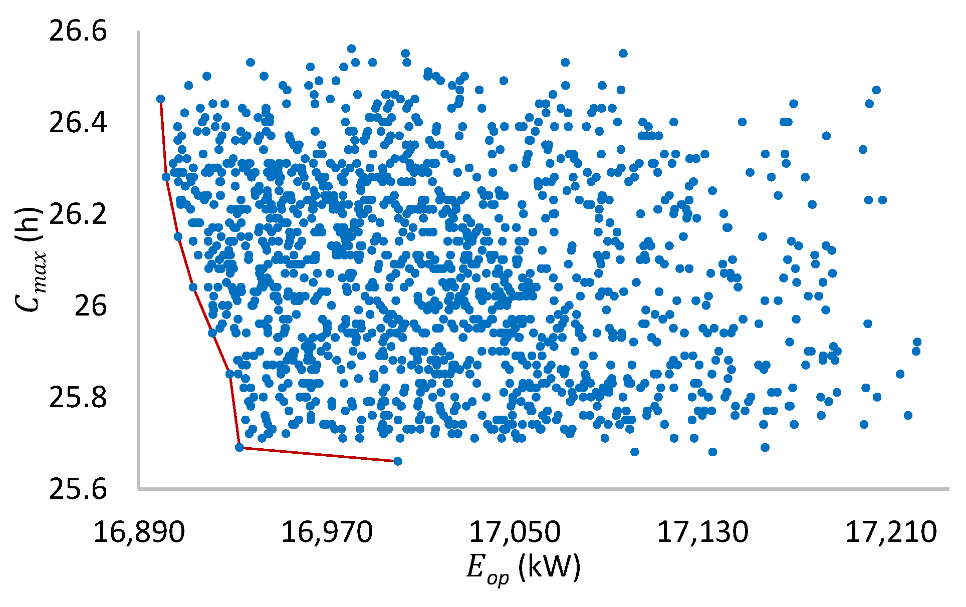
Figure 20.
Pareto front for six machines per stage.
Figure 20.
Pareto front for six machines per stage.
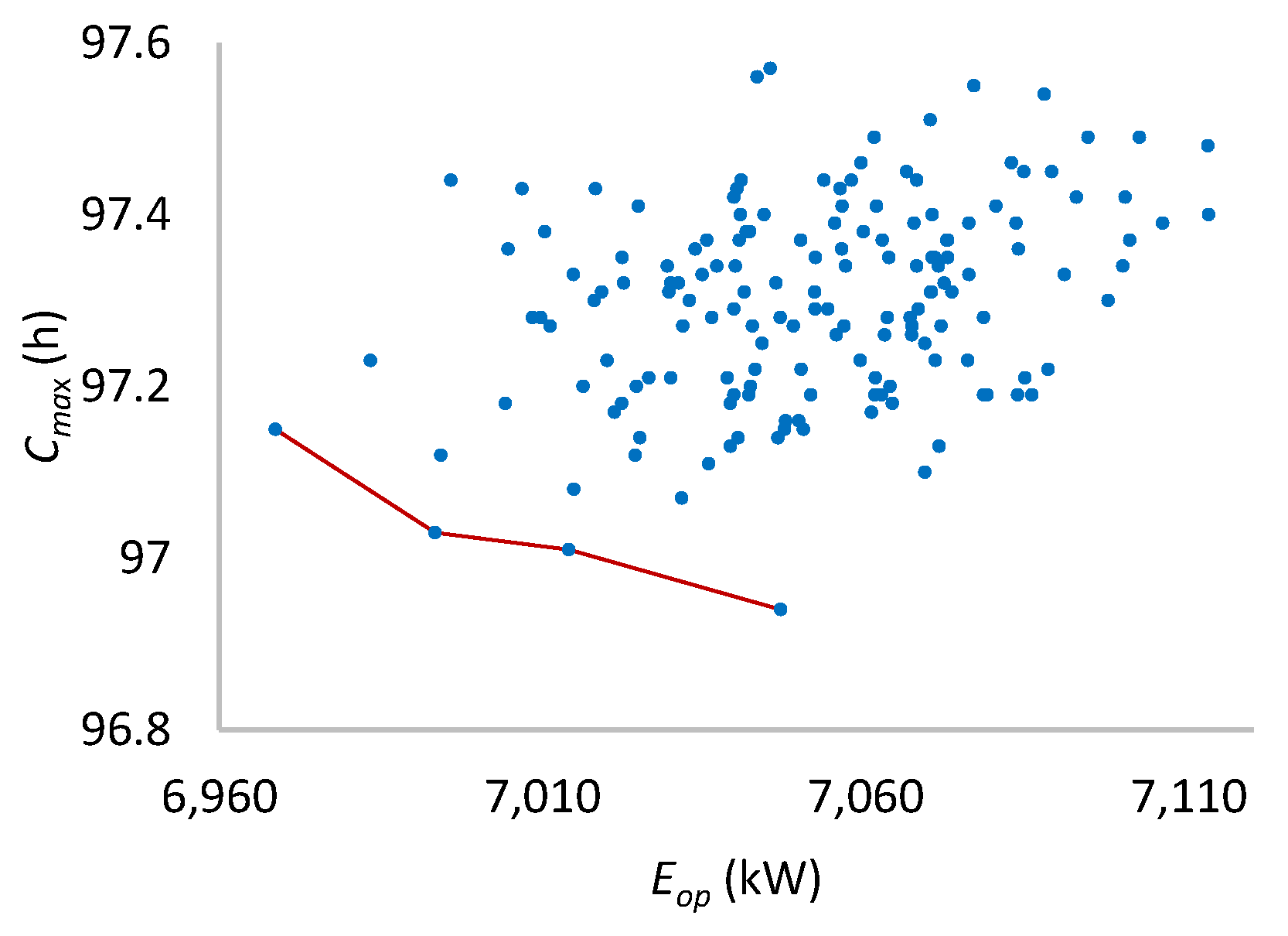
Figure 21.
Pareto front for two machines per stage.
Figure 21.
Pareto front for two machines per stage.
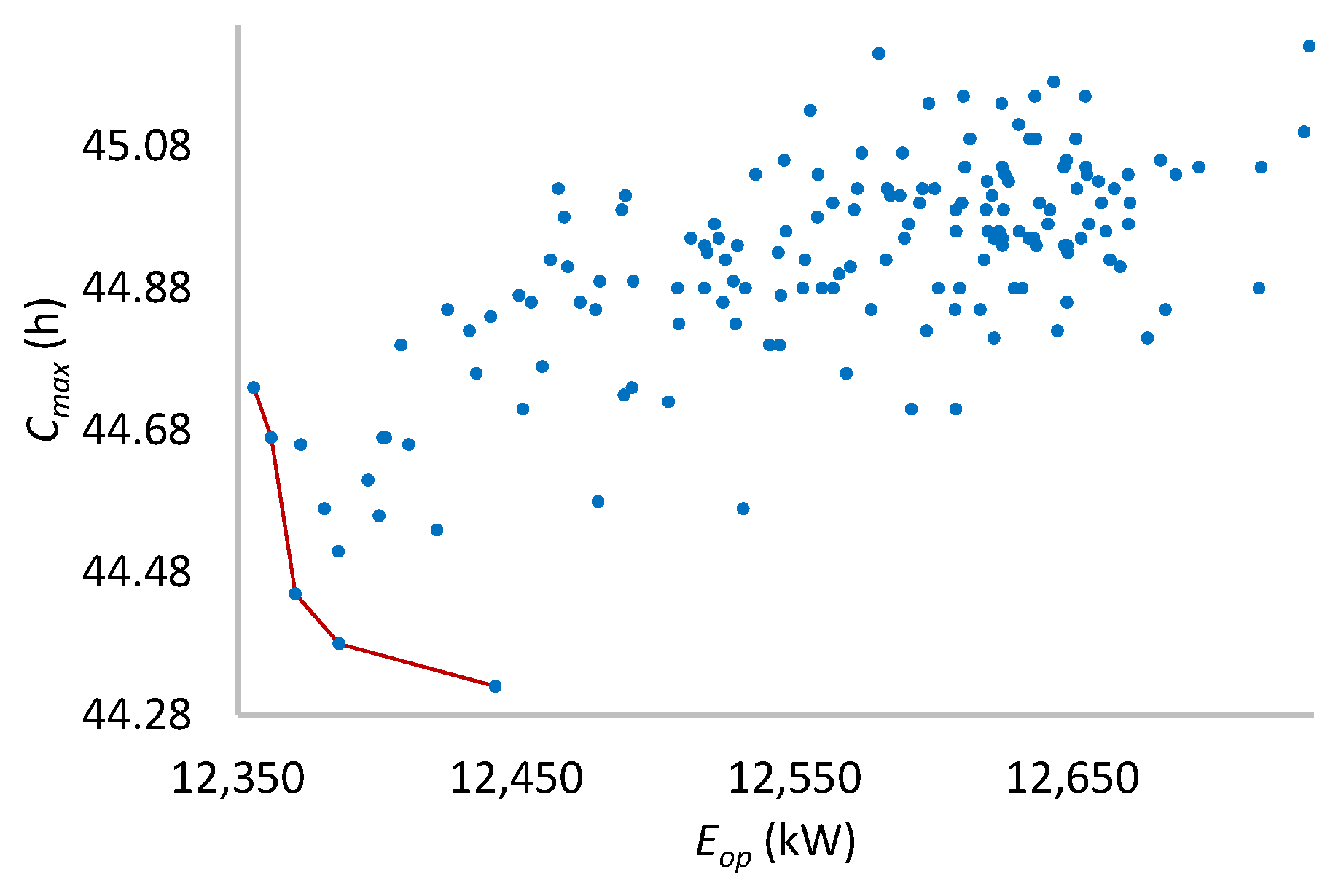
Figure 22.
Pareto front for four machines per stage.
Figure 22.
Pareto front for four machines per stage.
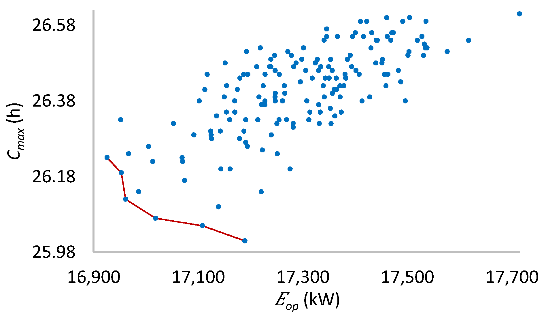
Figure 23.
Pareto front for six machines per stage.
Figure 23.
Pareto front for six machines per stage.
Figure 24.
of B&B algorithm and industry.
Figure 24.
of B&B algorithm and industry.
Figure 25.
Eop of B&B algorithm and industry.
Figure 25.
Eop of B&B algorithm and industry.
Table 1.
The processing capacity of machines in Stage 2 (kg per minute).
Table 1.
The processing capacity of machines in Stage 2 (kg per minute).
| Stage | 2 |
|---|
| Machines | 1 | 2 | 3 | 4 | 5 | 6 |
|---|
| Jobs 1–5 | 80 | 80 | 100 | 130 | 160 | 200 |
Table 2.
The processing capacity of machines in Stages 3–7 (kg per minute).
Table 2.
The processing capacity of machines in Stages 3–7 (kg per minute).
| Stage | 3 | 4 | 5 | 6 | 7 |
|---|
| Machines | 1–6 | 1–6 | 1–3 | 4–6 | 1–6 | 1–6 |
|---|
| Jobs | 1 | 1.3 | 200 | 7.2 | 9.6 | 9.6 | 9.6 |
| 2 | 1.3 | 200 | 6.4 | 8.8 | 8.8 | 8.8 |
| 3 | 0.44 | 200 | 2.4 | 4 | 4 | 4 |
| 4 | 0.31 | 200 | 3.2 | 4.8 | 4.8 | 4.8 |
| 5 | 1.3 | 200 | 4 | 8.8 | 8.8 | 8.8 |
Table 3.
Energy consumption of machines (kW per minute).
Table 3.
Energy consumption of machines (kW per minute).
| Stage | 2 | 3 | 4 | 5 | 6 | 7 |
|---|
| Machine | 1 | 0.09 | 0.03 | 0 | 0.62 | 0.04 | 0.12 |
| 2 | 0.09 | 0.03 | 0 | 0.62 | 0.04 | 0.12 |
| 3 | 0.11 | 0.03 | 0 | 0.62 | 0.04 | 0.12 |
| 4 | 0.14 | 0.03 | 0 | 0.9 | 0.04 | 0.12 |
| 5 | 0.23 | 0.03 | 0 | 0.9 | 0.04 | 0.12 |
| 6 | 0.23 | 0.03 | 0 | 0.9 | 0.04 | 0.12 |
Table 4.
Job characteristics.
Table 4.
Job characteristics.
| Job j | Name | Type | Group | Batch Limits |
|---|
| 1 | Regular | 1 | 1 | 356–446 |
| 2 | Integral | 2 | 2 | 34–61 |
| 3 | Class 18 pcs | 3 | 1 | 7–10 |
| 4 | Taco 50 | 4 | 1 | 13–22 |
| 5 | MegaBurro | 5 | 1 | 12–20 |
Table 5.
Processing time of job at machine in stage for each 10 kg.
Table 5.
Processing time of job at machine in stage for each 10 kg.
| Stage | 2 | 3 | 4 | 5 | 6 | 7 |
|---|
| Machines | 1–6 | 1–6 | 1–6 | 1–3 | 4–6 | 1–6 | 1–6 |
|---|
| Jobs | 1 | 1 | 1.25 | 45 | 1.43 | 1.07 | 12.15 | 17.25 |
| 2 | 1 | 1.25 | 45 | 1.48 | 1.11 | 12.15 | 17.25 |
| 3 | 1 | 4.38 | 45 | 3.69 | 2.77 | 21.38 | 26.48 |
| 4 | 1 | 3.13 | 45 | 3.00 | 2.25 | 24.50 | 29.60 |
| 5 | 1 | 0.42 | 45 | 2.28 | 1.14 | 18.24 | 23.34 |
Table 6.
Sequence setup time for all machines in stage i.
Table 6.
Sequence setup time for all machines in stage i.
| Stage | 2 | 3 | 4 | 5 | 6 | 7 |
|---|
| Setup time | | 0.7 | 0.7 | 0.5 | 0 | 0 |
Table 7.
Example of enumeration of batches for jobs.
Table 7.
Example of enumeration of batches for jobs.
| Job | 1 | 2 | 3 | 4 | 5 |
|---|
| Batches | 9 | 12 | 16 | 15 | 10 |
| Batch index | 1–9 | 10–21 | 22–37 | 38–52 | 53–62 |
Table 8.
Enumeration of the batches for jobs.
Table 8.
Enumeration of the batches for jobs.
| Job | Batches | Batch Index |
|---|
| 1 | 4 | 1–4 |
| 2 | 4 | 5–8 |
| 3 | 4 | 9–12 |
| 4 | 4 | 13–16 |
Table 9.
Parameters used for calibration.
Table 9.
Parameters used for calibration.
| Factors | Levels |
|---|
| Population | 20, 30, 50 |
| Crossover operators | OX, PMX |
| Crossover probability | 0.5, 0.7, 0.9 |
| Mutation operators | Displacement, Exchange, Insertion |
| Mutation probability | 0.05, 0.1, 0.2 |
| Selection | Binary tournament |
| Stop criterion | 50 iterations |
Table 10.
Relative increment of the best solution (RIBS) analysis of variance for two machines per stage.
Table 10.
Relative increment of the best solution (RIBS) analysis of variance for two machines per stage.
| Source | Sum of Squares | DF | Mean Square | F-Ratio | p-Value |
|---|
| A: Crossover | 1747 | 1 | 1747 | 9.755 | 0.00213 |
| B: Mutation | 11,967 | 1 | 11,967 | 66.833 | 9.58 × 10⁻¹⁴ |
| C: Crossover probability | 1519 | 1 | 1519 | 8.481 | 0.00411 |
| D: Mutation probability | 654 | 1 | 654 | 3.652 | 0.05782 |
| E: Population | 1732 | 1 | 1732 | 9.673 | 0.00222 |
| Residuals | 27,934 | 156 | 179 | | |
Table 11.
RIBS analysis of variance for four machines per stage.
Table 11.
RIBS analysis of variance for four machines per stage.
| Source | Sum of Squares | DF | Mean Square | F-Ratio | p-Value |
|---|
| A: Crossover | 760 | 1 | 760 | 4.602 | 0.03349 |
| B: Mutation | 13,471 | 1 | 13,471 | 81.565 | 6.09 × 10⁻¹⁶ |
| C: Crossover probability | 1540 | 1 | 1540 | 31.223 | 1.00 × 10⁻⁷ |
| D: Mutation probability | 5157 | 1 | 5157 | 9.326 | 0.00266 |
| E: Population | 3395 | 1 | 3395 | 20.557 | 1.15 × 10⁻⁵ |
| Residuals | 25,765 | 156 | 165 | | |
Table 12.
RIBS analysis of variance for six machines per stage.
Table 12.
RIBS analysis of variance for six machines per stage.
| Source | Sum of Squares | DF | Mean Square | F-Ratio | p-Value |
|---|
| A: Crossover | 2587 | 1 | 2587 | 18.39 | 3.14 × 10⁻⁵ |
| B: Mutation | 17,785 | 1 | 17,785 | 126.47 | 2 × 10⁻¹⁶ |
| C: Crossover probability | 2886 | 1 | 2886 | 20.52 | 1.16 × 10⁻⁵ |
| D: Mutation probability | 4840 | 1 | 4840 | 34.42 | 2.58 × 10⁻⁸ |
| E: Population | 2881 | 1 | 2881 | 20.49 | 1.18 × 10⁻⁵ |
| Residuals | 21,937 | 156 | 165 | | |
Table 13.
Optimum parameter combination selection for bi-objective genetic algorithm (GA) for two machines per stage.
Table 13.
Optimum parameter combination selection for bi-objective genetic algorithm (GA) for two machines per stage.
| No. | Comb. | | | DI |
|---|
| 1 | 156 | 6993.41 | 97.03 | 0.843 |
| 2 | 129 | 6968.70 | 97.15 | 0.816 |
| 3 | 128 | 7014.08 | 97.01 | 0.782 |
| 4 | 120 | 7046.87 | 96.94 | 0.677 |
Table 14.
Optimum parameter combination selection for bi-objective GA for four machines per stage.
Table 14.
Optimum parameter combination selection for bi-objective GA for four machines per stage.
| N | Comb. | | | DI |
|---|
| 1 | 156 | 12,381.55 | 44.38 | 0.926 |
| 2 | 129 | 12,370.82 | 44.45 | 0.906 |
| 3 | 147 | 12,442.75 | 44.32 | 0.878 |
| 4 | 128 | 12,362.17 | 44.67 | 0.775 |
| 5 | 120 | 12,355.79 | 44.74 | 0.730 |
Table 15.
Optimum parameter combination selection for bi-objective GA for six machines per stage.
Table 15.
Optimum parameter combination selection for bi-objective GA for six machines per stage.
| N | Comb. | | | DI |
|---|
| 1 | 156 | 17,018.73 | 26.07 | 0.891 |
| 2 | 129 | 16,961.46 | 26.12 | 0.883 |
| 3 | 120 | 17,108.33 | 26.05 | 0.847 |
| 4 | 147 | 16,953.30 | 26.19 | 0.823 |
| 5 | 138 | 17,189.52 | 26.01 | 0.816 |
| 6 | 75 | 16,925.85 | 26.23 | 0.796 |
Table 16.
Optimum parameter combination for bi-objective GA.
Table 16.
Optimum parameter combination for bi-objective GA.
| No. | Comb. | Cr | Mu | Pcr | Pmu | Pob | |
|---|
| 1 | 156 | PMX | Displacement | 0.9 | 0.2 | 50 | Selected |
| 2 | 129 | OX | Displacement | 0.9 | 0.2 | 50 | |
| 3 | 120 | OX | Displacement | 0.7 | 0.2 | 50 | |
Table 17.
RIBS of the solution of the Branch and Bound (B&B) algorithm concerning the Pareto front solutions.
Table 17.
RIBS of the solution of the Branch and Bound (B&B) algorithm concerning the Pareto front solutions.
| 30 × 2 | 30 × 4 | 30 × 6 |
|---|
| | | | | |
|---|
| 2.94 | 0.12 | 1.72 | 0.46 | 0.50 | 1.8 |
| 1.55 | 0.17 | 0.87 | 0.55 | 1.02 | 0.35 |
| 0.77 | 0.33 | 0.41 | 0.96 | 0.42 | 3.44 |
| 1.37 | 0.23 | 0.33 | 1.55 | 0.46 | 2.27 |
| 1.24 | 0.30 | 0.58 | 0.89 | 0.62 | 0.47 |
| 0.58 | 0.45 | 0.77 | 0.75 | 0.60 | 1.1 |
| 0.45 | 0.59 | 0.35 | 1.23 | 0.55 | 1.45 |
| 0.42 | 0.73 | 0.29 | 1.92 | 0.43 | 2.78 |
| 0.37 | 0.86 | 2.27 | 0.37 | | |
Table 18.
Computational time for obtaining Pareto front solutions.
Table 18.
Computational time for obtaining Pareto front solutions.
| | Time (min) | | Time (min) | | Time (min) |
|---|
| 2 machines per stage | 2.85 | 4 machines per stage | 3.77 | 6 machines per stage | 7.55 |
| 3.79 | 5.81 | 8.6 |
| 1.74 | 6.78 | 6.7 |
| 2.76 | 5.67 | 6.6 |
| 3.73 | 3.85 | 7.62 |
| 3.86 | 4.82 | 7.66 |
| 2.85 | 4.85 | 8.61 |
| 1.77 | 4.94 | 6.76 |
| 2.85 | 5.8 | |
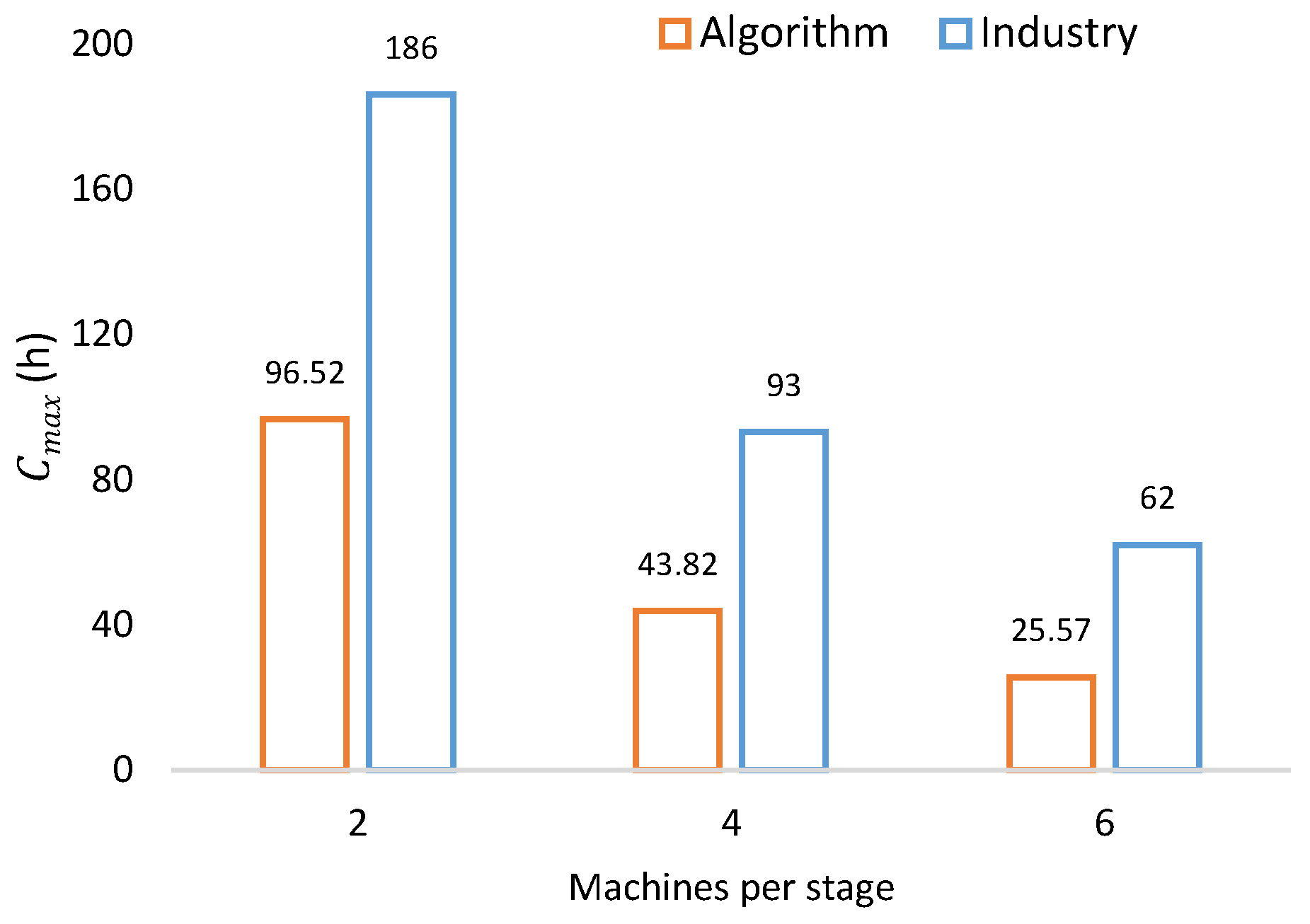
Table 19.
Results of the industry and B&B algorithm.
Table 19.
Results of the industry and B&B algorithm.
| Machines per Stage | Industry | B&B Algorithm |
|---|
| (kW) | (h) | (kW) | (h) |
|---|
| 2 | 13,050.90 | 186 | 6,831.40 | 96.52 |
| 4 | 26,101.80 | 93 | 12,206.42 | 43.82 |
| 6 | 39,152.70 | 62 | 16,828.72 | 25.57 |
Table 20.
The industry and bi-objective GA degradation over B&B algorithm (%).
Table 20.
The industry and bi-objective GA degradation over B&B algorithm (%).
| Machines per Stage | Industry | Bi-Objective GA |
|---|
| % | % | % | % |
|---|
| 2 | 47.65 | 48.11 | 1.53 | 0.17 |
| 4 | 53.24 | 52.88 | 0.87 | 0.54 |
| 6 | 57.02 | 58.75 | 0.62 | 0.47 |


 ,
, 


