Article

Learning Algorithm of Boltzmann Machine Based on Spatial Monte Carlo Integration Method

Graduate School of Science and Engineering, Yamagata University, Yamagata 992-8510, Japan
Algorithms 2018, 11(4), 42; https://doi.org/10.3390/a11040042
Submission received: 28 February 2018 / Revised: 2 April 2018 / Accepted: 3 April 2018 / Published: 4 April 2018
(This article belongs to the Special Issue Monte Carlo Methods and Algorithms)

Abstract

:
The machine learning techniques for Markov random fields are fundamental in various fields involving pattern recognition, image processing, sparse modeling, and earth science, and a Boltzmann machine is one of the most important models in Markov random fields. However, the inference and learning problems in the Boltzmann machine are NP-hard. The investigation of an effective learning algorithm for the Boltzmann machine is one of the most important challenges in the field of statistical machine learning. In this paper, we study Boltzmann machine learning based on the (first-order) spatial Monte Carlo integration method, referred to as the 1-SMCI learning method, which was proposed in the author’s previous paper. In the first part of this paper, we compare the method with the maximum pseudo-likelihood estimation (MPLE) method using a theoretical and a numerical approaches, and show the 1-SMCI learning method is more effective than the MPLE. In the latter part, we compare the 1-SMCI learning method with other effective methods, ratio matching and minimum probability flow, using a numerical experiment, and show the 1-SMCI learning method outperforms them.

1. Introduction

The machine learning techniques for Markov random fields (MRFs) are fundamental in various fields involving pattern recognition [1,2], image processing [3], sparse modeling [4], and Earth science [5,6], and a Boltzmann machine [7,8,9] is one of the most important models in MRFs. The inference and learning problems in the Boltzmann machine are NP-hard, because they include intractable multiple summations over all the possible configurations of variables. Thus, one of the major challenges of the Boltzmann machine is the design of the efficient inference and learning algorithms that it requires.
Various effective algorithms for Boltzmann machine learning were proposed by many researchers, a few of which are mean-field learning algorithms [10,11,12,13,14,15], maximum pseudo-likelihood estimation (MPLE) [16,17], contrastive divergence (CD) [18], ratio matching (RM) [19], and minimum probability flow (MPF) [20,21]. In particular, the CD and MPLE methods are widely used. More recently, the author proposed an effective learning algorithm based on the spatial Monte Carlo integration (SMCI) method [22]. The SMCI method is a Monte Carlo integration method that takes spatial information around the region of focus into account; it was proven that this method is more effective than the standard Monte Carlo integration method. The main target of this study is Boltzmann machine learning based on the first-order SMCI (1-SMCI) method, which is the simplest version of the SMCI method. We refer it to as the 1-SMCI learning method in this paper.
It was empirically shown through the numerical experiments that Boltzmann machine learning based on the 1-SMCI learning method is more effective than MPLE in the case where no model error exists, i.e., in the case where the learning model includes the generative model [22]. However, the theoretical reason for this was not revealed at all. In this paper, theoretical insights into the effectiveness of the 1-SMCI learning method as compared to that of MPLE are given from an asymptotic point of view. The theoretical results obtained in this paper state that the gradients of the log-likelihood function obtained by the 1-SMCI learning method constitute a quantitatively better approximation of the exact gradients than those obtained by the MPLE method in the case where the generative model and the learning model are the same Boltzmann machine (in Section 4.1). This is one of the contributions of this paper. In the previous paper [22], the 1-SMCI learning method was compared with only the MPLE. In this paper, we compare the 1-SMCI learning method with other effective learning algorithms, RM and MPF, through numerical experiments, and show that the 1-SMCI learning method is superior to them (in Section 5). This is the second contribution of this paper.
The remainder of this paper is organized as follows. The definition of Boltzmann machine learning and a briefly explanation of the MPLE method are given in Section 2. In Section 3, we explain Boltzmann machine learning based on the 1-SMCI method: reviews of the SMCI and 1-SMCI learning methods are presented in Section 3.1 and Section 3.2, respectively. In Section 4, the 1-SMCI learning method and MPLE are compared using two different approaches, the theoretical approach (in Section 4.1) and the numerical approach (in Section 4.2), and the effectiveness of the 1-SMCI learning method as compared to the MPLE is shown. In Section 5, we numerically compare the 1-SMCI method with other effective learning algorithms and observe that the 1-SMCI learning method yields the best approximation. Finally, the conclusion is given in Section 6.

2. Boltzmann Machine Learning

Consider an undirected and connected graph, G = ( V , E ) , with n nodes, where V : = { 1 , 2 , , n } is the set of labels of nodes and E is the set of labels of undirected links; an undirected link between nodes i and j is labeled ( i , j ) . Since an undirected graph is now considered, labels ( i , j ) and ( j , i ) indicate the same link. On undirected graph G, we define a Boltzmann machine with random variables x : = { x i X i V } , where X is the sample space of the variable. It is expressed as [7,9]
P BM ( x w ) : = 1 Z ( w ) exp ( i , j ) E w i j x i x j ,
where Z ( w ) is the partition function defined by
Z ( w ) : = x exp ( i , j ) E w i j x i x j ,
where x is the multiple summation over all the possible realizations of x ; i.e., x = i V x i X . Here and in the following, if x i is continuous, x i X is replaced by integration. w : = { w i j ( , ) ( i , j ) E } represents the symmetric coupling parameters ( w i j = w j i ). Although a Boltzmann machine can include a bias term, e.g., i V b i x i , in its exponent, it is ignored in this paper for the sake of the simplicity of arguments.
Suppose that a set of N data points corresponding to x , D : = { x ( μ ) μ = 1 , 2 , , N } where x ( μ ) : = { x i ( μ ) X i V } , is obtained. The goal of Boltzmann machine learning is to maximize the log-likelihood
l ( w ; D ) : = 1 N μ = 1 N ln P BM ( x ( μ ) w )
with respect to w , that is, the maximum likelihood estimation (MLE). The Boltzmann machine, with w that maximizes Equation (2), yields the distribution most similar to the data distribution (also referred to as the empirical distribution) in the perspective of the measure based on Kullback–Leibler divergence (KLD). This fact can be easily seen in the following. The empirical distribution of D is expressed as
Q D ( x ) : = 1 N μ = 1 N i V δ ( x i , x i ( μ ) ) ,
where δ ( a , b ) is the Kronecker delta function: δ ( a , b ) = 1 when a = b , and δ ( a , b ) = 0 when a b . The KLD between the empirical distribution and the Boltzmann machine in Equation (1),
D KL [ Q D P BM ] : = x Q D ( x ) ln Q D ( x ) P BM ( x w ) ,
can be rewritten as D KL [ Q D P BM ] = l ( w ; D ) + C , where C is the constant unrelated to w . From this equation, we determine that w that maximizes the log-likelihood in Equation (2) minimizes the KLD.
Since the log-likelihood in Equation (2) is the concave function with respect to w [8], in principle, we can optimize the log-likelihood using a gradient ascent method. The gradient of the log-likelihood with respect to w i j is
Δ i j M L E ( w ; D ) : = l ( w ; D ) w i j = 1 N μ = 1 N x i ( μ ) x j ( μ ) E BM [ x i x j w ] ,
where E BM [ w ] : = x ( ) P BM ( x w ) is the expectation of the assigned quantity over the Boltzmann machine in Equation (1). In the optimal point of the MLE, all the gradients are zero, and therefore, from Equation (5), the optimal w is the solution to the simultaneous equations
1 N μ = 1 N x i ( μ ) x j ( μ ) = E BM [ x i x j w ] .
When the data points are generated independently from a Boltzmann machine, P BM ( x w g e n ) , defined on the same graph as the Boltzmann machine we use in the learning, i.e., the case without the model error, the solution to the MLE, w MLE , converges to w gen as N [23]. In other words, the MLE is asymptotically consistent.
However, it is difficult to compute the second term in Equation (5), because the computations of these expectations need the summation over O ( 2 n ) terms. Thus, the exact Boltzmann machine learning, i.e., the MLE, cannot be performed. As mentioned in Section 1, various approximations for Boltzmann machine learning were proposed by many authors, such as the mean-field learning methods [10,11,12,13,14,15] and the MPLE [16,17], CD [18], RM [19], MPF [20,21] and SMCI [22] methods. In the following, we briefly review the MPLE method.
In MPLE, we maximize the following pseudo-likelihood [16,17,24] instead of the true log-likelihood in Equation (2).
l MPLE ( w ; D ) : = 1 N μ = 1 N i V ln P BM ( x i ( μ ) x { i } ( μ ) , w ) ,
where x A : = { x i i A V } is the variables in A and A : = V A ; i.e., x { i } = x { x i } 
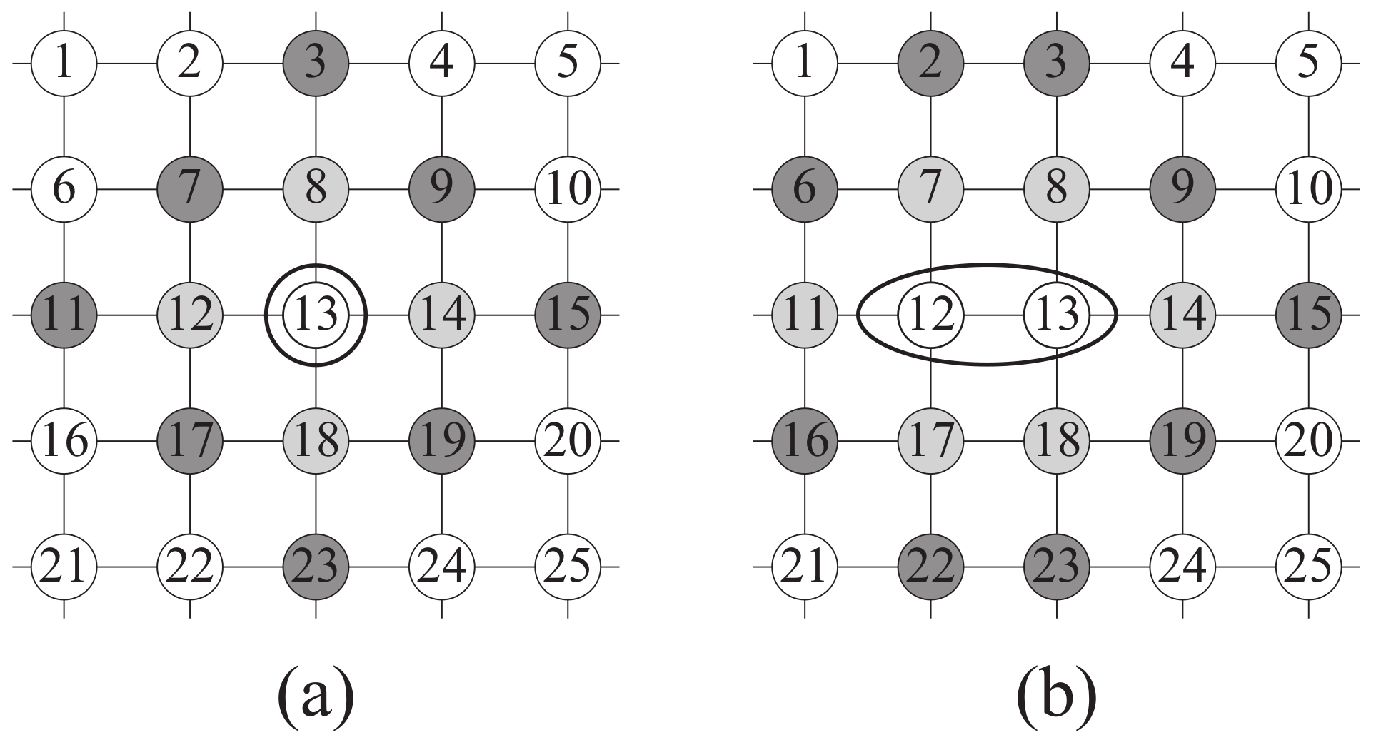
. The conditional distribution in the above equation is the conditional distribution in the Boltzmann machine expressed by
P BM ( x i x { i } , w ) = P BM ( x w ) x i X P BM ( x w ) = exp U i ( x ( i ) , w ) x i x i X exp U i ( x ( i ) , w ) x i ,
where
U i ( x ( i ) , w ) : = j ( i ) w i j x j ,
where ( i ) V is the set of labels of nodes directly connected to node i; i.e., ( i ) : = { j ( i , j ) E } . The derivative of the pseudo-likelihood with respect to w i j is
l MPLE ( w ; D ) w i j = 2 1 N μ = 1 N x i ( μ ) x j ( μ ) m i j MPLE ( w ; D ) .
m i j MPLE ( w ; D ) is defined by
m i j MPLE ( w ; D ) : = 1 2 N μ = 1 N x j ( μ ) M i ( x ( i ) ( μ ) , w ) + x i ( μ ) M j ( x ( j ) ( μ ) , w ) ,
where
M i ( x ( i ) , w ) : = x i X x i exp U i ( x ( i ) , w ) x i x i X exp U i ( x ( i ) , w ) x i
and where, for a set A V , x A ( μ ) is the μ -th data point corresponding to x A ; i.e., x A ( μ ) = { x i ( μ ) i A V } . When X = { 1 , + 1 } , M i ( x ( i ) , w ) = tanh U i ( x ( i ) , w ) . In order to fit the magnitude of the gradient to that of the MLE, we use half of Equation (10) as the gradient of the MPLE
Δ i j MPLE ( w ; D ) : = 1 N μ = 1 N x i ( μ ) x j ( μ ) m i j MPLE ( w ; D ) .
The order of the total computational complexity of the gradients in Equation (11) is O ( N | E | ) , where | E | is the number of links in G ( V , E ) . The pseudo-likelihood is also the concave function with respect to w , and therefore, one can optimize it using a gradient ascent method. The typical performance of the MPLE method is almost the same as or slightly better than that of the CD method in Boltzmann machine learning [24].
From Equation (13), the optimal w in the MPLE is the solution to the simultaneous equations
1 N μ = 1 N x i ( μ ) x j ( μ ) = m i j MPLE ( w ; D ) .
By comparing Equation (6) with Equation (14), it can be seen that the MPLE is the approximation of the MLE such that E BM [ x i x j w ] m i j MPLE ( w ; D ) . Many authors proved that the MPLE is also asymptotically consistent (for example, [24,25,26]), that is, in the case without model error, the solution to the MPLE, w MPLE , converges to w gen as N . However, the asymptotic variance of the MPLE is larger than that of the MLE [25].

3. Boltzmann Machine Learning Based on Spatial Monte Carlo Integration Method

In this section, we present the reviews of both the SMCI method and the application of the first-order of the SMCI method to Boltzmann machine learning, i.e., the 1-SMCI learning method.

3.1. Spatial Monte Carlo Integration Method

Assume that we have a set of i.i.d. sample points, S : = { s ( μ ) μ = 1 , 2 , , N } , where s ( μ ) : = { s i ( μ ) X i V } , drawn from a Boltzmann machine, P BM ( x w ) , by using a Markov chain Monte Carlo (MCMC) method. Suppose that we want to know the expectation of a function f ( x C ) , C V , for the Boltzmann machine E BM [ f ( x C ) w ] . In the standard Monte Carlo integration (MCI) method, we approximate the desired expectation by the simple average of the given sample points S :
E BM [ f ( x C ) w ] x f ( x C ) Q S ( x ) = 1 N μ = 1 N f ( s C ( μ ) ) ,
where Q S ( x ) is the distribution of the sample points, which is defined in the same manner as Equation (3), and where, for a set A V , s A ( μ ) is the μ -th sample point corresponding to x A ; i.e., s A ( μ ) = { s i ( μ ) i A V } .
The SMCI method considers spatial information around x C , in contrast to the standard MCI method. For the SMCI method, we define the neighboring regions of the target region, C V , as follows. The first-nearest-neighbor region, N 1 ( C ) , is defined by
N 1 ( C ) : = { i ( i , j ) E , j C , i C } .
Therefore, when C = { i } , N 1 ( C ) = ( i ) . Similarly, the second-nearest-neighbor region, N 2 ( C ) , is defined by
N 2 ( C ) : = { i ( i , j ) E , j N 1 ( C ) , i C , i N 1 ( C ) } .
In a similar manner, for k 1 , we define the k-th-nearest-neighbor region, N k ( C ) , by
N k ( C ) : = { i ( i , j ) E , j N k 1 ( C ) , i R k 1 ( C ) } ,
where R k ( C ) : = m = 0 k N m ( C ) and N 0 ( C ) : = C . An example of the neighboring regions in a square-grid graph is shown in Figure 1.
By using the conditional distribution,
P BM ( x R k 1 ( C ) x N k ( C ) , w ) = P BM ( x w ) x R k 1 ( C ) P BM ( x w ) ,
and the marginal distribution,
P BM ( x N k ( C ) w ) = x V N k ( C ) P BM ( x w ) ,
the desired expectation can be expressed as
E BM [ f ( x C ) w ] = x R k 1 ( C ) x N k ( C ) f ( x C ) P BM ( x R k 1 ( C ) x N k ( C ) , w ) P BM ( x N k ( C ) w ) ,
where, for a set A V , x A = i A x i X . In Equation (19), we used the Markov property of the Boltzmann machine:
P BM ( x R k 1 ( C ) x V R k 1 ( C ) , w ) = P BM ( x R k 1 ( C ) x N k ( C ) , w ) .
In the k-th-order SMCI (k-SMCI) method, E BM [ f ( x C ) w ] in Equation (21) is approximated by
E k [ f ( x C ) w , S ] : = x R k 1 ( C ) x N k ( C ) f ( x C ) P BM ( x R k 1 ( C ) x N k ( C ) , w ) Q S ( x ) = 1 N μ = 1 N x R k 1 ( C ) f ( x C ) P BM ( x R k 1 ( C ) s N k ( C ) ( μ ) , w ) .
The k-SMCI method takes the spatial information up to the ( k 1 ) -th-nearest-neighbor region into account, and it approximates the outside of it (namely, the k-th-nearest-neighbor region) by the sample distribution. For the SMCI method, two important facts were theoretically proven [22]: (i) the SMCI method is asymptotically better than the standard MCI method and (ii) a higher-order SMCI method is better asymptotically than a lower-order one.

3.2. Boltzmann Machine Learning Based on First-Order SMCI Method

Applying the 1-SMCI method to Boltzmann machine learning is achieved by approximating the intractable expectations, E BM [ x i x j w ] , by the 1-SMCI method in Equation (22) with k = 1 . Although Equation (22) requires sample points S drawn from P BM ( x w ) , as discussed in the previous section, we can avoid the sampling by using dataset D instead of S [22]. We approximate E BM [ x i x j w ] by
m i j 1 SMCI ( w ; D ) : = E 1 [ x { i , j } w , D ] = 1 N μ = 1 N x i , x j X x i x j P BM ( x i , x j x N 1 ( { i , j } ) ( μ ) , w ) .
Since
P BM ( x i , x j x N 1 ( { i , j } ) ( μ ) , w ) exp U i ( x ( i ) ( μ ) , w ) w i j x j ( μ ) x i + U j ( x ( j ) ( μ ) , w ) w j i x i ( μ ) x j + w i j x i x j ,
the order of the computational complexity of e i j 1 SMCI ( w ; D ) is the same as that of m i j MPLE ( w ; D ) with respect to n. For example, when X = { 1 , + 1 } , Equation (23) becomes
m i j 1 SMCI ( w ; D ) = 1 N μ = 1 N tanh tanh 1 tanh U i ( x ( i ) ( μ ) , w ) w i j x j ( μ ) tanh U j ( x ( j ) ( μ ) , w ) w j i x i ( μ ) + w i j ,
where tanh 1 ( x ) is the inverse function of tanh ( x ) .
By using the 1-SMCI learning method, the true gradient, Δ i j MLE ( w ; D ) , is thus approximated as
Δ i j 1 SMCI ( w ; D ) : = 1 N μ = 1 N x i ( μ ) x j ( μ ) m i j 1 SMCI ( w ; D ) ,
and therefore, the optimal w in this approximation is the solution to the simultaneous equations:
1 N μ = 1 N x i ( μ ) x j ( μ ) = m i j 1 SMCI ( w ; D ) .
The order of the total computational complexity of the gradients in Equation (23) is O ( N | E | ) , which is the same as that of the MPLE. The solution to Equation (27) is obtained by a gradient ascent method with the gradients in Equation (26).

4. Comparison of 1-SMCI Learning Method and MPLE

It was empirically observed in some numerical experiments that the 1-SMCI learning method discussed in the previous section is better than MPLE in the case without model error [22]. In this section, first we provide some theoretical insights into this observation, and then some numerical comparisons of the two methods in the cases with and without model error.

4.1. Comparison from Asymptotic Point of View

Suppose that we want to approximate the expectation E BM [ x i x j w ] in a Boltzmann machine, and assume that the data points are generated independently from the same Boltzmann machine. Here, we re-express m i j MPLE ( w ; D ) in Equation (11) and m i j 1 SMCI ( w ; D ) in Equation (23) as
m i j MPLE ( w ; D ) = 1 N μ = 1 N ρ i j MPLE ( x ( μ ) , w ) ,
m i j 1 SMCI ( w ; D ) = 1 N μ = 1 N ρ i j 1 SMCI ( x ( μ ) , w ) ,
respectively, where
ρ i j MPLE ( x , w ) : = 1 2 x j M i ( x ( i ) , w ) + x i M j ( x ( j ) , w ) , ρ i j 1 SMCI ( x , w ) : = x i X x j X x i x j P BM ( x i , x j x N 1 ( { i , j } ) , w ) .
Since x ( μ ) s are the i.i.d. points sampled from P BM ( x w ) , ρ i j MPLE ( x ( μ ) , w ) and ρ i j 1 SMCI ( x ( μ ) , w ) can also be regarded as i.i.d. sample points. Thus, m i j MPLE ( w ; D ) and m i j 1 SMCI ( w ; D ) are the sample averages over the i.i.d. points. One can easily verify that the two equations x P BM ( x w ) ρ i j MPLE ( x , w ) = E BM [ x i x j w ] and x P BM ( x w ) ρ i j 1 SMCI ( x , w ) = E BM [ x i x j w ] are justified (the former equation can also be justified by using the correlation equality [27]). Therefore, from the law of large numbers, m i j MPLE ( w ; D ) = m i j 1 SMCI ( w ; D ) = E BM [ x i x j w ] in the limit of N . This implies that, in the case without model error, the 1-SMCI learning method has the same solution to the MLE in the limit of N .
From the central limit theorem, the distributions of m i j MPLE ( w ; D ) and m i j 1 SMCI ( w ; D ) asymptotically converge to Gaussians with mean E BM [ x i x j w ] and variances
v i j MPLE ( w ) : = 1 N x ρ i j MPLE ( x , w ) 2 P BM ( x w ) E BM [ x i x j w ] 2 ,
v i j 1 SMCI ( w ) : = 1 N x ρ i j SMCI ( x , w ) 2 P BM ( x w ) E BM [ x i x j w ] 2 ,
respectively, for N 1 . For the two variances, we obtain the following theorem.
Theorem 1.
For a Boltzmann machine, P BM ( x w ) , defined in Equation (1), the inequality v i j MPLE ( w ) v i j 1 SMCI ( w ) is satisfied for all ( i , j ) E and for any N.
The proof of this theorem is given in Appendix A. Theorem 1 states that the variance in the distribution of m i j MPLE ( w ; D ) is always larger than (or equal to) that of m i j 1 SMCI ( w ; D ) . This means that, when N 1 , the distribution of m i j 1 SMCI ( w ; D ) converges to a Gaussian around the mean value (i.e., the exact expectation) that is sharper than a Gaussian to which the distribution of m i j MPLE ( w ; D ) converges, and therefore, it is likely that m i j 1 SMCI ( w ; D ) is closer to the exact expectation than m i j MPLE ( w ; D ) when N 1 ; that is, m i j 1 SMCI ( w ; D ) is a better approximation of E BM [ x i x j w ] than m i j MPLE ( w ; D ) .
Next, we consider the differences between the true gradient in Equation (5) and the approximate gradients in Equations (13) and (26) for w i j :
e i j MPLE ( w ; D ) : = Δ i j MPLE ( w ; D ) Δ i j MLE ( w ; D ) = m i j MPLE ( w ; D ) E BM [ x i x j w ] ,
e i j 1 SMCI ( w ; D ) : = Δ i j 1 SMCI ( w ; D ) Δ i j MLE ( w ; D ) = m i j 1 SMCI ( w ; D ) E BM [ x i x j w ] .
For the gradient differences in Equations (32) and (33), we obtain the following theorem.
Theorem 2.
For a Boltzmann machine, P BM ( x w ) , defined in Equation (1), the inequality
P | e i j MPLE ( w ; D ) | ε P | e i j 1 SMCI ( w ; D ) | ε , ε > 0 ,
is satisfied for all ( i , j ) E when N , where D is the set of N data points generated independently from P BM ( x w ) .
The proof of this theorem is given in Appendix B. Theorem 2 states that it is likely that the magnitude of e i j 1 SMCI ( w ; D ) is smaller than (or equivalent to) that of e i j MPLE ( w ; D ) when the data points are generated independently from the same Boltzmann machine and when N 1 .
Suppose that N data points are generated independently from a generative Boltzmann machine, P BM ( x w gen ) , defined on G gen , and that a learning Boltzmann machine, defined on the same graph as the generative Boltzmann machine, is trained using the generative data points. In this case, since there is no model error, the solutions of the MLE, the MPLE and the 1-SMCI learning methods are expected to approach w gen as N , that is Δ i j MLE ( w gen ; D ) , Δ i j MPLE ( w gen ; D ) , and Δ i j 1 SMCI ( w gen ; D ) are expected to approach zero as N . Consider the case in which N is very large and Δ i j MLE ( w gen ; D ) = 0 . From the statement in Theorem 2, Δ i j 1 SMCI ( w gen ; D ) is statistically closer to zero than Δ i j MPLE ( w gen ; D ) . This implies that the solution of the 1-SMCI learning method converges to that of the MLE faster than the MPLE.
The theoretical results presented in this section have not reached a rigid justification of the effectiveness of the 1-SMCI learning method, because some issues still remain, for instance: (i) since we do not specify whether the problem of solving Equation (27), i.e., a gradient ascent method with the gradients in Equation (26), is a convex problem or not, we cannot remove the possibility of existence local optimal solutions which degrade the performance of the 1-SMCI learning method, (ii) although we discussed the asymptotic property of Δ i j 1 SMCI ( w ; D ) for each link separately, a joint analysis of them is necessary for a more rigid discussion, and (iii) a perturbative analysis around the optimal point is completely lacking. However, we can expect that they constitute evidence that is important for gaining insight into the effectiveness.

4.2. Numerical Comparison

We generated N data points from a generative Boltzmann machine, P BM ( x w gen ) and then trained a learning Boltzmann machine of the same size as the generative Boltzmann machine using the generated data points. The coupling parameters in the generative Boltzmann machine, w gen , were generated from a unique distribution, U [ λ , λ ] .
First, we consider the case where the graph structures of the generative Boltzmann machine and the learning Boltzmann machine are the same: a 4 × 4 square grid, that is the case “without” model error. 
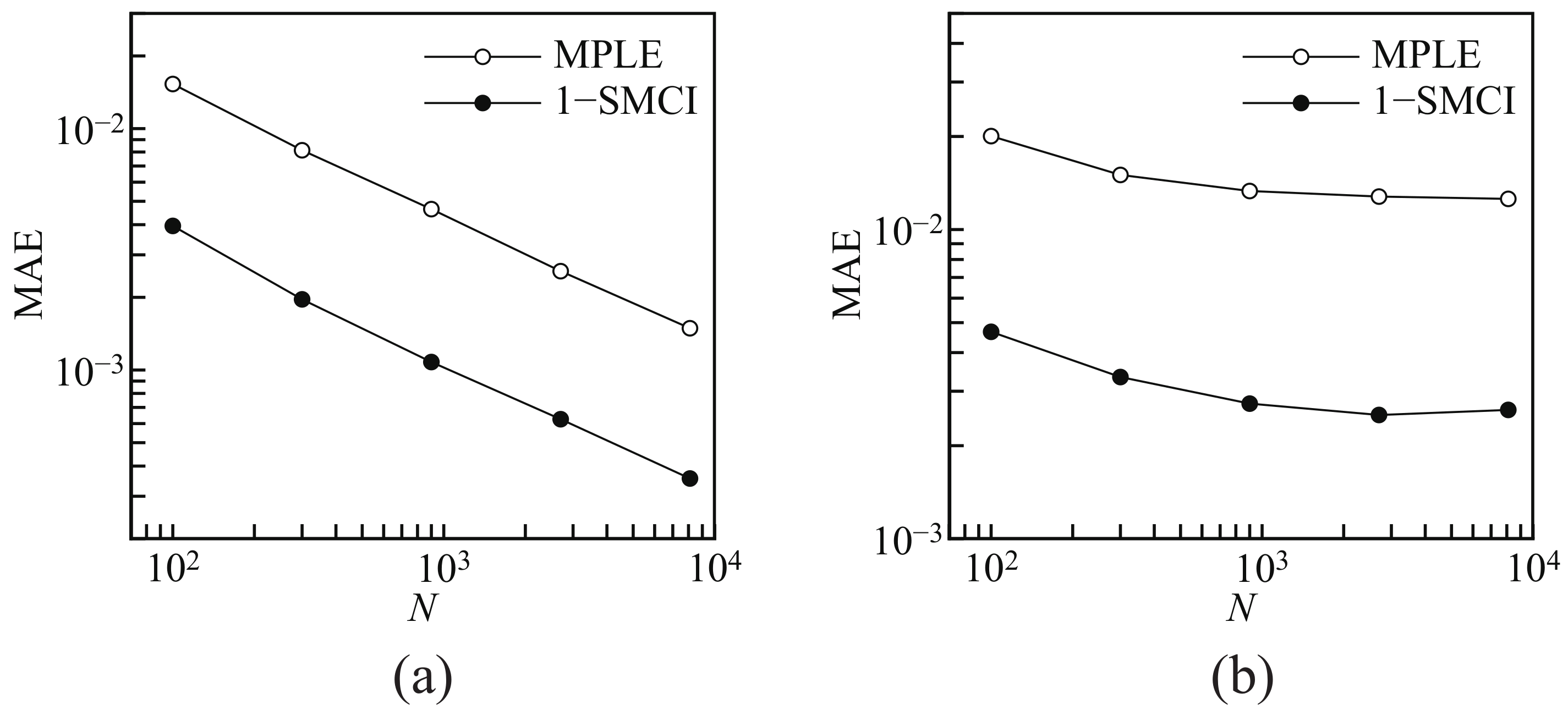
Figure 2a shows the mean absolute errors between the solutions to the MLE and the approximate methods (the MLPE and the 1-SMCI learning method), ( i , j ) E | w i j MLE w i j approx | / | E | , against N. Here, we set λ = 0.3 . Since the size of the Boltzmann machine used here is not large, we can obtain the solution to the MLE. We observe that the solutions to the two approximate methods converge to the solution to the MLE as N increases, and the 1-SMCI learning method is better than the MPLE as the approximation of the MLE. These results are consistent with the results obtained in [22] and the theoretical arguments in the previous section.
Next, we consider the case in which the graph structure of the generative Boltzmann machine is fully connected with n = 16 and that in which the learning Boltzmann machine is again a 4 × 4 square grid, namely the case “with” model error. Thus, this case is completely outside the theoretical arguments in the previous section. Figure 2b shows the mean absolute errors between the solution to the MLE and that to the approximate methods against N. Here, we set λ = 0.2 . Unlike the above case, the solutions to the two approximate methods do not converge to the solution to the MLE because of the model error. The 1-SMCI learning method is again better than the MPLE as the approximation of the MLE in this case.
By comparing Figure 2a,b, we observed that the 1-SMCI learning method in (b) is worse than in (a). The following reason can be considered. In Section 3.2, we replaced S , which is the sample points drawn from the Boltzmann machine, by D in order to avoid the sampling cost. However, this replacement implies the assumption of the case “without” model error, and therefore, it is not justified in the case “with” model error.

5. Numerical Comparison with Other Methods

In this section, we demonstrate a numerical comparison of the 1-SMCI learning method with other approximation methods, RM [19] and MPF [20,21]. The orders of the computational complexity of these two methods are the same as that of the MPLE and 1-SMCI learning methods. The four methods were implemented by a simple gradient ascent method, w i j ( t + 1 ) w i j ( t ) + η Δ i j , where η > 0 is the learning rate.
As described in Section 4.2, we generated N data points from a generative Boltzmann machine, P BM ( x w gen ) and then trained a learning Boltzmann machine of the same size as the generative Boltzmann machine using the generated data points. The coupling parameters in the generative Boltzmann machine, w gen , were generated from U [ 0.3 , 0.3 ] . The graph structures of the generative Boltzmann machine and of the learning Boltzmann machine are the same: a 4 × 4 square grid. 
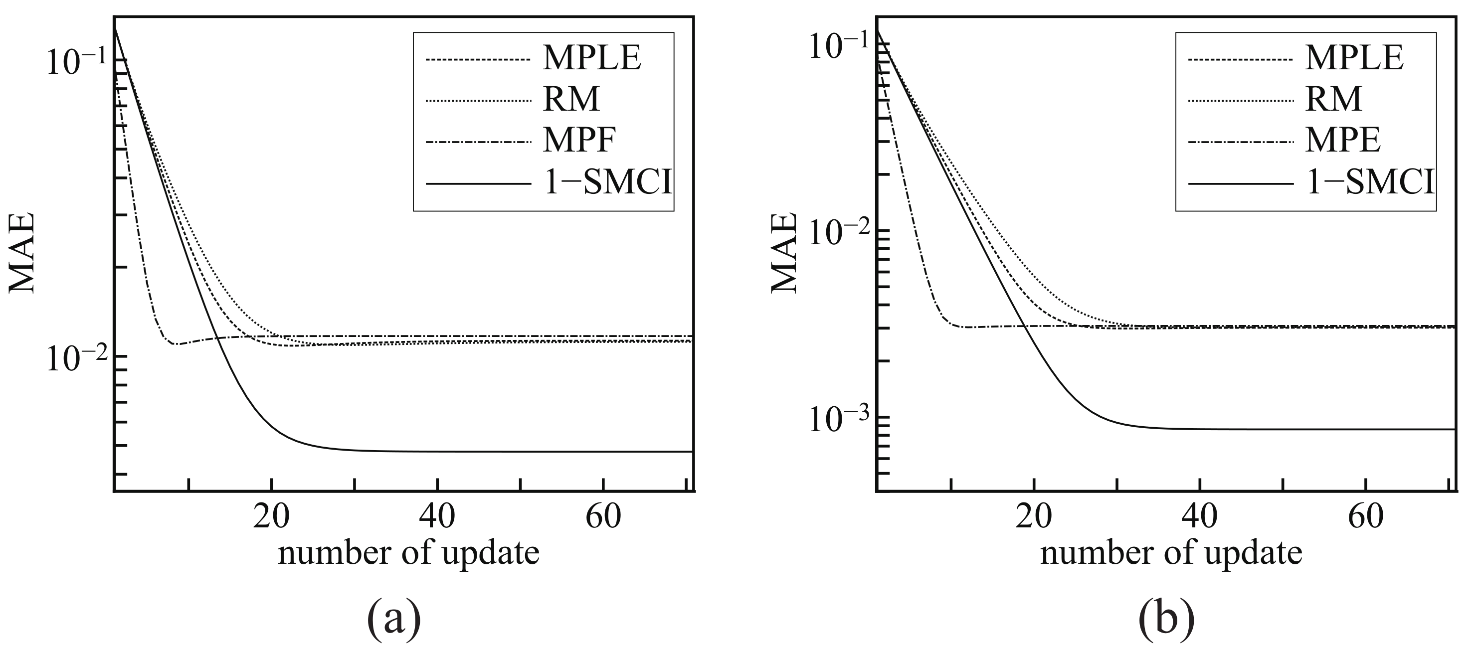
Figure 3 shows the learning curves of the four methods. The horizontal axis represents the number of the step, t, of the gradient ascent method, and the vertical axis represents the mean absolute errors between the solution to the MLE, w MLE , and the values of the coupling parameters at the step, w ( t ) . In this experiment, we set η = 0.2 , and the values of w were initialized as zero.
Since the vertical axises in Figure 3 represents the the mean absolute error from the solution to the MLE, the lower one is the better approximation of the MLE. We can observe that the MPF shows the fastest convergence and the MPLE, RM, and MPF converge to almost the same values, while the 1-SMCI learning method converges to the lowest values. This concludes that, among the four methods, the 1-SMCI learning method is the best as the approximation of the MLE. However, the 1-SMCI learning method has a drawback. The MPLE, RM, and MPF are convex optimization problems and they have unique solutions, whereas, we do not specify whether the 1-SMCI learning method is a convex problem or not in the present stage. We cannot eliminate the possibility of the existence of local optimal solutions that degrade the accuracy of approximation.
As mentioned above, the orders of the computational complexity of these four methods, the MPLE, RM, MPF, and 1-SMCI learning methods, are the same, O ( N | E | ) . However, it is important to check the real computational times of these methods. Table 1 shows the total computational times needed for the one-time learning (until convergence), where the setting of the experiment is the same as that of Figure 3b.
The MPF method is the fastest, and the 1-SMCI learning method is the slowest which is about 6–7 times slower than the MPF method.

6. Conclusions

In this paper, we examined the effectiveness of Boltzmann machine learning based on the 1-SMCI method proposed in [22] where, by numerical experiments, it was shown that the 1-SMCI learning method is more effective than the MPLE in the case where no model error exists. In Section 4.1, we gave the theoretical results for the empirical observation from the asymptotic point of view. The theoretical results improved our understanding of the advantage of the 1-SMCI learning method as compared to the MPLE. The numerical experiments in Section 4.2 showed that the 1-SMCI learning method is a better approximation of the MPLE in the case with and without model error. Furthermore, we compared the 1-SMCI learning method with the other effective methods, RM and MPF, using the numerical experiments in Section 5. The numerical results showed that the 1-SMCI learning method is the best method.
However, issues related to the 1-SMCI learning method still remain. Since the objective function of the 1-SMCI learning method, e.g., Equation (7) for the MPLE, is not revealed, it is not straightforward to specify whether the problem of solving Equation (27), i.e., a gradient ascent method with the gradients in Equation (26), is a convex problem or not. This is one of the most challenging issues of the method. As shown in Section 4.2, the performance of the 1-SMCI learning method decreases when model error exists, i.e., when the learning Boltzmann machine does not include the generative model. The decrease may be caused by the replacement of the sample points, S , by the data points, D , as discussed in the same section. It is expected that combining the 1-SMCI learning method with an effective sampling method, e.g., the persistent contrastive divergence [28], relaxes the problem of the performance degradation.
The presented the 1-SMCI learning method can be applied to other types of Boltzmann machines, e.g., restricted Boltzmann machine [1], deep Boltzmann machine [2,29]. Although we focused on the Boltzmann machine learning in this paper, the SMCI method can be applied to various MRFs [22]. Hence, there are many future directions of application of the SMCI: for example, graphical LASSO problem [4], Bayesian image processing [3], Earth science [5,6] and brain-computer interface [30,31,32,33].

Acknowledgments

This work was partially supported by JST CREST, Grant Number JPMJCR1402, JSPS KAKENHI, Grant Numbers, 15K00330 and 15H03699, and MIC SCOPE (Strategic Information and Communications R&D Promotion Programme), Grant Number 172302009.

Conflicts of Interest

The author declares no conflict of interest.

Appendix A. Proof of Theorem 1

The first term in Equation (30) can be rewritten as:
x ρ i j MPLE ( x , w ) 2 P BM ( x w ) = x x i X x j X ρ i j MPLE ( x , w ) 2 P BM ( x i , x j x N 1 ( { i , j } ) , w ) P BM ( x w ) .
Since, for ( i , j ) E , x N 1 ( { i , j } ) = x N 1 ( { i } ) x N 1 ( { j } ) { x i , x j } , we obtain the two expressions:
P BM ( x i , x j x N 1 ( { i , j } ) , w ) = P BM ( x i x j , x N 1 ( { i , j } ) , w ) P BM ( x j x N 1 ( { i , j } ) , w ) = P BM ( x i x N 1 ( { i } ) , w ) P BM ( x j x N 1 ( { i , j } ) , w )
and the expression, obtained by alternating i and j,
P BM ( x i , x j x N 1 ( { i , j } ) , w ) = P BM ( x j x N 1 ( { j } ) , w ) P BM ( x i x N 1 ( { i , j } ) , w ) .
From Equations (A2) and (A3), we obtain:
ρ i j SMCI ( x , w ) = 1 2 x i X x i M j ( x ( j ) , w ) P BM ( x i x N 1 ( { i , j } ) , w ) + x j X x j M i ( x ( i ) , w ) P BM ( x j x N 1 ( { i , j } ) , w ) = x i X x j X ρ i j MPLE ( x , w ) P BM ( x i , x j x N 1 ( { i , j } ) , w ) ,
where we use the relation M i ( x ( i ) , w ) = x i X x i P BM ( x i x N 1 ( { i } ) , w ) . From this equation, we obtain
x ρ i j 1 SMCI ( x , w ) 2 P BM ( x w ) = x x i X x j X ρ i j MPLE ( x , w ) P BM ( x i , x j x N 1 ( { i , j } ) , w ) 2 P BM ( x w ) .
Finally, from Equations (A1) and (A5), the inequality:
v i j MPLE ( w ) v i j 1 SMCI ( w ) = 1 N x { x i X x j X ρ i j MPLE ( x , w ) 2 P BM ( x i , x j x N 1 ( { i , j } ) , w ) x i X x j X ρ i j MPLE ( x , w ) P BM ( x i , x j x N 1 ( { i , j } ) , w ) 2 } P BM ( x w ) 0
is obtained.

Appendix B. Proof of Theorem 2

As mentioned in Section 4.1, from the central limit theorem, the distribution of m i j MPLE ( w ; D ) converges to the Gaussian with mean E BM [ x i x j w ] and variance v i j MPLE ( w ) for N . Therefore, the distribution of e i j MPLE ( w ; D ) converges to the Gaussian with mean zero and variance v i j MPLE ( w ) . This leads to
P | e i j MPLE ( w ; D ) | ε = P ε e i j MPLE ( w ; D ) ε ε ε N ( t v i j MPLE ( w ) ) d t ( N ) ,
where N ( t σ 2 ) : = exp { t 2 / ( 2 σ 2 ) } / 2 σ 2 . Equation (A7) is expressed as:
ε ε N ( t v i j MPLE ( w ) ) d t = erf ε 2 v i j MPLE ( w )
by using the error function
erf ( x ) : = 1 π x x e t 2 d t .
We obtain
P | e i j 1 SMCI ( w ; D ) | ε erf ε 2 v i j 1 SMCI ( w ) ( N )
by using the same derivation as Equation (A8). Because the error function in Equation (A9) is the monotonically increasing function, from the statement in Theorem 1, i.e., v i j MPLE ( w ) v i j 1 SMCI ( w ) , we obtain
erf ε 2 v i j MPLE ( w ) erf ε 2 v i j 1 SMCL ( w ) .
This inequality leads to the statement of Theorem 2.

References

  1. Hinton, G.E.; Osindero, S.; Teh, Y.W. A fast learning algorithm for deep belief net. Neural Comput. 2006, 18, 1527–1554. [Google Scholar] [CrossRef] [PubMed]
  2. Salakhutdinov, R.; Hinton, G.E. An Efficient Learning Procedure for Deep Boltzmann Machines. Neural Comput. 2012, 24, 1967–2006. [Google Scholar] [CrossRef] [PubMed]
  3. Blake, A.; Kohli, P.; Rother, C. Markov Random Fields for Vision and Image Processing; The MIT Press: Cambridge, MA, USA, 2011. [Google Scholar]
  4. Rish, I.; Grabarnik, G. Sparse Modeling: Theory, Algorithms, and Applications; CRC Press: Boca Raton, FL, USA, 2014. [Google Scholar]
  5. Kuwatani, T.; Nagata, K.; Okada, M.; Toriumi, M. Markov random field modeling for mapping geofluid distributions from seismic velocity structures. Earth Planets Space 2014, 66, 5. [Google Scholar] [CrossRef]
  6. Kuwatani, T.; Nagata, K.; Okada, M.; Toriumi, M. Markov-random-field modeling for linear seismic tomography. Phys. Rev. E 2014, 90, 042137. [Google Scholar] [CrossRef] [PubMed]
  7. Ackley, D.H.; Hinton, G.E.; Sejnowski, T.J. A learning algorithm for Boltzmann machines. Cogn. Sci. 1985, 9, 147–169. [Google Scholar] [CrossRef]
  8. Wainwright, M.J.; Jordan, M.I. Graphical Models, Exponential Families, and Variational Inference. Found. Trends Mach. Learn. 2008, 1, 1–305. [Google Scholar] [CrossRef]
  9. Murphy, K.P. Machine Learning: A Probabilistic Perspective; MIT Press: Cambridge, MA, USA, 2013. [Google Scholar]
  10. Kappen, H.J.; Rodríguez, F.B. Efficient Learning in Boltzmann Machines Using Linear Response Theory. Neural Comput. 1998, 10, 1137–1156. [Google Scholar] [CrossRef] [Green Version]
  11. Tanaka, T. Mean-field theory of Boltzmann machine learning. Phys. Rev. E 1998, 58, 2302–2310. [Google Scholar] [CrossRef]
  12. Yasuda, M.; Tanaka, K. Approximate Learning Algorithm in Boltzmann Machines. Neural Comput. 2009, 21, 3130–3178. [Google Scholar] [CrossRef] [PubMed]
  13. Sessak, V.; Monasson, R. Small-correlation expansions for the inverse Ising problem. J. Phys. A Math. Theor. 2009, 42, 055001. [Google Scholar] [CrossRef]
  14. Furtlehner, C. Approximate inverse Ising models close to a Bethe reference point. J. Stat. Mech. Theor. Exp. 2013, 2013, P09020. [Google Scholar] [CrossRef]
  15. Roudi, Y.; Aurell, E.; Hertz, J. Statistical physics of pairwise probability models. Front. Comput. Neurosci. 2009, 3, 22. [Google Scholar] [CrossRef] [PubMed]
  16. Besag, J. Statistical Analysis of Non-Lattice Data. J. R. Stat. Soc. D 1975, 24, 179–195. [Google Scholar] [CrossRef]
  17. Aurell, E.; Ekeberg, M. Inverse Ising Inference Using All the Data. Phys. Rev. Lett. 2012, 108, 090201. [Google Scholar] [CrossRef] [PubMed]
  18. Hinton, G.E. Training products of experts by minimizing contrastive divergence. Neural Comput. 2002, 8, 1771–1800. [Google Scholar] [CrossRef] [PubMed]
  19. Hyvärinen, A. Estimation of non-normalized statistical models using score matching. J. Mach. Learn. Res. 2005, 6, 695–709. [Google Scholar]
  20. Sohl-Dickstein, J.; Battaglino, P.B.; DeWeese, M.R. Minimum Probability Flow Learning. In Proceedings of the 28th International Conference on International Conference on Machine Learning (ICML’11), Bellevue, WA, USA, 28 June – 2 July 2011; pp. 905–912. [Google Scholar]
  21. Sohl-Dickstein, J.; Battaglino, P.B.; DeWeese, M.R. New Method for Parameter Estimation in Probabilistic Models: Minimum Probability Flow. Phys. Rev. Lett. 2011, 107, 220601. [Google Scholar] [CrossRef] [PubMed]
  22. Yasuda, M. Monte Carlo Integration Using Spatial Structure of Markov Random Field. J. Phys. Soc. Japan 2015, 84, 034001. [Google Scholar] [CrossRef]
  23. Lehmann, E.L.; Casella, G. Theory of Point Estimation; Springer: Berlin, Germany, 1998. [Google Scholar]
  24. Hyvärinen, A. Consistency of Pseudo likelihood Estimation of Fully Visible Boltzmann Machines. Neural Comput. 2006, 18, 2283–2292. [Google Scholar] [CrossRef] [PubMed]
  25. Lindsay, B.G. Composite Likelihood Methods. Contemporary Math. 1988, 80, 221–239. [Google Scholar]
  26. Jensen, J.L.; Møller, J. Pseudolikelihood for Exponential Family Models of Spatial Point Processes. Ann. Appl. Probab. 1991, 1, 445–461. [Google Scholar] [CrossRef]
  27. Suzuki, M. Generalized Exact Formula for the Correlations of the Ising Model and Other Classical Systems. Phys. Lett. 1965, 19, 267–268. [Google Scholar] [CrossRef]
  28. Tieleman, T. Training Restricted Boltzmann Machines Using Approximations to the Likelihood Gradient. In Proceedings of the 25th International Conference on Machine Learning (ICML), Helsinki, Finland, 5–9 July 2008. [Google Scholar]
  29. Salakhutdinov, R.; Hinton, G.E. Deep Boltzmann Machines. In Proceedings of the 12th International Conference on Artificial Intelligence and Statistics (AISTATS 2009), Clearwater Beach, FL, USA, 16–18 April 2009; pp. 448–455. [Google Scholar]
  30. Wang, H.; Zhang, Y.; Waytowich, N.R.; Krusienski, D.J.; Zhou, G.; Jin, J.; Wang, X.; Cichocki, A. Discriminative Feature Extraction via Multivariate Linear Regression for SSVEP-Based BCI. IEEE Trans. Neural Syst. Rehabilitat. Eng. 2016, 24, 532–541. [Google Scholar] [CrossRef] [PubMed]
  31. Zhang, Y.; Zhou, G.; Jin, J.; Zhao, Q.; Wang, X.; Cichocki, A. Sparse Bayesian Classification of EEG for Brain–Computer Interface. IEEE Trans. Neural Netw. Learn. Syst. 2016, 27, 2256–2267. [Google Scholar] [CrossRef] [PubMed]
  32. Zhang, Y.; Wang, Y.; Zhou, G.; Jin, J.; Wang, B.; Wang, X.; Cichocki, A. Multi-kernel extreme learning machine for EEG classification in brain-computer interfaces. Expert Syst. Appl. 2018, 96, 302–310. [Google Scholar] [CrossRef]
  33. Jiao, Y.; Zhang, Y.; Wang, Y.; Wang, B.; Jin, J.; Wang, X. A Novel Multilayer Correlation Maximization Model for Improving CCA-Based Frequency Recognition in SSVEP Brain–Computer Interface. Int. J. Neural Syst. 2018, 28, 1750039. [Google Scholar] [CrossRef] [PubMed]
Figure 1. Example of the neighboring regions: (a) when C = { 13 } , N 1 ( C ) = { 8 , 12 , 14 , 18 } , N 2 ( C ) = { 3 , 7 , 9 , 11 , 15 , 17 , 19 , 23 } , and R 2 ( C ) = N 1 ( C ) N 2 ( C ) , and (b) when C = { 12 , 13 } and N 1 ( C ) = { 7 , 8 , 11 , 14 , 17 , 18 } .
Algorithms 11 00042 g001
Figure 2. The mean absolute errors (MAEs) for various N: (a) the case without the model error and (b) the case with the model error. Each plot shows the average over 200 trials. MPLE, maximum pseudo-likelihood estimation; 1-SMCI, first-order spatial Monte Carlo integration method.
Algorithms 11 00042 g002
Figure 3. Mean absolute errors (MAEs) versus the number of updates of the gradient ascent method: (a) N = 200 and (b) N = 2000 . Each plot shows the average over 200 trials. RM, ratio matching.
Algorithms 11 00042 g003
Table 1. Real computational times of the four learning methods. The setting of the experiment is the same as that of Figure 3b.
MPLERMMPF1-SMCI
time (s)0.080.10.040.26

