Locally Scaled and Stochastic Volatility Metropolis– Hastings Algorithms

Abstract

Markov chain Monte Carlo (MCMC) techniques are usually used to infer model parameters when closed-form inference is not feasible, with one of the simplest MCMC methods being the random walk Metropolis–Hastings (MH) algorithm. The MH algorithm suffers from random walk behaviour, which results in inefficient exploration of the target posterior distribution. This method has been improved upon, with algorithms such as Metropolis Adjusted Langevin Monte Carlo (MALA) and Hamiltonian Monte Carlo being examples of popular modifications to MH. In this work, we revisit the MH algorithm to reduce the autocorrelations in the generated samples without adding significant computational time. We present the: (1) Stochastic Volatility Metropolis–Hastings (SVMH) algorithm, which is based on using a random scaling matrix in the MH algorithm, and (2) Locally Scaled Metropolis–Hastings (LSMH) algorithm, in which the scaled matrix depends on the local geometry of the target distribution. For both these algorithms, the proposal distribution is still Gaussian centred at the current state. The empirical results show that these minor additions to the MH algorithm significantly improve the effective sample rates and predictive performance over the vanilla MH method. The SVMH algorithm produces similar effective sample sizes to the LSMH method, with SVMH outperforming LSMH on an execution time normalised effective sample size basis. The performance of the proposed methods is also compared to the MALA and the current state-of-art method being the No-U-Turn sampler (NUTS). The analysis is performed using a simulation study based on Neal’s funnel and multivariate Gaussian distributions and using real world data modeled using jump diffusion processes and Bayesian logistic regression. Although both MALA and NUTS outperform the proposed algorithms on an effective sample size basis, the SVMH algorithm has similar or better predictive performance when compared to MALA and NUTS across the various targets. In addition, the SVMH algorithm outperforms the other MCMC algorithms on a normalised effective sample size basis on the jump diffusion processes datasets. These results indicate the overall usefulness of the proposed algorithms.

1. Introduction

Markov chain Monte Carlo (MCMC) algorithms have been successfully utilised in fields such cosmology, finance, and health [1,2,3,4,5,6,7,8,9] and are preferable to other approximate techniques such as variational inference because they guarantee asymptotic convergence to the target distribution [10,11]. Examples of MCMC methods include inter alia Metropolis–Hastings [12], Metropolis Adjusted Langevin Algorithm [4,13], Hamiltonian Monte Carlo [14], Shadow Hamiltonian Monte Carlo [15,16,17] and Magnetic Hamiltonian Monte Carlo [9,18,19,20]. The execution times of MCMC algorithms are a significant issue in practice [21]. Algorithms with low running times are preferable to methods with longer run times.

The random walk Metropolis–Hastings (MH) method is the most straightforward MCMC algorithm, with other methods improving on the MH method via the use of first-order or higher-order gradient information to guide the exploration of the target. The Metropolis Adjusted Langevin Algorithm (MALA) improves MH using Langevin dynamics, while Hamiltonian Monte Carlo (HMC) and Shadow Hamiltonian Monte Carlo use Hamiltonian dynamics. Magnetic Hamiltonian Monte Carlo (MHMC) adds a magnetic field to Hamiltonian dynamics, leading to faster convergence and samples with lower autocorrelations compared to HMC [9,18].

The MH algorithm forms the foundation of more complicated algorithms such as Hamiltonian Monte Carlo, and the Metropolis Adjusted Langevin Algorithm [3,4,12]. The MH method uses a Gaussian distribution whose mean is the current state to prose the next state [8,12]. This proposal distribution produces random walk behavior, which generates highly correlated samples and low sample acceptance rates [3,8]. The MALA, HMC, and MHMC methods all employ first-order gradient information of the posterior. Although this leads to a better exploration of the target, it also results in the algorithms having a higher computational time when compared to the MH algorithm. The MH algorithm is still heavily used in practice due to its robustness and simplicity [21].

In this work, we strive to address some of the deficiencies of the MH method by designing algorithms that reduce correlations in the generated samples without a significant increase in computational cost. These new methods are based on different formulations of the scale matrix in the MH algorithm, with the proposal Gaussian distribution still having the mean being the current state. In practice, typically, the scale matrix is treated as being diagonal, with all the dimensions having the same standard deviation $\sigma$ [22]. The MH algorithm can be made arbitrarily poor by making $\sigma$ either very small or very large [22,23]. Roberts and Rosenthal [22] attempt to find the optimal $\sigma$ based on assuming a specific form for the distribution [23], and targeting specific acceptance rates—which are related to the efficiency of the algorithm. Yang et al. [21] extend this to more general target distributions.

Within MH sampling, the use of gradient and Hessian information has been successfully employed to construct intelligent proposal distributions [4,24]. In the MALA [13,24], a drift term that includes first-order gradient data is used to control the exploration of the parameter space. In the manifold MALA [4], the local structure of the target distribution is acknowledged through the use of the Hessian or different metric tensor [4,24]. One typically has to conduct pilot runs in order to tune the parameters of MH and MALA respectveklyc [24]. Scaling the proposal distribution with a metric tensor that takes into account the curvature of the posterior distribution can simplify the tuning of the method such that expensive pilot runs are no longer needed [24].

Dahlin et al. [24] introduce the particle MH algorithm, which uses gradient and Hessian information of the approximated target posterior using a Laplace approximation. In this work, we propose Locally Scaled Metropolis–Hastings (LSMH), which uses the local geometry of the target to scale MH, and Stochastic Volatility Metropolis–Hastings (SVMH), which randomly scales MH. These two algorithms deviate from the particle MH algorithm in that we focus solely on designing the scale matrix, so we do not consider first-order gradient information. Secondly, for the LSMH algorithm—the Hessian is based on the exact unnomalised posterior and not on the approximated target posterior. Both the LSMH and SVMH algorithms are easier to implement, needing only minor adjustments to MH, when compared to the particle MH algorithm of Dahlin et al. [24]. The particle MH algorithm is more complex when compared to the vanilla MH algorithm as the method was specifically developed to perform Bayesian parameter deduction in nonlinear state-space models, which typically have intractable likelihoods [24]. Thus, the particle MH method allows for both intractable likelihoods and posteriors, while the MH algorithm and the proposed methods use tractable likelihoods.

The LSMH algorithm extends the MH method by designing the scale matrix so that it depends on the local geometry of the target distribution in the same way as in manifold MALA and Riemannian Manifold Hamiltonian Monte Carlo [4]. The use of the local curvature of the target reduces the correlations in the samples generated by MH. However, this comes at a cost of a substantial increase in the computation cost due to the calculation of the Hessian matrix of the posterior distribution.

The SVMH method sets the scaling matrix in MH to be random with a user-specified distribution, similarly to setting the mass matrix in Quantum-Inspired Magnetic Hamiltonian Monte Carlo [19,25] to be random to mimic the behavior of quantum particles. This approach has the benefit of improving the exploration of MH without any noticeable increase in computational cost. This strategy has been shown in the Quantum-Inspired Hamiltonian Monte [25] Carlo to improve sampling of multi-modal distributions. The weakness of this approach is that it requires the user to specify the distribution of the scale matrix and possibly tune the parameters of the chosen distribution.

The investigation in this manuscript is performed using a simulation study based on Neal’s funnel of varying dimensions, multivariate Gaussian distributions of different dimensions, and using real world data modeled using jump diffusion processes and Bayesian logistic regression, respectively. The jump diffusion model examined in this paper is the one-dimensional jump diffusion model of Merton [26]. The calibration of various stochastic processes using MCMC is an exciting research avenue. In future work, we plan on calibrating Levy processes [27] with stochastic volatility [28] features using various MCMC methods.

We compare the novel LSMH and SVMH methods to MH, the No-U-Turn sampler (NUTS) method (state-of-art), and MALA. The performance is measured using the effective sample size, effective sample size normalised by execution time, and predictive performance on unseen data using the negative log-likelihood using test data and the area under the receiver operating curve (AUC). Techniques that produce higher effective sample sizes and AUC are preferable to those that do not, and methods that produce lower negative log-likelihood (NLL) on test data are preferable.

The experimental results show that LSMH and SVMH significantly enhance the MH algorithm’s effective sample sizes and predictive performance in both the simulation study and real-world applications—that is, across all the target posteriors considered. In addition, SVMH does this with essentially no increase in the execution time in comparison to MH. Given that only minor changes are required to create SVMH from MH, there seems to be relatively little impediment to employing it in practice instead of MH.

The results show that although both MALA and NUTS exceed the proposed algorithms on an effective sample size basis, the SVMH algorithm has similar or better predictive performance (AUC and NLL) than MALA and NUTS on most of the targets densities considered. Furthermore, the SVMH algorithm outperforms MALA and NUTS on the majority of the jump diffusion datasets on time normalised effective sample size basis. These results illustrate the overall benefits that can be derived by using a well-chosen random scaling matrix in MH. The main contributions of this work are that:

• We present two novel MCMC algorithms being the Locally Scaled Metropolis–Hastings and Stochastic Volatility Metropolis–Hastings methods.
• We present the first application of Bayesian inference of the Merton [26] jump diffusion model across the share, currency and cryptocurrency financial markets.
• Numerical experiments using various targets are provided, demonstrating significant improvements of the proposed method over the random walk Metropolis–Hastings algorithm.

2. Methods

This section outlines the Markov chain Monte Carlo (MCMC) methods used in this work. We first present the random walk Metropolis–Hastings algorithm followed by the Metropolis adjusted Langevin algorithm. We proceed to look at Hamiltonian Monte Carlo and the No-U-Turn sampler. We then present the two proposed methods being the Locally Scaled Metropolis–Hastings and Stochastic Volatility Metropolis–Hastings algorithms.

2.1. Random Walk Metropolis–Hastings Algorithm

The Metropolis–Hastings (MH) algorithm is an example of a basic and simple MCMC method and forms the essence of more complex MCMC algorithms, which use more advanced proposal distributions compared to MH. Suppose were are interested in determining the posterior distribution of parameters $\mathbf{w}$ from some model M. The MH method produces proposed samples using a proposal distribution $Q\left({\mathbf{w}}^{*}\right|\mathbf{w})$. A new parameter state ${\mathbf{w}}^{*}$ is accepted or rejected probabilistically given the current state $\mathbf{w}$ based on the posterior likelihood ratio [11,29]:

$$P\left(\mathrm{accept}{\mathbf{w}}^{*}\right)=\alpha \left({\mathbf{w}}^{*}\right|\mathbf{w})=min\left(1,\frac{\pi \left({\mathbf{w}}^{*}\right)Q\left(\mathbf{w}\right|{\mathbf{w}}^{*})}{\pi \left(\mathbf{w}\right)Q\left({\mathbf{w}}^{*}\right|\mathbf{w})}\right)$$

(1)

where $\pi \left(\mathbf{w}\right)$ is the stationary or target distribution evaluated at $\mathbf{w}$, for some arbitrary $\mathbf{w}$.

Random walk Metropolis is a version of MH that utilises a Gaussian distribution centred at the current state as the proposal distribution [11]. The transition density in random walk Metropolis is $\mathcal{N}(\mathbf{w},ϵ\Sigma ),$ where $ϵ$ is the variance of the proposal distribution [11]. Note that $\Sigma$ is typically set to be the identity matrix in practice. In this work, we tune $ϵ$ to target an acceptance rate of 25% using the primal-dual averaging methodology outlined in Section 3.2.

When the transition density is symmetric, it implies that $Q\left(\mathbf{w}\right|{\mathbf{w}}^{*})=Q\left({\mathbf{w}}^{*}\right|\mathbf{w})$ reducing Equation (1) to a ratio of posterior likelihoods as follows [11]:

$$P\left(\mathrm{accept}{\mathbf{w}}^{*}\right)=\alpha \left({\mathbf{w}}^{*}\right|\mathbf{w})=min\left(1,\frac{\pi \left({\mathbf{w}}^{*}\right)}{\pi \left(\mathbf{w}\right)}\right)$$

(2)

This proposal normally results in random walk behaviour, which leads to high autocorrelations between the generated samples as well as slow convergence [11]. Algorithm 1 presents the pseudo-code for the MH algorithm.

Algorithm 1: The Metropolis–Hastings Algorithm

A significant drawback of the MH seminal method is the high autocorrelations between the generated samples. The high autocorrelations lead to slow convergence in the Monte Carlo estimates and consequently the necessity to generate large sample sizes. Approaches that reduce the random walk behavior are those that enhance the classical MH algorithm and utilise more information about the target posterior distributions [4]. The most popular extension is to incorporate first-order gradient information to guide the search of the target, as well as second-order gradient information to consider the local geometry of the posterior [4]. Examples of methods that are able to leverage first-order gradient information are Metropolis Adjusted Langevin Algorithm and Hamiltonian Monte Carlo [1,4,14,30]. We consider these two methods in more detail in the following sections. Algorithm 1 provides the pseudo-code for the MH algorithm.

2.2. Metropolis Adjusted Langevin Algorithm

The MALA is a MCMC method that includes first-order gradient information of the target posterior to enhance the sampling behaviour of the MH algorithm [4,31]. MALA reduces the random walk behaviour of MH via the use of Langevin dynamics which are as follows [4,31]:

$$d{\mathbf{w}}_t=\frac{1}{2}{\nabla }_{\mathbf{w}}ln\pi \left(\mathbf{w}\right)dt+d{Z}_t$$

(3)

where $\pi \left(\mathbf{w}\right)$ represents the unnormalised target distribution (which is the negative log-likelihood), $\mathbf{w}$ is the position vector and $Z_t$ is a Brownian motion process at time t. As the Langevin dynamics are in the form of a stochastic differential equation, we typically wont be able to solve it analytically and we need to use a numerical integration scheme. The first-order Euler–Maruyama integration scheme is the commonly used integration scheme and the update equation is given as: [4,31]:

$${\mathbf{w}}_{t+1}={\mathbf{w}}_t+\frac{{ϵ}^2}{2}{\nabla }_{\mathbf{w}}ln\pi \left(\mathbf{w}\right)+ϵz_t$$

(4)

where $ϵ$ is the integration step size and $z_t\sim \mathcal{N}(0,\mathbf{I})$.

The Euler–Maruyama integration scheme does not provide an exact solution to the Langevin dynamics and produces numerical integration errors. These errors result in detailed balance being broken, and one ends up not sampling from the correct distribution. In order to ensure detailed balance, a MH acceptance step is required. The transition probability of the MALA method can be written as [31]:

$$\begin{array}{cc}\hfill P\left({\mathbf{w}}^{\prime }\right|\mathbf{w})& =\mathcal{N}(\mu \left(\mathbf{w}\right),{ϵ}^2\mathbf{I}),\hfill \\ \hfill \mu \left({\mathbf{w}}^{\prime }\right)& =\mathbf{w}+\frac{{ϵ}^2}{2}{\nabla }_{\mathbf{w}}ln\pi \left(\mathbf{w}\right),\hfill \end{array}$$

(5)

where $P\left({\mathbf{w}}^{\prime }\right|\mathbf{w})$ and $P\left(\mathbf{w}\right|{\mathbf{w}}^{\prime })$ are transition probability distributions, $\mathbf{w}$ is the current state and ${\mathbf{w}}^{\prime }$ is the new proposed state. The acceptance rate of the MALA takes the form:

$$min\left[1,\frac{\pi \left({\mathbf{w}}^{\prime }\right)P\left({\mathbf{w}}^{\prime }\right|\mathbf{w})}{\pi \left(\mathbf{w}\right)P\left(\mathbf{w}\right|{\mathbf{w}}^{\prime })}\right]$$

(6)

Unlike the MH algorithm, the MALA takes advantage of the first-order gradient information of the target distribution, which makes the sampler converge to the target distribution more rapidly [4,31]. However, the generated samples are still highly correlated. Girolami and Caldehad [4] extended MALA from being on a Euclidean manifold to a Riemannian Manifold, and hence incorporating second-order gradient information of the target. This approach showed considerable improvements on MALA, with an associated increase in compute time.

In the following section, we present Hamiltonian Monte Carlo that can explore the posterior distribution more efficiently than MALA.

2.3. Hamiltonian Monte Carlo and the No-U-Turn Sampler

The Hamiltonian Monte Carlo (HMC) algorithm employs first-order gradient data of the posterior distribution, similarly to MALA, to navigate the parameter space [2,14]. However, unlike MALA, the HMC adds an extra momentum variable $\mathbf{p}$ to the parameter space $\mathbf{w}$ and uses Hamiltonian dynamics to evolve the system over time. Note that $\mathbf{p}$ and $\mathbf{w}$ have the same number of dimensions. This dynamic system results in a Hamiltonian $\mathrm{H}(\mathbf{w},\mathbf{p})$ which is given as [1]:

$$\mathrm{H}(\mathbf{w},\mathbf{p})=\mathrm{U}\left(\mathbf{w}\right)+\mathrm{K}\left(\mathbf{p}\right)$$

(7)

where $\mathrm{U}\left(\mathbf{w}\right)$ is the potential energy (which is given by the negative log-likelihood of the target) and $\mathrm{K}\left(\mathbf{p}\right)$ is the kinetic energy which is a Gaussian kernel with covariance matrix $\mathbf{M}$ [3]:

$$\mathrm{K}\left(\mathbf{p}\right)=\frac{1}{2}\log \left({\left(2\pi \right)}^D\left|\mathbf{M}\right|\right)+\frac{{\mathbf{p}}^{\mathrm{T}}{\mathbf{M}}^{-1}\mathbf{p}}{2}.$$

(8)

Hamilton’s equations are used to generate the path of the Markov chain at time t as follows [1]:

$$\frac{\mathrm{d}\mathbf{w}}{\partial t}=\frac{\partial \mathrm{H}(\mathbf{w},\mathbf{p})}{\partial \mathbf{p}};\frac{\mathrm{d}\mathbf{p}}{\partial t}=-\frac{\partial \mathrm{H}(\mathbf{w},\mathbf{p})}{\partial \mathbf{w}}.$$

(9)

These Hamiltonian dynamics ensure that the Hamiltonian system conserves energy, is reversible, and preserves phase space volume. These dynamics typically have to be solved numerically, with the leapfrog integrator being the most common numerical scheme. The leapfrog integration scheme has the following update equations [3,14]:

$$\begin{array}{cc}\hfill {\mathbf{p}}_{t+\frac{ϵ}{2}}& ={\mathbf{p}}_t+\frac{ϵ}{2}\frac{\partial H\left({\mathbf{w}}_t,{\mathbf{p}}_t\right)}{\partial \mathbf{w}}\hfill \\ \hfill {\mathbf{w}}_{t+ϵ}& ={\mathbf{w}}_t+ϵ{\mathbf{M}}^{-1}{\mathbf{p}}_{t+\frac{ϵ}{2}}\hfill \\ \hfill {\mathbf{p}}_{t+ϵ}& ={\mathbf{p}}_{t+\frac{ϵ}{2}}+\frac{ϵ}{2}\frac{\partial H\left({\mathbf{w}}_{t+ϵ},{\mathbf{p}}_{t+\frac{ϵ}{2}}\right)}{\partial \mathbf{w}}.\hfill \end{array}$$

(10)

The leapfrog integration scheme does not give an exact solution to Hamiltonian dynamics and produces numerical integration errors. This results in the total energy not being conserved, resulting in the detailed balance condition no longer holding. To ensure that detailed balance hods, a Metropolis–Hastings acceptance step is utilsed. The overall process for generating a single sample from HMC is a Gibbs sampling scheme. In this scheme, we first generate the momentum variable from the Gaussian distribution, after which we sample new parameters based on the newly drawn momentum using the leapfrog integration scheme. This procedure is repeated until the desired number of samples has been generated.

We have yet to address how one selects the step size $ϵ$ and trajectory length L parameters of HMC. These parameters significantly influence the sampling performance of the algorithms [32]. The NUTS algorithm of Hoffman and Gelman [32] automates the tuning of the HMC step size and trajectory length parameters. A large step size typically results in most of the generated samples being rejected, while a small step size results in slow mixing [32]. When L is too tiny, then HMC depicts random walk behaviour, and when the L is large, the method consumes computational resources [32]. In the NUTS methodology, the step size parameter is tuned through primal-dual averaging during an initial burn-in phase. On the other hand, the trajectory length parameter is automatically tuned by iteratively doubling the trajectory length until the Hamiltonian becomes infinite or the chain starts to trace back [8,33]. That is when the last proposed position state ${\mathbf{w}}^{*}$ starts becoming closer to the initial position $\mathbf{w}$. More information about the NUTS algorithm can be found in [32]. In this manuscript, we tune $ϵ$ in NUTS to target an acceptance rate of 70% using primal-dual averaging as discussed in Section 3.2.

2.4. Locally Scaled and Stochastic Volatility Metropolis–Hastings Algorithms

As highlighted previously, the MH algorithm experiences random walk behaviour, which causes the generated samples to have high autocorrelations. We attempt to address this by designing the scaling matrix in two distinct ways.

Firstly, we set $\Sigma$ so that it depends on the neighborhood curvature of the distribution, similarly to manifold MALA and Riemannian Manifold Monte Carlo [4,7]. We call this algorithm the Locally Scaled Metropolis–Hastings (LSMH) algorithm. In this algorithm, we set the $\Sigma$ to be equal to the Hessian of the target posterior evaluated at the current state. In this work, for the instances where the negative log-density is highly non-convex such as Neal’s funnel, the employe the SoftAbs metric to approximate the Hessian [34]. The SoftAbs metric needs an eigen decomposition and all second-order derivatives of the target distribution, which leads to higher execution times [34,35]. However, the SoftAbs metric is more generally suitable as it eliminates the boundaries of the Riemannian metric, which limits the use to models that are analytically available [35].

Secondly, we consider $\Sigma$ to be random and assume that it has distribution $\Sigma \sim {\mathcal{P}}_{\Sigma }(\Sigma )$, with ${\mathcal{P}}_{\Sigma }(\Sigma )$ being a user-specified distribution in a related fashion to Quantum-Inspired Hamiltonian Monte Carlo [7,25]. We call this proposed algorithm the Stochastic Volatility Metropolis–Hastings (SVMH) algorithm. In this paper, we set the covariance matrix to be diagonal, with the diagonal components sampled from a log-normal distribution with mean zero and variance 1.

The pseudo-code for the LSMH and SVMH algorithms is the same as that of the MH algorithm in Algorithm 1, with the only exception being how $\Sigma$ is treated. In particular:

• For LSMH: $\Sigma \left(\mathbf{w}\right)=-\frac{{\mathrm{d}}^{2}ln\pi \left(\mathbf{w}\right)}{\mathrm{d}{\mathbf{w}}^2}$ and $\alpha \left({\mathbf{w}}^{*}\right|\mathbf{w})=min\left(1,\frac{\pi \left({\mathbf{w}}^{*}\right)\mathcal{N}({\mathbf{w}}^{*},ϵ\Sigma \left(\mathbf{w}\right))}{\pi \left(\mathbf{w}\right)\mathcal{N}(\mathbf{w},ϵ\Sigma (\mathbf{w}\left)\right)}\right)$
• For SVHM: $\Sigma \sim {\mathcal{P}}_{\Sigma }(\Sigma )$ and $\alpha \left({\mathbf{w}}^{*}\right|\mathbf{w})=min\left(1,\frac{\pi \left({\mathbf{w}}^{*}\right)\mathcal{N}({\mathbf{w}}^{*},ϵ\Sigma )}{\pi \left(\mathbf{w}\right)\mathcal{N}(\mathbf{w},ϵ\Sigma )}\right)$

We tune $ϵ$ via primal-dual averaging [32] targeting a sample approval rate of 70%. Our pilot runs indicated that targeting various acceptance rates (e.g., 25% as with MH) did not materially change the overall results.

It becomes apparent that LSMH will require the most computational resources out of all the algorithms due to the requirement to calculate the Hessian of the target at each state. SVMH should have a similar execution time to MH because only one extra step is added to the MH algorithm. If the assumed distribution for the scale matrix is not too difficult to sample from, MH and SVMH should have almost indistinguishable computational requirements.

3. Experiments

This section describes the performance metrics, the primal-dual averaging methodology used to tune the parameters of the MCMC methods, the simulation study undertaken, and the tests performed on real world datasets. The investigation in this work is performed using a simulation study based on Neal’s funnel of varying dimensions, multivariate Gaussian distributions of different dimensions, and using real world data modeled using jump diffusion processes and Bayesian logistic regression, respectively.

3.1. Performance Metrics

The performance metrics used in this article are the multivariate Effective Sample Size ($m\mathbb{ESS}$) and the $m\mathbb{ESS}$ normalised by the execution time [6,7,9,16,36]. For the real world datasets, we also assess the predictive performance of each algorithm. The execution time is defined as the time needed to generate the samples after the burn-in period. The predictive performance metric used for the real world datasets is the negative log-likelihood (NLL) using test data and the Area Under the Curve (AUC) for classification datasets. Methods that produce high effective sample size and AUC are better than those that do not, and algorithms with low execution time and NLL are preferable to those that do not.

We use the multivariate ESS calculation of Vats et al. [6,36] as a measure of the number of uncorrelated samples generated. This ESS calculation is superior to the minimum univariate ESS, commonly used in the literature, as it can consider the correlations between all the parameter dimensions. The multivariate ESS used in their work is calculated as:

$$m\mathbb{ESS}=N\times {\left(\frac{\left|\mathsf{\Lambda }\right|}{\left|M\right|}\right)}^{\frac{1}{D}}$$

where N is the number of generated samples, D is the number of parameters, $\mathsf{\Lambda }$ is the sample covariance matrix and M is the estimate of the Markov chain standard error. When $D=1$, $m\mathbb{ESS}$ is equivalent to the univariate ESS [36]. Note that when there are no correlations in the chain, we have that $\left|\mathsf{\Lambda }\right|=|\Sigma |$ and $m\mathbb{ESS}=n$.

3.2. Scale Matrix and Step Size Tuning

This section sketches how we tune the scale matrix in the MH algorithm and the step size in the other MCMC algorithms. We utilise the primal-dual averaging methodology outlined in [37,38] through the burn-in phase. In primal-dual averaging, a user-specified MH acceptance rate $\delta$ is targeted via the following updates:

$$\begin{array}{cc}\hfill {ϵ}_{t+1}& \leftarrow \mu -\frac{\sqrt{t}}{\gamma }\frac{1}{t+t_0}\sum _{i=1}^t{H}_i\hfill \\ \hfill {\overline{ϵ}}_{t+1}& \leftarrow {\eta }_t{ϵ}_{t+1}+(1-{\eta }_t){\overline{ϵ}}_t\hfill \end{array}$$

(11)

where $\mu$ is a free parameter that ${ϵ}_t$ tends to, the convergence rate towards $\mu$ is controlled by $\gamma$ with the rate of adaptation decaying according to ${\eta }_t$ [38], and $H_t$ is the difference between the target and actual acceptance rates. The updates are such that the expected difference between the target and actual acceptance rates is zero, which then updates the step size towards the target acceptance rate. Hoffman and Gelman [32] found that setting $\mu =log\left(10{ϵ}_0\right)$, ${\overline{ϵ}}_0=1$, ${\overline{H}}_0=0$, $\gamma =0.05$, $t_0=10$, $\kappa =0.75$ with ${ϵ}_0$ being the initial step size results in good performance across various target distributions. These are the settings that we utilise in this paper with ${ϵ}_0=0.0001$.

3.3. Simulation Study

In the simulation study, we aim to retrieve the posterior samples from multivariate Gaussian distributions and Neal’s [39] funnel. That is, we sample from Gaussian distributions $\mathcal{N}(0,\Sigma )$ with mean zero and covariance matrix $\Sigma$. The covariance matrix $\Sigma$ is diagonal, with the standard deviations being log-normal distribution with mean zero and unit standard deviation.

Neal [39] introduced the funnel density as an illustration of a density that reveals the problems that arise in Bayesian hierarchical and hidden variable models [40,41]. The model handles the variance of the parameters as a latent log-normal stochastic variable v [40,41]. The density for Neal’s [39] funnel is given as:

$$P(v,\mathbf{x})=\mathcal{N}\left(v\right|\mu ,{\sigma }^2)\prod _{i=1}^D\mathcal{N}\left(x_i\right|0,exp\left(v\right)).$$

(12)

with $\mu =0$ and $\sigma =3$. For the sampling from each of these two targets, we examined $D\in \{10,20\}$. A total of 10,000 samples were generated after dropping 5000 samples as burn-in. Thirty independent paths were run for both these targets and each value of D.

3.4. Real World Application

We used jump diffusion processes to model asset returns and Bayesian logistic regression to model binary classification tasks for the real world application.

3.4.1. Merton Jump Diffusion Model

It is well documented that financial asset returns do not follow a normal distribution but instead have fat tails [42,43]. Stochastic volatility models, Levy models, and combinations these models have been utilised to capture the leptokurtic nature of asset return distributions [26,44,45,46]. Jump diffusion processes were introduced into the financial markets literature by Merton and Press in the 1970s [26,43,47]. In this paper, we study the jump diffusion model of Merton [26], which is a one-dimensional Markov process $\{S_t,t\ge 0\}$ with the following dynamics [43]:

$$dln{S}_t=\left(\mu -\frac{1}{2}{\sigma }^2\right)dt+\sigma d{B}_t+d\left(\sum _{i=1}^{N_t}{Y}_i\right)$$

(13)

where $\mu$ is the drift coefficient, $\sigma$ is the diffusion coefficient, $B_t$ and $N_t$ are the standard Brownian motion process and Poisson process with intensity $\lambda$, respectively, and $Y_i\sim \mathcal{N}({\mu }_{jump},{\sigma }_{jump}^2)$ is the size of the ith jump. As shown in Mongwe [43], the transition density of the returns of the jump diffusion in Equation (13) is given as:

$$\begin{array}{c}\hfill \mathbb{P}(lnS(t+\tau )=w|lnS\left(t\right)=x)=\sum _{n=0}^{\infty }\frac{e^{-\lambda \tau }{\left(\lambda \tau \right)}^n}{n!}\frac{\varphi \left(\frac{w-x-(\mu \tau +n{\mu }_{jump})}{\sqrt{{\sigma }^2\tau +n{\sigma }_{jump}^2}}\right)}{\sqrt{{\sigma }^2\tau +n{\sigma }_{jump}^2}}\end{array}$$

(14)

where w and x are realisations of $S\left(t\right)$ at times $t+\tau$ and t, respectively, and $\varphi$ is the probability density function of a standard normal random variable. The likelihood function is the given as:

$$\begin{array}{c}\hfill L(\mu ,\sigma ,\lambda ,{\mu }_{jump},{\sigma }_{jump})=\prod _{k=1}^N\mathbb{P}(lnS(t+\tau )=w_k|lnS\left(t\right)=x_k)\end{array}$$

(15)

where N is the sample size. The likelihood is multi-modal as it is an infinite mixture of normally distributed stochastic variables with the mixing weights being probabilities being from a Poisson distribution [43]. In this article, we truncate the infinite summation in Equation (14) to the first ten terms as done in [43]. Furthermore, the jump diffusion model is calibrated to historical financial market returns data as outlined in

Table 1. This table shows the financial and benchmark datasets used. BJDP is Bayesian jump diffusion process. N is the number of observations. BLR stands for Bayesian Logistic Regression. D is the number of model parameters.

Dataset	Features	N	Model	D
MTN	1	1 000	BJDP	5
S&P 500 Index	1	1 007	BJDP	5
Bitcoin	1	1 461	BJDP	5
USDZAR	1	1 425	BJDP	5
Heart	13	270	BLR	14
Australian credit	14	690	BLR	15
Fraud	14	1 560	BLR	15
German credit	24	1 000	BLR	25

.

In this work, we use MCMC methods to calibrate the jump diffusion process with the likelihood function in Equation (15) to data across different financial markets. A total of 1000 samples were generated after dropping 500 samples as burn-in. Thirty independent paths were run for both these targets and each value of D.

3.4.2. Bayesian Logistic Regression

The real world binary classification datasets in Table 1 are modelled using Bayesian logistic regression. The negative log-likelihood $l\left(\mathrm{D}\right|w)$ function for logistic regression is given as:

$$l\left(\mathrm{D}\right|\mathbf{w})=\sum _i^N{y}_i\log \left({\mathbf{w}}^T{x}_i\right)+(1-y_i)\log (1-{\mathbf{w}}^T{x}_i)$$

(16)

with N and D being the number of realisations and dimensions, respectively. The unnormalised log posterior distribution is given as:

$$lnp\left(\mathbf{w}\right|\mathrm{D})=l(\mathrm{D}\left|\mathbf{w}\right)+lnp\left(\mathbf{w}\right|\alpha )$$

(17)

where $lnp\left(\mathbf{w}\right|\alpha )$ is the log of the prior distribution on the parameters given the hyperparameters $\alpha$. The parameters $\mathbf{w}$ have a Gaussian prior distribution with a mean of zero and variance hundred. A total of 10,000 samples were generated after dropping 5000 samples as burn-in. Thirty independent paths were run for both these targets and each value of D.

3.4.3. Datasets

The datasets that we use in this paper are outlined in Table 1. The dataset consists of financial market data that we use to calibrate the jump diffusion process model and real-world classification datasets that we model using Bayesian logistic regression.

We calibrate the jump diffusion process to four datasets. These are single stock, crypto-currency, stock index, and currency datasets. These datasets are daily closing prices from 1 January 2017 to 31 December 2020 retrieved from Google Finance [48], which we converted into log returns. The datasets were: MTN dataset which is a JSE listed stock, Bitcoin dataset which is a crypto-currency (in USD), S&P 500 dataset which is a stock index and USDZAR dataset which is a currency. Note that the formula used to calculate the log-returns is given as:

$$r_i=log\left(S_i/S_{i-1}\right)$$

(18)

where $r_i$ is the log return on day i and $S_i$ is the stock or currency level on day i. The descriptive statistics of the dataset are shown in

Table 2. Descriptive statistics for the jump diffusion process datasets.

Dataset	Mean	Standard Deviation	Skew	Kurtosis
MTN	$-0.00088$	0.03013	$-1.620$	20.147
S&P 500 Index	0.00043	0.01317	$-1.159$	21.839
Bitcoin	0.00187	0.04447	$-0.925$	13.586
USDZAR	0.00019	0.00854	0.117	1.673

. This table shows that the USDZAR dataset has a very low kurtosis, suggesting that it has very few (if any) jumps when compared to the other three datasets.

There are four datasets that we modeled using Bayesian logistic regression. All the datasets have two classes and thus present a binary classification problem. The specifics of the datasets are:

• Heart dataset—This dataset has 13 features and 270 data points. The purpose of the dataset is to predict the presence of heart disease based on medical tests performed on a patient [49].
• Australian credit dataset—This dataset has 14 features and 690 data points. This dataset aims to assess applications for credit cards [49].
• South African fraud dataset—This dataset is of audit findings of South African municipalities [50]. The dataset has 14 features, which are financial ratios, and 1560 data points. For this dataset, the aim is to classify the local government entities with fraudulent financial statements [51].
• German credit dataset—This dataset has 25 features and 1000 data points. This dataset aimed to classify a customer as either good or bad credit [49].

The jump diffusion process datasets used a time series of log returns as the input. The features for the Bayesian logistic datasets were normalised. We used 90% of the data to train the models and 10% to test the models. The train-test split on the time series datasets is based on a cutoff date that confines 90% of the data into a training set. The prior distribution over the parameters for all the jump diffusion process datasets was a standard normal, while for the logistic regression datasets the prior was a Gaussian with standard deviation equal to 10 as in Girolami and Calderhead [4].

4. Results and Discussion

We implemented all the models and algorithms in PyTorch. All the experiments were run on a machine with a 64 bit CPU. The sampling performance of the algorithms for the simulation study and real world benchmark datasets is shown in Figure 1. The detailed results for the financial market data and real world classification datasets across different metrics is shown in

Table 3. Results averaged over thirty runs of each method for the jump diffusion process datasets. Each row corresponds to the results for a specific method for each performance metric. NLL is the negative log-likelihood.

MTN dataset
	$\mathbf{m}\mathbb{ESS}$	$\mathbf{t}$(in sec)	$\mathbf{m}\mathbb{ESS}/\mathbf{t}$	NLL (Train)	NLL (Test)
NUTS	314	65	4.77	−2153	−174
MALA	45	11	4.14	−2153	−174
MH	0	5	0.00	−1981	−173
LSMH	36	45	0.82	−2056	−180
SVMH	37	5	7.56	−2144	−174
S&P 500 dataset
NUTS	326	209	1.56	−2942	−278
MALA	30	11	2.64	−2910	−286
MH	0	5	0.73	−2544	−283
LSMH	37	51	0.00	−2782	−300
SVMH	35	6	6.27	−2911	−286
Bitcoin dataset
NUTS	247	426	0.58	−2387	−286
MALA	47	11	4.11	−2315	−291
MH	0	5	0.00	−2282	−286
LSMH	39	50	0.78	−2286	−289
SVMH	34	6	5.94	−2325	−291
USDZAR dataset
NUTS	1302	118	52.76	−4457	−489
MALA	54	11	4.61	−4272	−475
MH	0	5	0.00	−3 978	−446
LSMH	37	52	0.72	−4272	−475
SVMH	36	6	6.48	−4272	−474

and

Table 4. Results averaged over thirty runs of each method for the logistic regression datasets. Each row corresponds to the results for a specific method for each performance metric. NLL is the negative log-likelihood.

Heart dataset
	$\mathbf{m}\mathbb{ESS}$	$\mathbf{t}$(in sec)	$\mathbf{m}\mathbb{ESS}/\mathbf{t}$	NLL (train)	NLL (test)
NUTS	5656	25	223.34	132	56
MALA	848	18	47.14	132	56
MH	0.29	9	0.04	298	67
LSMH	97	41	2.38	352	82
SVMH	114	9	12.01	132	56
Australian credit dataset
NUTS	5272	33	159.40	248	70
MALA	787	15	51.43	248	70
MH	0	7	0.00	750	112
LSMH	109	37	2.89	407	88
SVMH	115	9	12.35	247	70
Fraud dataset
NUTS	4449	921	4.84	919	144
MALA	110	16	6.69	921	143
MH	0	8	0.00	993	150
LSMH	98	38	2.54	983	146
SVMH	96	10	9.88	919	143
German credit dataset
NUTS	7493	31	239.57	510	134
MALA	654	16	38.65	510	134
MH	0.0	8	0.00	1 662	267
LSMH	110	62	1.76	745	174
SVMH	107	10	10.58	510	134

, respectively. Note that the execution time t in Table 3 and Table 4 is in seconds.

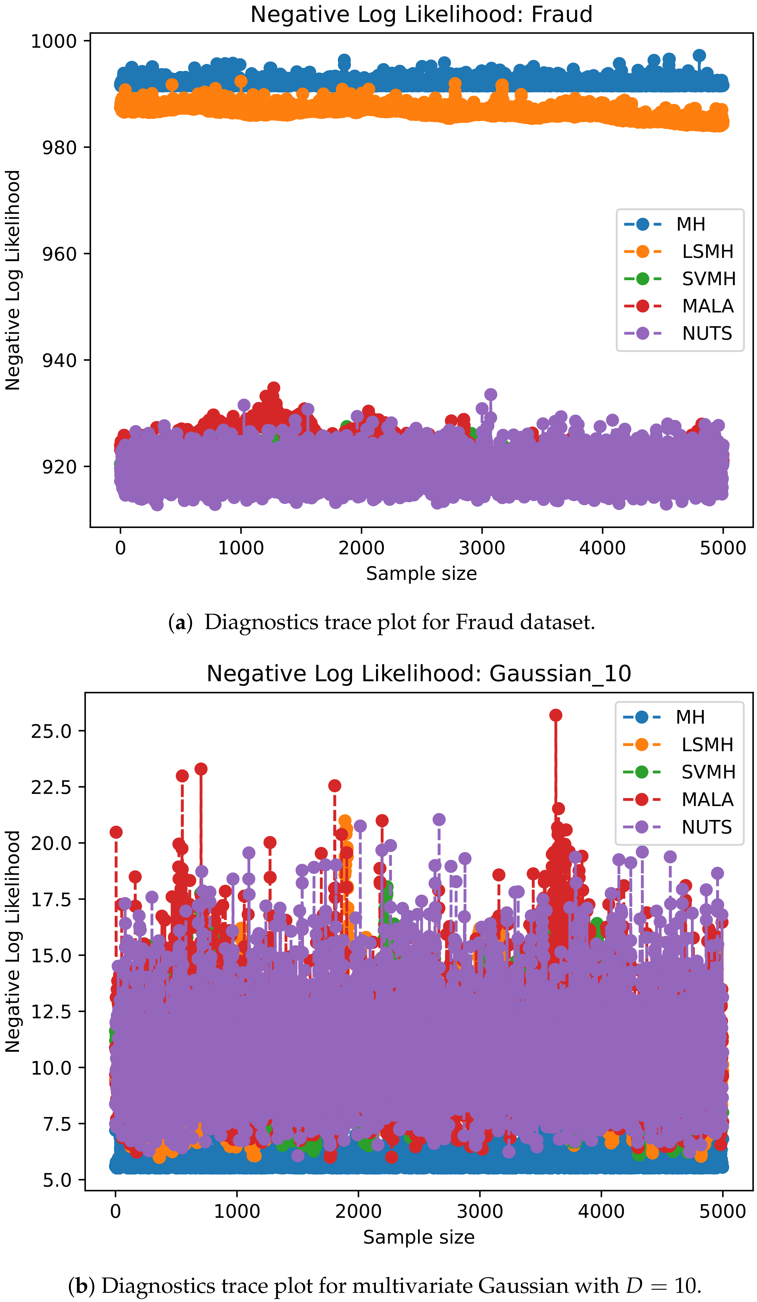
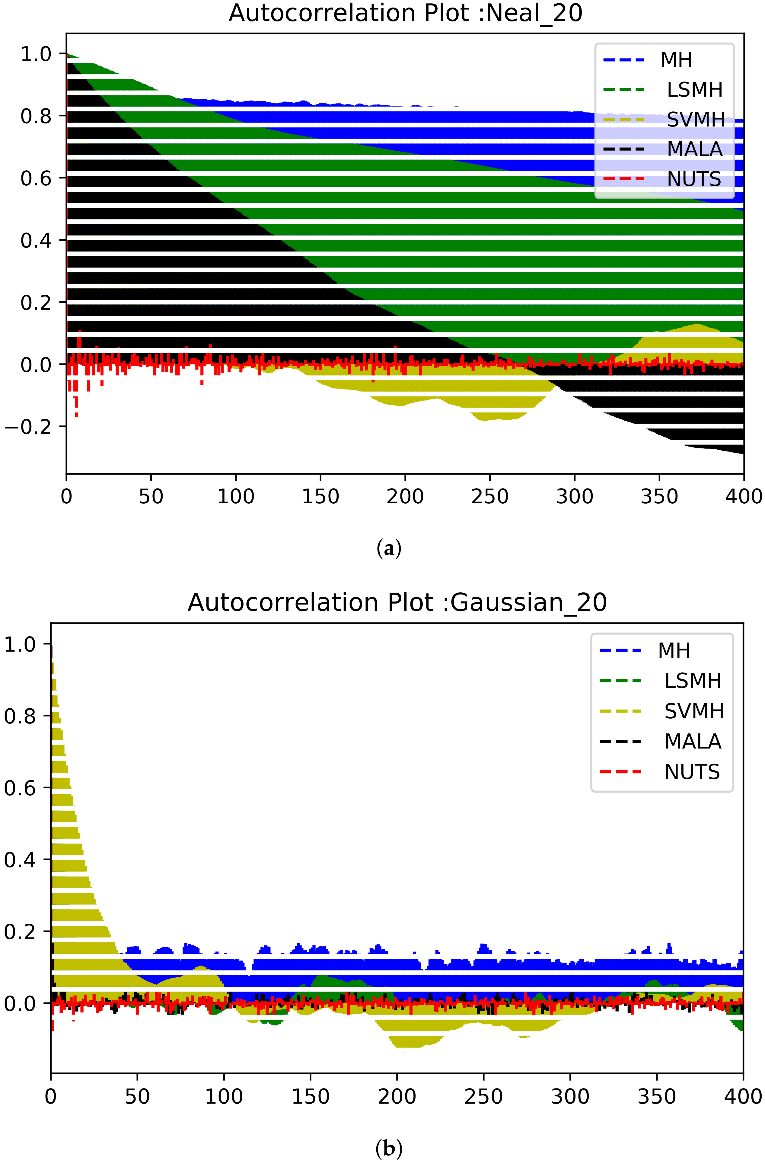
Figure 2 shows the diagnostic negative log-likelihood trace plots for each sampler across various targets. Figure 3 shows the autocorrelations produced by each MCMC method for the first dimension across various targets. Figure 4 shows the predictive performance of each of the sampling methods on the real world classification datasets modeled using BLR.

The first two rows in Figure 1 show the $m\mathbb{ESS}$ and $m\mathbb{ESS}$ normalised by execution time for the multivariate Gaussian distributions and Neal’s funnel used in the simulation study with increasing dimensionality D. The third and fourth row in Figure 1 show the $m\mathbb{ESS}$ and $m\mathbb{ESS}$ normalised by execution time for the financial market datasets modeled using jump diffusion processes, while rows five and six show the results for real world classification datasets modeled using Bayesian logistic regression. The results in Table 3 and Table 4 are the mean results over the thirty iterations for each algorithm.

The first couple rows of Figure 1 show that in all the values of D on both targets, SVMH and LSMH outperform MH in terms of effective sample sizes with SVMH and LSMH having similar effective sample sizes. When execution time is taken into consideration, SVMH outperforms LSMH and MH. The results also show that the NUTS algorithm outperforms all the MCMC methods on an effective sample size basis, while the MALA outperforms all the other MCMC methods on a normalised effective sample size basis.

Rows three to six in Figure 1 show that across all the real world datasets, SVMH and LSMH have similar effective sample sizes, with MH producing the smallest effective sample size. NUTS outperforms all the algorithms on an effective sample size basis. On a normalised effective sample size basis, SVMH outperforms all the algorithms on the jump diffusion datasets except for the USDZAR dataset. NUTS outperforms on the USDZAR dataset due to the lower kurtosis on this dataset as seen in Table 1. NUTS appears to perform poorly on the datasets that have a high kurtosis.

Figure 2 shows that the SVMH algorithm converges to the same level as NUTS on the majority of the datasets. On the other hand, the MH and LSMH algorithms converge to higher (i.e., less optimal) negative log-likelihoods. Figure 3 shows that NUTS produces the lowest autocorrelations on all the targets except on the jump-diffusion datasets. MH produces the highest autocorrelations on the majority of the targets. The autocorrelations on the SVMH algorithm are higher than NUTS and MALA but approach zero quicker than for MH across the targets considered. Note that these are auto correlations after the burn-in period.

Table 3 and Table 4 show that, as expected, MH produces the lowest execution time with SVMH being a close second. LSMH is slower than SVMH due to the computation of the Hessian matrix at each state. The NUTS algorithm has the highest execution time on the jump diffusion datasets.

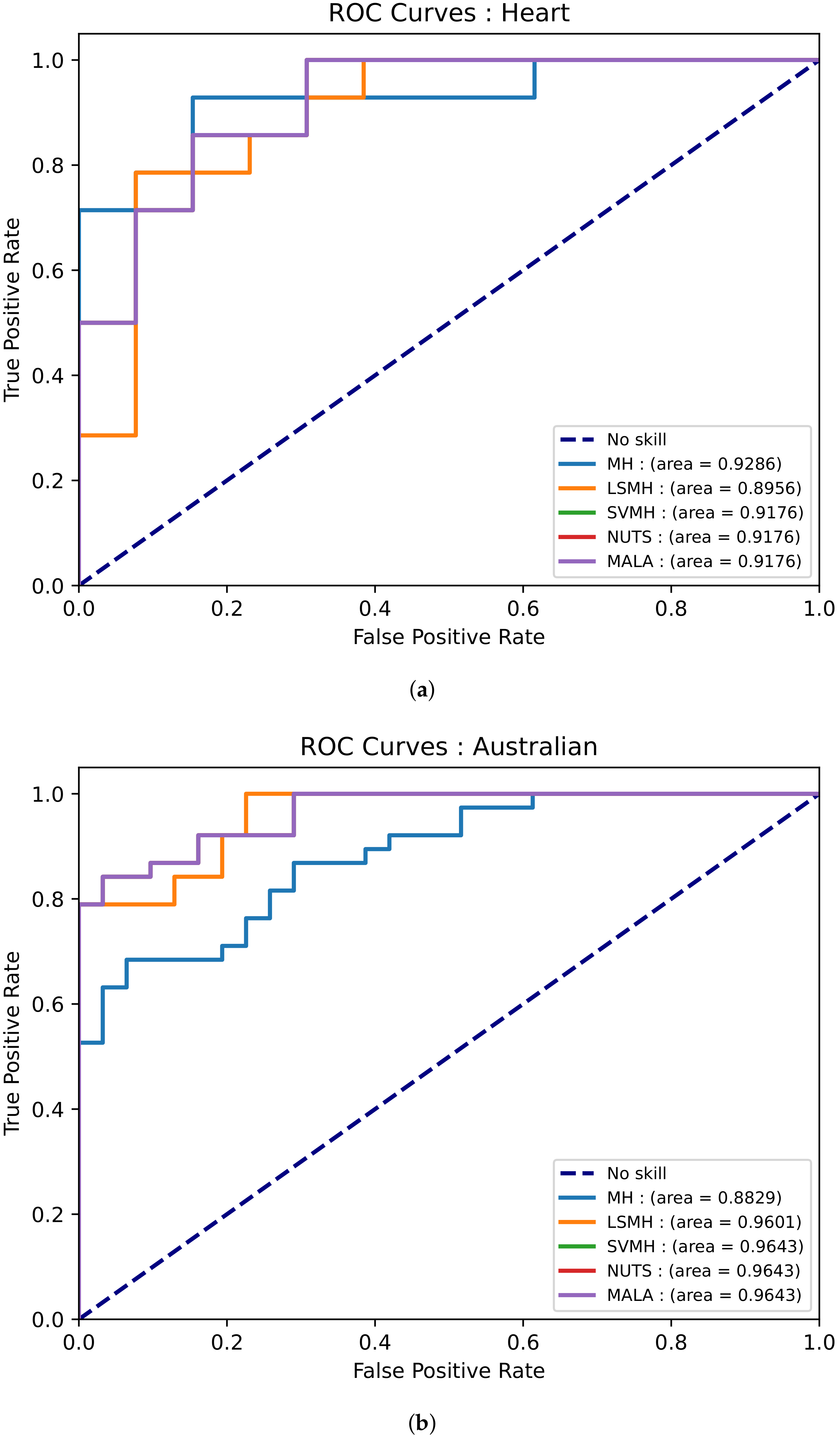
Table 3 and Table 4 as well as Figure 4 and Figure 5 show that, in terms of predictive performance using the negative log-likelihood on test data and AUC, the SVMH algorithm outperforms all the algorithms on the bulk of the real world datasets. Note that the SVMH method outperforms all the methods or has similar performance on a test negative log-likelihood basis on the logistic regression datasets. The results also show that the MH algorithm progressively becomes worse as the dimensions increase. The predictive performance of the LSMH algorithm is not stable as dimensions increase, with its performance at times being close to the MH algorithm.

It is worth noting that although LSMH and SVMH outperform the MH on several metrics, the LSMH and SVMH methods still produce low effective sample sizes compared with the required number of samples. This can potentially be improved by centering the proposal distribution at the current point plus first-order gradient—which should assist in guiding the exploration (and decrease the autocorrelations in the generated samples) as in Metropolis Adjusted Langevin Algorithm [4], and Hamiltonian Monte Carlo [3,14].

5. Conclusions

We introduce the stochastic volatility Metropolis–Hastings and locally scaled Metropolis–Hastings Markov chain Monte Carlo (MCMC) algorithms. We compare these methods with the vanilla Metropolis–Hastings algrouthm using a simulation study on multivariate Gaussian distributions and Neal’s funnel and real-world datasets modeled using jump diffusion processes and Bayesian logistic regression. The proposed methods are compared against the Metropolis–Hastings method, the Metropolis adjusted Langevin algorithm (MALA), and the No-U-Turn sampler.

Overall, the No-U-Turn sampler outperforms all the MCMC methods on an effective sample size basis. Stochastic Volatility Metropolis–Hastings (SVMH) and Locally Scaled Metropolis–Hastings produce higher effective sample sizes than Metropolis–Hastings, even after accounting for the execution time. In addition, SVMH outperforms all the methods in terms of predictive performance on the majority of the real world datasets. Furthermore, the SVMH method outperforms NUTS and MALA on the majority of the jump diffusion datasets on time normalised effective sample size basis. Given that SVMH does not add notable computational complexity to the Metropolis–Hastings algorithm, there seem to be trivial impediments to its use in place of Metropolis–Hastings in practice.

This work can be improved by examining the case where the scaling matrix in stochastic volatility Metropolis–Hastings is sampled from a Wishart distribution so that correlations between the different parameter dimensions are taken into account. An analysis to determine the optimal distribution for the scaling matrix could improve this paper. Constructing the stochastic volatility version of the Metropolis adjusted Langevin algorithm could also be of interest, significantly since Metropolis adjusted Langevin algorithm can use first-order gradient information to improve exploration of the target. Furthermore, we plan on including the calibration of jump diffusion with stochastic volatility characteristics using MCMC techniques in future work.

References

- Neal, R.M. Bayesian learning via stochastic dynamics. In Advances in Neural Information Processing Systems; MIT Press: Cambridge, MA, USA, 1993; pp. 475–482. [Google Scholar]
- Neal, R.M. MCMC Using Hamiltonian Dynamics. Available online: https://arxiv.org/pdf/1206.1901.pdf%20http://arxiv.org/abs/1206.1901 (accessed on 27 November 2021).
- Neal, R.M. Bayesian Learning for Neural Networks; Springer Science & Business Media: Berlin/Heidelberg, Germany, 2012; Volume 118. [Google Scholar]
- Girolami, M.; Calderhead, B. Riemann manifold langevin and hamiltonian monte carlo methods. J. R. Stat. Soc. Ser. B 2011, 73, 123–214. [Google Scholar] [CrossRef]
- Radivojević, T.; Akhmatskaya, E. Mix & Match Hamiltonian Monte Carlo. arXiv 2017, arXiv:1706.04032. [Google Scholar]
- Mongwe, W.T.; Mbuvha, R.; Marwala, T. Antithetic Magnetic and Shadow Hamiltonian Monte Carlo. IEEE Access 2021, 9, 49857–49867. [Google Scholar] [CrossRef]
- Mongwe, W.T.; Mbuvha, R.; Marwala, T. Antithetic Riemannian Manifold And Quantum-Inspired Hamiltonian Monte Carlo. arXiv 2021, arXiv:2107.02070. [Google Scholar]
- Mbuvha, R.; Marwala, T. Bayesian inference of COVID-19 spreading rates in South Africa. PLoS ONE 2020, 15, e0237126. [Google Scholar] [CrossRef] [PubMed]
- Mongwe, W.T.; Mbuvha, R.; Marwala, T. Magnetic Hamiltonian Monte Carlo With Partial Momentum Refreshment. IEEE Access 2021, 9, 108009–108016. [Google Scholar] [CrossRef]
- Mbuvha, R. Parameter Inference Using Probabilistic Techniques. Ph.D. Thesis, University Of Johannesburg, Johannesburg, South Africa, 2021. [Google Scholar]
- Mbuvha, R.; Mongwe, W.T.; Marwala, T. Separable Shadow Hamiltonian Hybrid Monte Carlo for Bayesian Neural Network Inference in wind speed forecasting. Energy AI 2021, 6, 100108. [Google Scholar] [CrossRef]
- Hastings, W.K. Monte Carlo sampling methods using Markov chains and their applications. Biometrika 1970, 57, 97–109. [Google Scholar] [CrossRef]
- Roberts, G.O.; Stramer, O. Langevin diffusions and Metropolis-Hastings algorithms. Methodol. Comput. Appl. Probab. 2002, 4, 337–357. [Google Scholar] [CrossRef]
- Duane, S.; Kennedy, A.D.; Pendleton, B.J.; Roweth, D. Hybrid monte carlo. Phys. Lett. B 1987, 195, 216–222. [Google Scholar] [CrossRef]
- Sweet, C.R.; Hampton, S.S.; Skeel, R.D.; Izaguirre, J.A. A separable shadow Hamiltonian hybrid Monte Carlo method. J. Chem. Phys. 2009, 131, 174106. [Google Scholar] [CrossRef] [PubMed] [Green Version]
- Mongwe, W.T.; Mbuvha, R.; Marwala, T. Adaptively Setting the Path Length for Separable Shadow Hamiltonian Hybrid Monte Carlo. IEEE Access 2021, 9, 138598–138607. [Google Scholar] [CrossRef]
- Mongwe, W.T.; Mbuvha, R.; Marwala, T. Utilising Partial Momentum Refreshment in Separable Shadow Hamiltonian Hybrid Monte Carlo. IEEE Access 2021, 9, 151235–151244. [Google Scholar] [CrossRef]
- Tripuraneni, N.; Rowland, M.; Ghahramani, Z.; Turner, R. Magnetic hamiltonian monte carlo. In Proceedings of the International Conference on Machine Learning (PMLR), Sydney, Australia, 6–11 August 2017; pp. 3453–3461. [Google Scholar]
- Mongwe, W.T.; Mbuvha, R.; Marwala, T. Quantum-Inspired Magnetic Hamiltonian Monte Carlo. PLoS ONE 2021, 16, e0258277. [Google Scholar] [CrossRef] [PubMed]
- Mongwe, W.T.; Mbuvha, R.; Marwala, T. Adaptive Magnetic Hamiltonian Monte Carlo. IEEE Access 2021, 9, 152993–153003. [Google Scholar] [CrossRef]
- Yang, J.; Roberts, G.O.; Rosenthal, J.S. Optimal scaling of random-walk metropolis algorithms on general target distributions. Stoch. Process. Their Appl. 2020, 130, 6094–6132. [Google Scholar] [CrossRef]
- Roberts, G.O.; Rosenthal, J.S. Optimal scaling for various Metropolis-Hastings algorithms. Stat. Sci. 2001, 16, 351–367. [Google Scholar] [CrossRef]
- Vogrinc, J.; Kendall, W.S. Counterexamples for optimal scaling of Metropolis–Hastings chains with rough target densities. Ann. Appl. Probab. 2021, 31, 972–1019. [Google Scholar] [CrossRef]
- Dahlin, J.; Lindsten, F.; Schön, T.B. Particle Metropolis–Hastings using gradient and Hessian information. Stat. Comput. 2015, 25, 81–92. [Google Scholar] [CrossRef] [Green Version]
- Liu, Z.; Zhang, Z. Quantum-Inspired Hamiltonian Monte Carlo for Bayesian Sampling. arXiv 2019, arXiv:1912.01937. [Google Scholar]
- Merton, R.C. Option pricing when underlying stock returns are discontinuous. J. Financ. Econ. 1976, 3, 125–144. [Google Scholar] [CrossRef] [Green Version]
- Levy, D.; Hoffman, M.D.; Sohl-Dickstein, J. Generalizing hamiltonian monte carlo with neural networks. arXiv 2017, arXiv:1711.09268. [Google Scholar]
- Yan, G.; Hanson, F.B. Option pricing for a stochastic-volatility jump-diffusion model with log-uniform jump-amplitudes. In Proceedings of the 2006 American Control Conference, Minneapolis, MN, USA, 14–16 June 2006; IEEE: Piscataway, NJ, USA, 2006; p. 6. [Google Scholar]
- Brooks, S.; Gelman, A.; Jones, G.; Meng, X.L. Handbook of Markov Chain Monte Carlo; CRC Press: Boca Raton, FL, USA, 2011. [Google Scholar]
- Betancourt, M. A conceptual introduction to Hamiltonian Monte Carlo. arXiv 2017, arXiv:1701.02434. [Google Scholar]
- Gu, M.; Sun, S. Neural Langevin Dynamical Sampling. IEEE Access 2020, 8, 31595–31605. [Google Scholar] [CrossRef]
- Hoffman, M.D.; Gelman, A. The No-U-turn sampler: Adaptively setting path lengths in Hamiltonian Monte Carlo. J. Mach. Learn. Res. 2014, 15, 1593–1623. [Google Scholar]
- Afshar, H.M.; Oliveira, R.; Cripps, S. Non-Volume Preserving Hamiltonian Monte Carlo and No-U-TurnSamplers. In Proceedings of the International Conference on Artificial Intelligence and Statistics (PMLR), Virtual Conference, 13–15 April 2021; pp. 1675–1683. [Google Scholar]
- Betancourt, M.J. Generalizing the no-U-turn sampler to Riemannian manifolds. arXiv 2013, arXiv:1304.1920. [Google Scholar]
- Betancourt, M. A general metric for Riemannian manifold Hamiltonian Monte Carlo. In Proceedings of the International Conference on Geometric Science of Information, Paris, France, 28–30 August 2013; Springer: Berlin/Heidelberg, Germany, 2013; pp. 327–334. [Google Scholar]
- Vats, D.; Flegal, J.M.; Jones, G.L. Multivariate output analysis for Markov chain Monte Carlo. Biometrika 2019, 106, 321–337. Available online: http://xxx.lanl.gov/abs/https://academic.oup.com/biomet/article-pdf/106/2/321/28575440/asz002.pdf (accessed on 27 November 2021). [CrossRef] [Green Version]
- Hoffman, M.D.; Gelman, A. The No-U-Turn Sampler: Adaptively Setting Path Lengths in Hamiltonian Monte Carlo. arXiv 2011, arXiv:1111.4246. [Google Scholar]
- Andrieu, C.; Thoms, J. A tutorial on adaptive MCMC. Stat. Comput. 2008, 18, 343–373. [Google Scholar] [CrossRef]
- Neal, R.M. Slice sampling. Ann. Stat. 2003, 31, 705–741. [Google Scholar] [CrossRef]
- Betancourt, M.; Girolami, M. Hamiltonian Monte Carlo for hierarchical models. In Current Trends in Bayesian Methodology with Applications; CRC Press: Boca Raton, FL, USA, 2015; Volume 79, pp. 2–4. [Google Scholar]
- Heide, C.; Roosta, F.; Hodgkinson, L.; Kroese, D. Shadow Manifold Hamiltonian Monte Carlo. In Proceedings of the International Conference on Artificial Intelligence and Statistics (PMLR), Virtual Conference, 13–15 April 2021; pp. 1477–1485. [Google Scholar]
- Cont, R. Empirical properties of asset returns: Stylized facts and statistical issues. Quant. Financ. 2001, 1, 223–236. [Google Scholar] [CrossRef]
- Mongwe, W.T. Analysis of Equity and Interest Rate Returns in South Africa under the Context of Jump Diffusion Processes. Master’s Thesis, University of Cape Town, Cape Town, South Africa, 2015. [Google Scholar]
- Aït-Sahalia, Y.; Li, C.; Li, C.X. Closed-form implied volatility surfaces for stochastic volatility models with jumps. J. Econom. 2021, 222, 364–392. [Google Scholar] [CrossRef]
- Alghalith, M. Pricing options under simultaneous stochastic volatility and jumps: A simple closed-form formula without numerical/computational methods. Phys. A Stat. Mech. Its Appl. 2020, 540, 123100. [Google Scholar] [CrossRef]
- Van der Stoep, A.W.; Grzelak, L.A.; Oosterlee, C.W. The Heston stochastic-local volatility model: Efficient Monte Carlo simulation. Int. J. Theor. Appl. Financ. 2014, 17, 1450045. [Google Scholar] [CrossRef] [Green Version]
- Press, S.J. A compound events model for security prices. J. Bus. 1967, 40, 317–335. [Google Scholar] [CrossRef]
- Google-Finance. Google Finance. Available online: https://www.google.com/finance/ (accessed on 15 August 2021).
- Michie, D.; Spiegelhalter, D.J.; Taylor, C.C.; Campbell, J. (Eds.) Machine Learning, Neural and Statistical Classification; Ellis Horwood: New York, NY, USA, 1995. [Google Scholar]
- Mongwe, W.T.; Malan, K.M. A Survey of Automated Financial Statement Fraud Detection with Relevance to the South African Context. South Afr. Comput. J. 2020, 32, 74–112. [Google Scholar] [CrossRef]
- Mongwe, W.T.; Malan, K.M. The Efficacy of Financial Ratios for Fraud Detection Using Self Organising Maps. In Proceedings of the 2020 IEEE Symposium Series on Computational Intelligence (SSCI), Canberra, Australia, 1–4 December 2020; IEEE: Piscataway, NJ, USA, 2020; pp. 1100–1106. [Google Scholar]
Figure 1.
Inference results across each dataset over thirty iterations of each algorithm. The first row is the effective sample size while the second row is the time-normalised effective sample size for each dataset.
Figure 2.
Negative log-likelihood diagnostic trace plots for various targets. These are traces plots from a single run of the MCMC chain. (a) Diagnostic negative log-likelihood trace plots for the Fraud dataset and (b) Diagnostic negative log-likelihood trace plots for the multivariate Gaussian with . The other targets produce similar convergence behavior.
Figure 3.
Autocorrelation plots for the first dimension across the various targets. These are autocorrelations from a single run of the MCMC chain. (a) Autocorrelation plot for the first dimension on the Neal funnel for and (b) Autocorrelation plot for the first dimension on the multivariate Gaussian with .
Figure 4.
Predictive performance for all the sampling methods on the real world classification datasets. The results were averaged over thirty runs of each algorithm. (a) ROC curves for the Heart dataset and (b) ROC curves for Australian credit dataset.
Figure 5.
Predictive performance for all the sampling methods on the real world classification datasets. The results were averaged over thirty runs of each algorithm. (a) ROC curves for the Fraud dataset and (b) ROC curves for German dataset.