MapReduce Algorithm for Location Recommendation by Using Area Skyline Query

Abstract

Location recommendation is essential for various map-based mobile applications. However, it is not easy to generate location-based recommendations with the changing contexts and locations of mobile users. Skyline operation is one of the most well-established techniques for location-based services. Our previous work proposed a new query method, called “area skyline query”, to select areas in a map. However, it is not efficient for large-scale data. In this paper, we propose a parallel algorithm for processing the area skyline using MapReduce. Intensive experiments on both synthetic and real data confirm that our proposed algorithm is sufficiently efficient for large-scale data.

1. Introduction

With the development of mobile device technologies and GPS systems, various map-based mobile applications such as Google Maps and Apple Maps have become popular in recent years. Since the limitations of display size and processing power of mobile devices, we need to recommend the appropriate information such as good locations for users. However, it is difficult to generate location-based recommendations in mobile devices with the changing contexts and locations of mobile users.

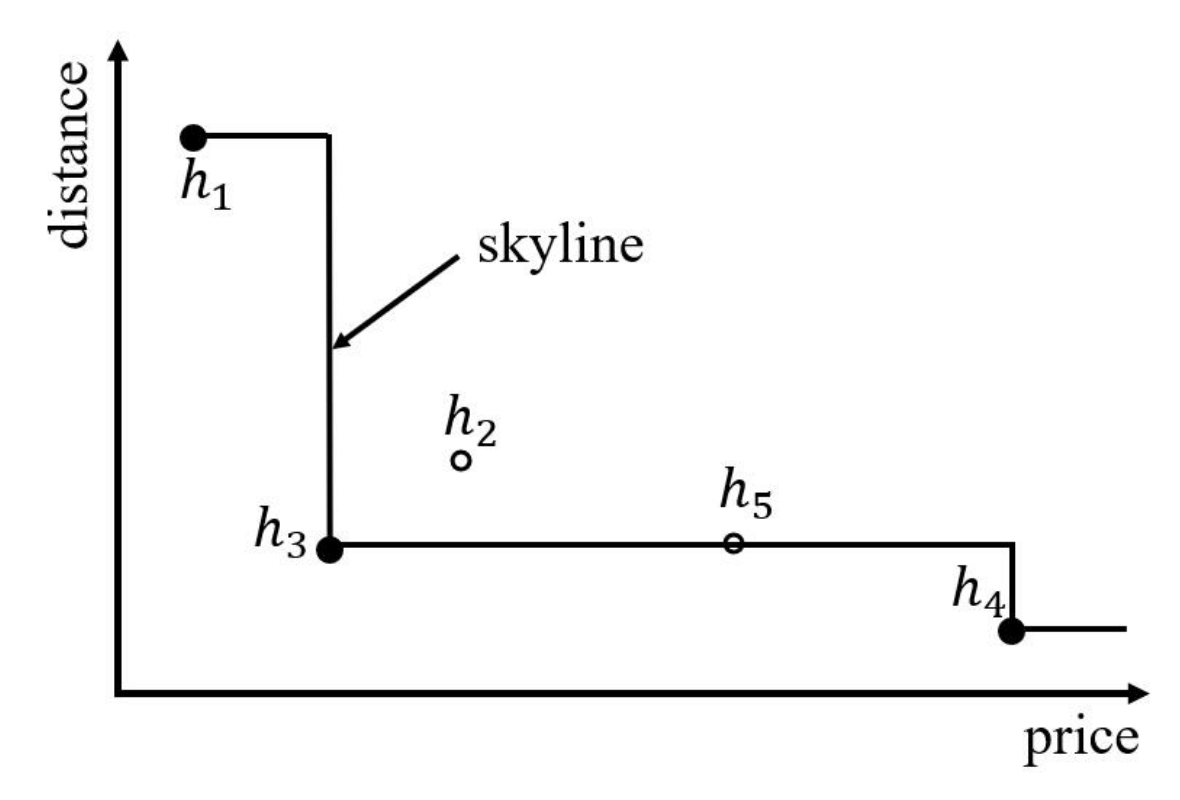
1.1. Skyline Query

Skyline operation [1] is a well-established technique which can select interesting items from a large database. Let $\mathbf{D}$ be a $\mathit{d}$-dimensional database. Given a set of points {$p_1,p_2,\dots ,p_n$}, a point $p_i$ is said to dominate another point $p_j(i\ne j)$ if $p_i$ is not worse than $p_j$ in any of the $\mathit{d}$-dimensions and $p_i$ is better than $p_j$ in at least one of the d-dimensions. Then, the skyline query returns a small number of points, each of which is not dominated by other points in $\mathbf{D}$. The excellent ability in filtering the uninteresting objects makes the skyline query a good candidate for the location recommendation problem.

In general, a good location should be close to preferable facilities such as shopping malls, sightseeing spots, bus/train stations, etc. and be far away from unpreferable facilities such as factories, open landfills, etc.

Table 1. A Hotel Example.

ID	Price	Distance
$h_1$	3	8
$h_2$	5	4
$h_3$	4	3
$h_4$	9	2
$h_5$	7	3

and Figure 1 demonstrate an example for location selection by using the skyline queries. Recommenders aim to find a low-cost hotel with a shorter distance to the bus/train station. However, hotels with convenient transportation are usually relatively higher for the room prices. For example, there are five candidate hotels {$h_1,h_2,\dots ,h_5$} in Table 1. Each $h_i$ has two-dimensions, which are the room price and the distance to the nearest bus/train station. $h_1$ has the lowest room price but the longest distance from the bus/train station. In contrast, the most convenient $h_4$ has the highest room price. Figure 1 shows that the hotel $h_2$ and the hotel $h_5$ are dominated by $h_3$, while $h_1,h_3$ and $h_4$ are not dominated each other. Therefore, the skyline objects are {$h_1,h_3,h_4$}.

Skyline queries have attracted much attention recently since the queries can be formulated as an intuitive process. There exist many skyline query algorithms, which are recorded in [2,3,4]. However, most of the existing skyline queries are zero-dimensional data. Since locations are typical two-dimensional data, the general skyline queries cannot solve the spatial relationships between objects. Based on such consideration, we consider using the spatial skyline queries to solve such problem.

1.2. Spatial Skyline Query

Figure 2 and

Table 2. Distance Table.

Point	$\mathit{F}{1}^{+}$	$\mathit{F}{2}^{+}$	$\mathit{F}{3}^{-}$
$p_1$	3	5	−10
$p_2$	4	9	−7
$p_3$	8	1	−8

demonstrate an example of spatial skyline queries. In Figure 2, we use square symbols, triangle symbols and star symbols to indicate the location of facilities. Notice that “+” mark on the facility symbol represent preferable facilities such as bus/train stations, while “−” mark on the facility symbol for unpreferable ones such as open landfills. We represent the star symbols and triangle symbols as the preferable facilities, while the square symbols for unpreferable facilities. The star symbols and the triangle symbols are denoted as $F{1}^{+}=\{f{1}_1^{+},f{1}_2^{+},f{1}_3^{+}\}$ and $F{2}^{+}=\{f{2}_1^{+},f{2}_2^{+},f{2}_3^{+}\}$, while the square symbols are denoted as $F{3}^{-}=\{f{3}_1^{-},f{3}_2^{-},f{3}_3^{-}\}$.

In Table 2, there are three candidate points $p_1,p_2,p_3$. The values represent the distance of the candidate point $p_i(i=1,2,3)$ to the nearest facilities. For example, the nearest facilities of the candidate point $p_1$ are $f{1}_1^{+},f{2}_1^{+},f{3}_3^{-}$ for facility type $F1,F2$ and $F3$. The distances are $3,5$ and 10 respectively. We assume that the smaller value is better, so that we multiply -1 to each distance value of unpreferable facilities $F^{-}$. In this example, point $p_1$ dominates point $p_2$, since the values of $F{1}^{+},F{2}^{+}$ and $F{3}^{-}$ of point $p_1$ are smaller than the values of point $p_2$. $p_3$ is not dominated by $p_1$ and $p_2$, since $p_3$ is closer to $F{2}^{+}$ than $p_1,p_2$ but farther to $F{3}^{-}$ than $p_2$. So the skyline objects are $p_1$ and $p_3$. In general, we can address the spatial skyline problem by conventional skyline queries after calculating the data table such as Table 2.

However, in some real-world scenarios, the candidate points like $p_1,\dots ,p_n$ are not given for the location recommendation problem. In this situation, we need to find a two-dimensional area with more preferable facilities around it and away from the unpreferable facilities. To address such problem, we proposed the “Area Skyline Query” in our previous work [5], which is a new selection method of areas in a map.

1.3. Area Skyline Query

Assume that A is a square region in a map. Let $F=\{F1,F2,\dots ,Fm\}$ be a set of facility types. A traveler wants to find an excellent touristic place in a map where is close to some preferable facilities and is far from some unpreferable facilities. In this scenario, we define area skyline and area dominance as follows:

Definition 1. 

(Area Skyline) We divide a square region A into $n\times n$ grids $G=\{g_{1,1},\dots ,g_{n,n}\}$. A grid $g_i$ is said to be in skyline if there is no other grid $g_j(i\ne j)$ in a map such that the distance of $g_j$ to the nearest preferable facilities are smaller than that of $g_i$ and the distance to the nearest unpreferable facilities are larger than that of $g_i$.

Definition 2. 

(Area Dominance) If there exists such gird $g_j$, we say that $g_i$ is dominated by $g_j$ or $g_j$ dominates $g_i$.

Figure 3 demonstrates an example of area skyline queries. We compute the area skyline objects by the algorithm proposed in [5] which we call it grid-based area skyline (GASKY). In the map, the area skyline objects are the shaded grids which are not dominated by each other. In other words, the shaded grids are closer to the preferable facilities and are farther from the unpreferable facilities than the unshaded grids. The unshaded grids are the dominated grids which can be eliminated from candidates.

We use GASKY algorithm as the selection method of areas in a map. However, the time complexity of the GASKY algorithm is worse than those conventional skyline queries. Furthermore, the average processing time increases linearly with the growth of facilities. In this paper, we propose a novel algorithm to resolve the poor performance problem of GASKY in the MapReduce framework, which we call “MRGASKY”.

The main contributions of this paper are as follows:

• We develop MapReduce-based area skyline query computation, which is a distributed algorithm to address the poor performance problem for the grid-based area skyline queries.
• We propose an efficient algorithm of the MapReduce-based computation.
• We conduct an extensive performance evaluation, which shows the high efficiency and scalability of our proposed algorithm.

The remainder of the paper is organized as follows. Section 2 surveys the related works. In Section 3, we formally define the problem and propose our efficient MRGASKY algorithm. Section 4 demonstrate the experimental validation of our proposed algorithm. Finally, Section 5 concludes the paper.

2. Related Works

2.1. Skyline Query

Studies on skyline computation have a long history. Brozsonyi et al. [1] first introduced skyline queries in large database applications and proposed Block Nested-Loop (BNL), Divide-and-Conquer (D&C) and B-tree based algorithms. Chomicki et al. [2] proposed an efficient skyline computation algorithm, Sort-Filter-Skyline (SFS), which improved BNL by presorting. Tan et al. [3] proposed two progressive algorithms, called Bitmap and Index, to improve the computation of skyline queries. Currently, Brach and Bound Skyline (BBS) has been the most effective algorithm, proposed by Papadias et al. [4], which is a progressive algorithm based on the Best First Nearest Neighbor (BFNN) algorithm. Due to the increase of the data dimensionality, many research are proposed to address the dimensionality problem of skyline queries such as skyline frequency [6], k-dominant skyline [7] and k-representative skylines [8]. These research works focused on the non-spatial database. However, spatial relationships between data points are playing an important role in our real life.

2.2. Spatial Skyline Query

Sharifzadeh et al. [9] first addressed the problem of spatial skyline queries. They proposed two algorithms for static query points said $B^2{S}^2$ and $V{S}^2$, and one algorithm for dynamic query points said $VC{S}^2$ which exploited the pattern of change in query points to avoid unnecessary re-computation of the skyline.

There exists other literature relating to the spatial skyline problem [10,11,12,13]. Kodama et al. [10] considered that the candidates should be close to the facilities. In [11], Kodama et al. considered non-spatial preferences, facility types, which had an impact on spatial skyline computation. Sometimes the retrieved data points should be far from those unpreferable facilities. Based on this consideration, You et al. [12] first studied TFSS algorithm and proposed a new progressive method, called Branch-and-Bound Farthest Spatial Skyline (BBFS) to compute the farthest spatial skyline queries. The results outperformed TFSS by exploiting spatial locality. In [13], Lin et al. considered that the retrieved data objects not only should be close to preferable facilities but also should be far from unpreferable facilities by using EFFN algorithm.

In some cases, the candidate points may not exist in the real world. Annisa et al. [14] proposed Unfixed-Shape Areas Skyline (UASKY) to make location recommendations without candidate points. Specifically, they used a Voronoi Diagram to divide a given region into disjoint subregions. For each subregion, they executed the previous process again by other facility types. Finally, they computed the distance to the nearest surrounding facilities in each sub-subregion. In [5], Annisa et al. proposed another location-based skyline query, called Grid-based Area Skyline (GASKY), which outperformed UASKY by partition a given region into $n\times n$ grids.

Most of the existing research for skyline computations rely on some centralized indexing structures. However, with the development of Internet technology, the amount of data increases exponentially. The centralized indexing structures cannot work well.

2.3. MapReduce Based Skyline Computation

In recent year, distributed skyline computations for big data has received more attention. Hose et al. [15] provided a good survey of skyline processing in highly distributed environments. MapReduce is a programming model and an associated implementation for processing a massive volume of data. It is widely used for computing skyline in recent years [16,17,18,19,20].

Three MapReduce based algorithms for skyline query processing, MR-BNL, MR-SFS, and MR-Bitmap, are proposed by Zhang et al. [16]. Experiments illustrated the effectiveness and efficiency of these algorithms compared to conventional skyline algorithms. Chen et al. [17] proposed a new MapReduce skyline method to compute skyline queries. The new angular partitioning of the data space significantly reduced the processing time. Papadias et al. [18] developed a MapReduce-based computation algorithm to implement k-dominant skyline query processing. In [19], Wu et al. proposed a novel distributed skyline query processing algorithm (DSL) that discovers skyline points progressively based on the grid structure. Wang et al. [20] adapted skyline computation to the MapReduce framework and they recursively divided the dimensions of data into some parts on a grid-based partitioning scheme. Unfortunately, few works implemented the spatial skyline queries in such distributed way. In this paper, We develop MapReduce-based area skyline query computation, which is a distributed algorithm for spatial skyline queries.

3. MapReduce-Based Area Skyline

We first divide a given region A into $n\times n$ grids on average by using a grid structure. To distinguish the grids, we assign IDs to all the grids from bottom-left $g_{1,1}$ to top-right $g_{n,n}$ (see Figure 3). Next, for each row, we calculate the distance of each grid to each type of facilities in the Map function. Then, we calculate the distance for each column in Reduce function. Using the distances for each type of facilities, we retrieve non-dominated grids. To simplify the problem, we assume that the distance between a facility and a grid is approximate to the distance of the center of the two grids when the length of the grid is small enough.

MRGASKY Algorithm

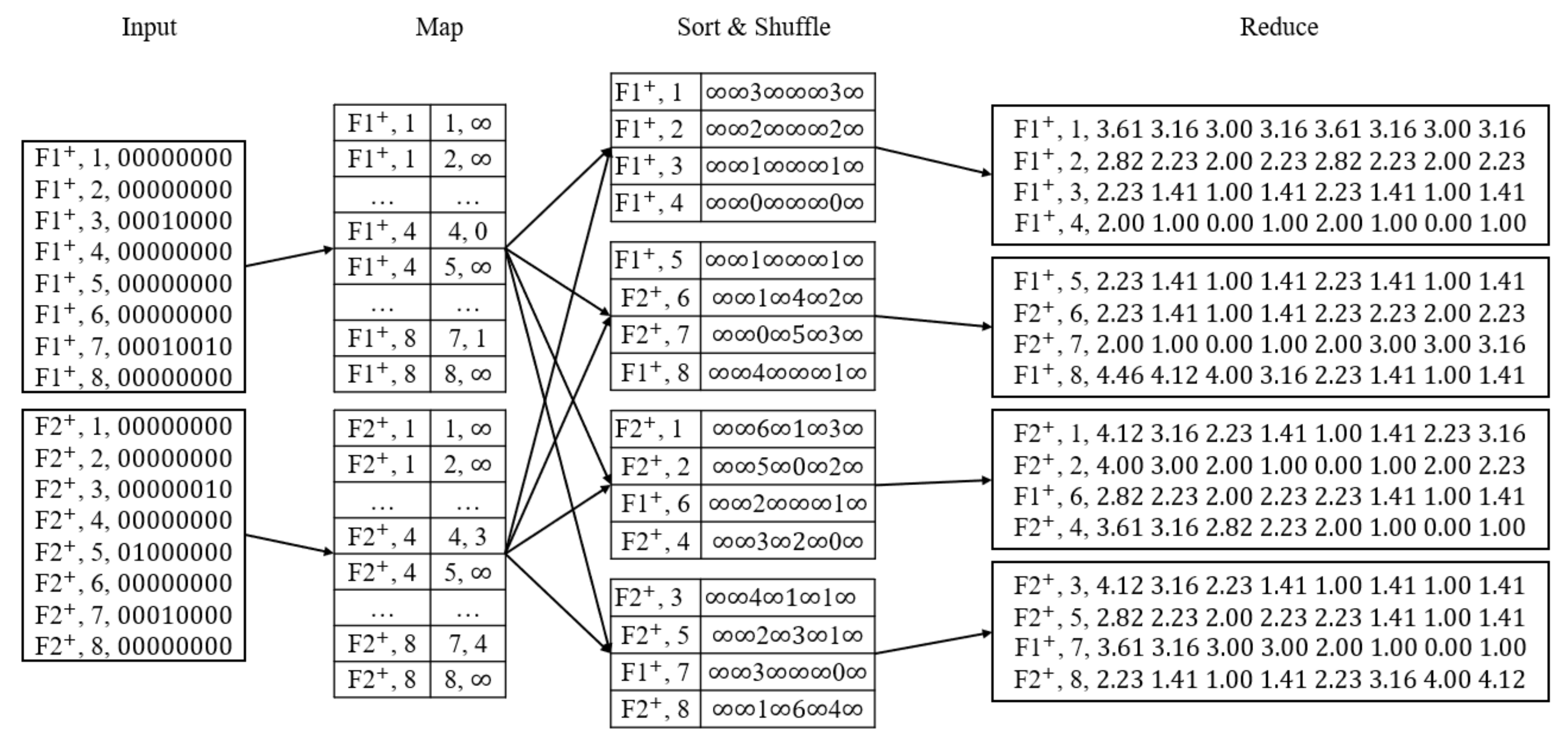
Step 1 

Map function mainly calculates the distance to the closest facilities of each type in the same row.

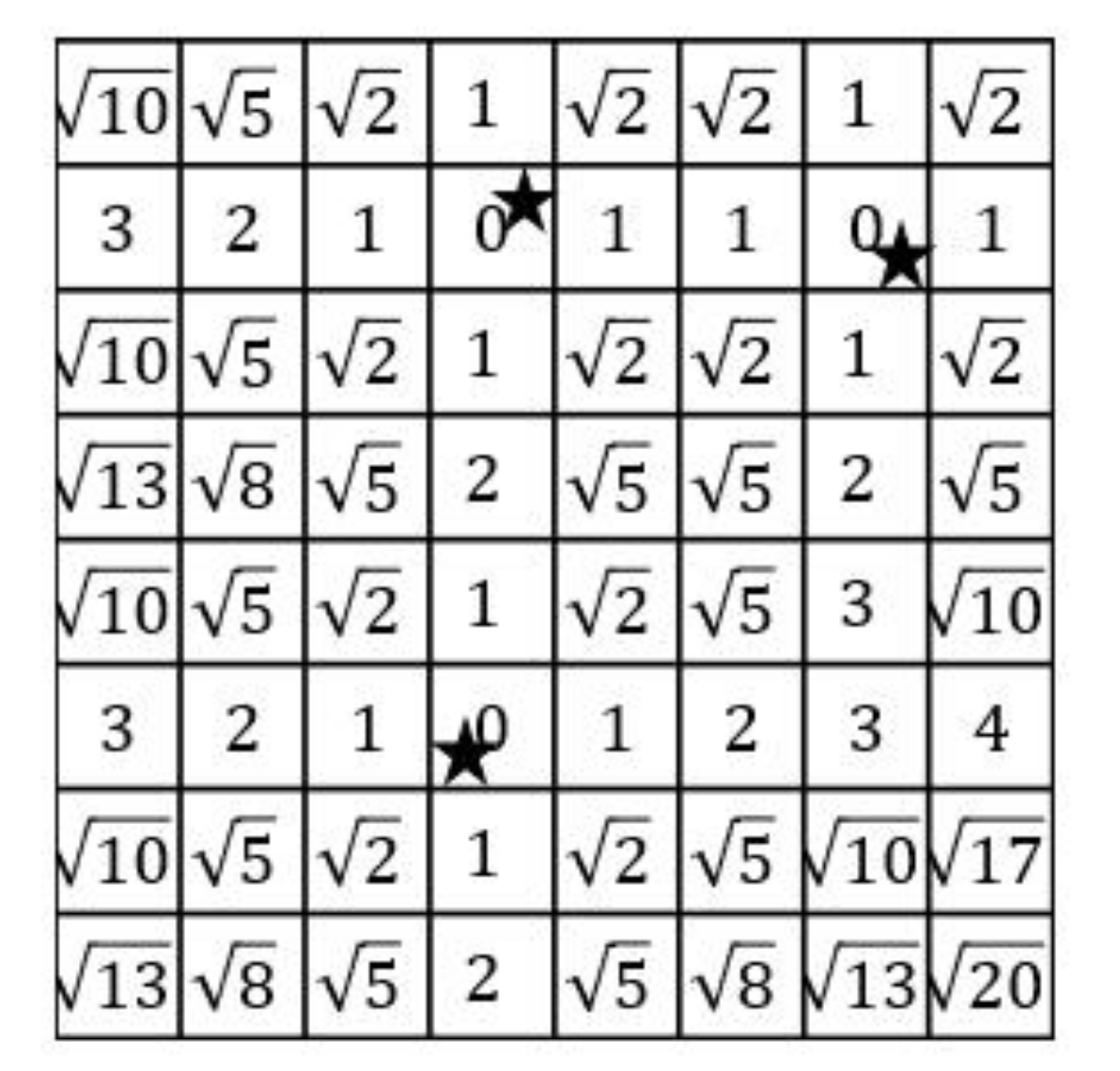
Step 1.1 

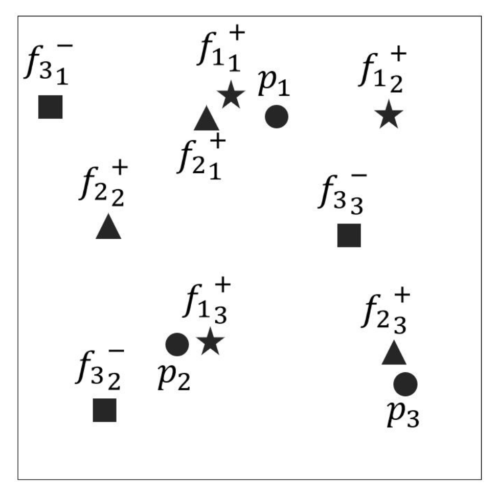
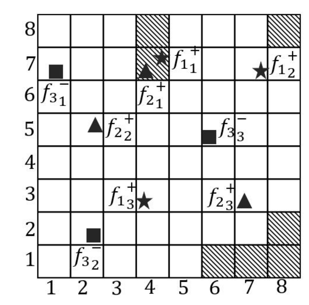
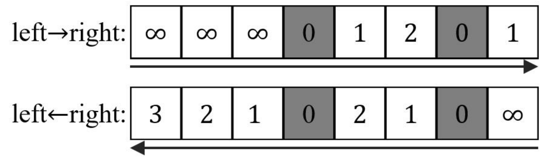
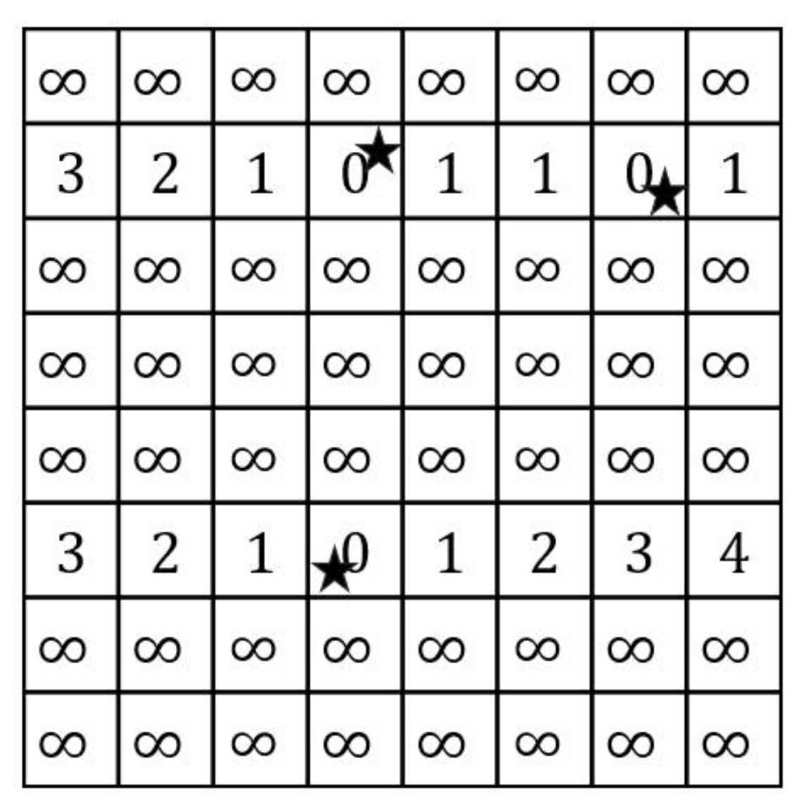
A map is firstly separated to n rows. For each row, the Map function reads the grids from both sides to calculate the distance between grids and facilities. We assume that the initial values of all grids are infinite before facilities are encountered. When facilities are encountered, the values of the grids are considered as 0. Then, the value of the next grid is updated based on the former grid plus one until the next facility is encountered. An example of 7th row of Figure 3 demonstrates in Figure 4. The shaded grids are the facilities of $F{1}^{+}$. The values of these shaded grids are 0. From left to right side, the values of the 5th, 6th and 8th grids are updated to 1, 2 and 1. Similarly, we can also compute the values from right to left side.

Step 1.2 

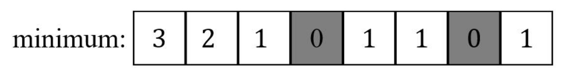
After calculating the values from both sides, we select the minimum value of every grid as the output of the Map function, as illustrated in Figure 5.

Algorithm 1 shows the algorithm of Map function. The map is stored in Hadoop distributed file system (HDFS) which is formed as a binary image. Specifically, for a binary image of size $n\times n$, $m_{i,j}(1\le i,j\le n)$ is an array which includes every type of facilities in the grid of ith row and jth column. $m_{i,j}\left[k\right](k\le m)$ is the kth element of array $m_{i,j}$, where m is the total number of facility types. $m_{i,j}\left[k\right]=1$ represents the facility of kth type is inside the grid $g_{i,j}$ and $m_{i,j}\left[k\right]=0$ represents that there are no facilities of kth facility type inside grid $g_{i,j}$. The Map output are the $key-value$ pairs. The $key$ is the column ID j and row ID i of grid $g_{i,j}$, and the $value$ is the distance we calculated in step 1.

Algorithm 1 Map Function for Step 1 Process

Input: A binary image Output: (key, value)=(type x-coordinate of grids. y-coordinate of grids, distance) 1: for each line in HDFS do 2:     calculate the Euclidean Distance from left to right: $dis{t}_{left\to right}$ 3:     calculate the Euclidean Distance from right to left: $dis{t}_{left\leftarrow right}$ 4: end for 5: for each grid in the same row do 6:     $dis{t}_{min}=min(dis{t}_{left\to right},dis{t}_{left\leftarrow right})$ 7: end for

We show the results of $key-value$ pairs after calculating step 1 process of facility type $F{1}^{+}$ in Figure 6.

Step 2 

Again, we calculate the distance of every grid to the nearest facilities in the same column in Reduce function.

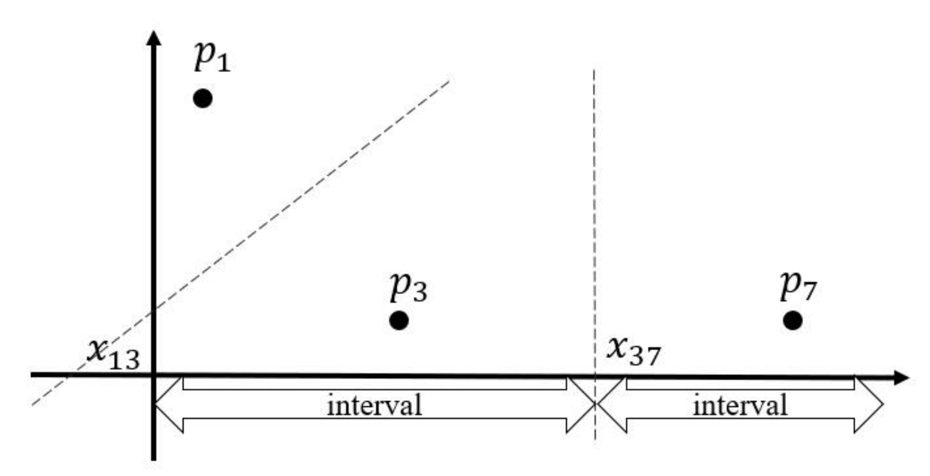
Step 2.1 

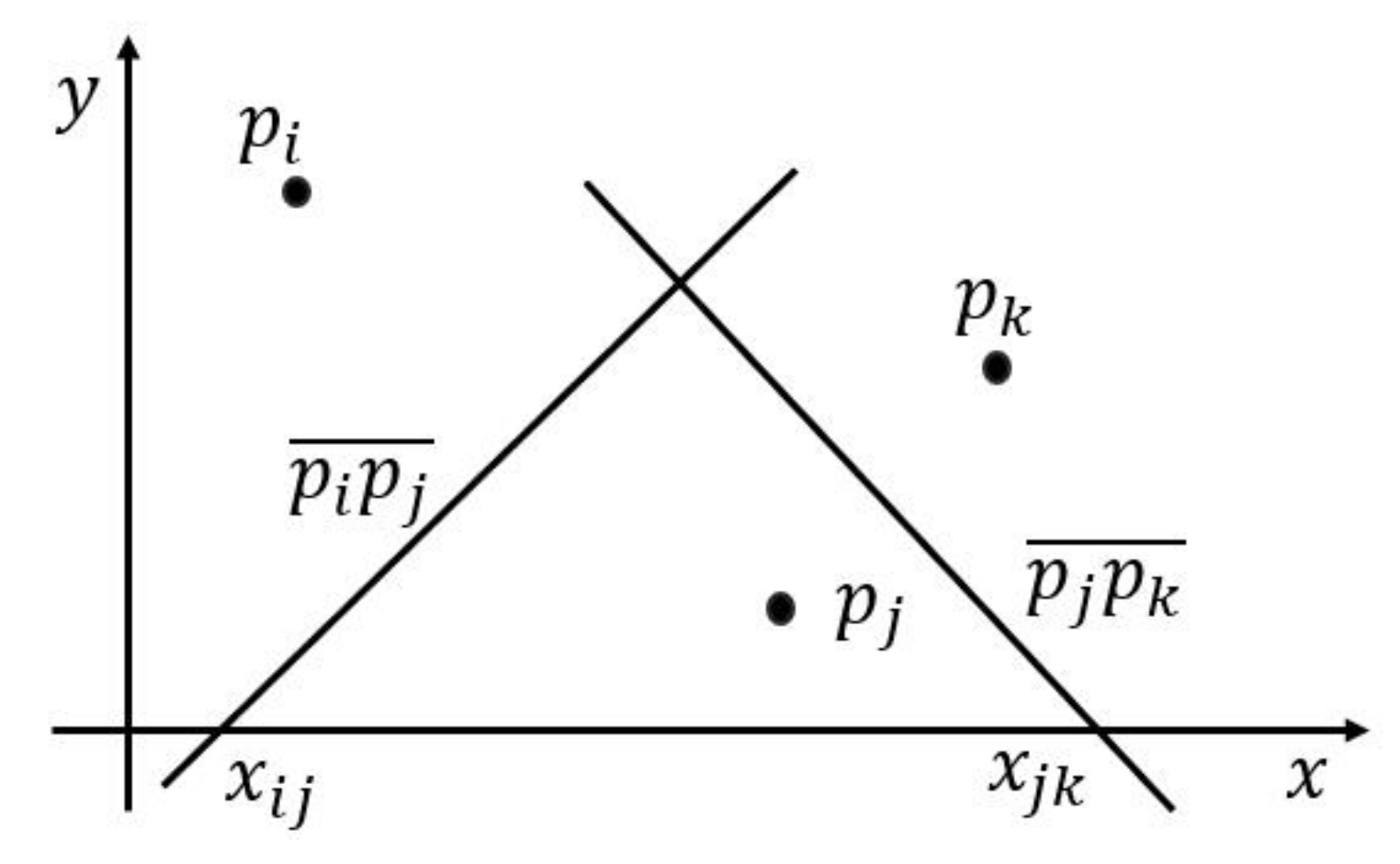
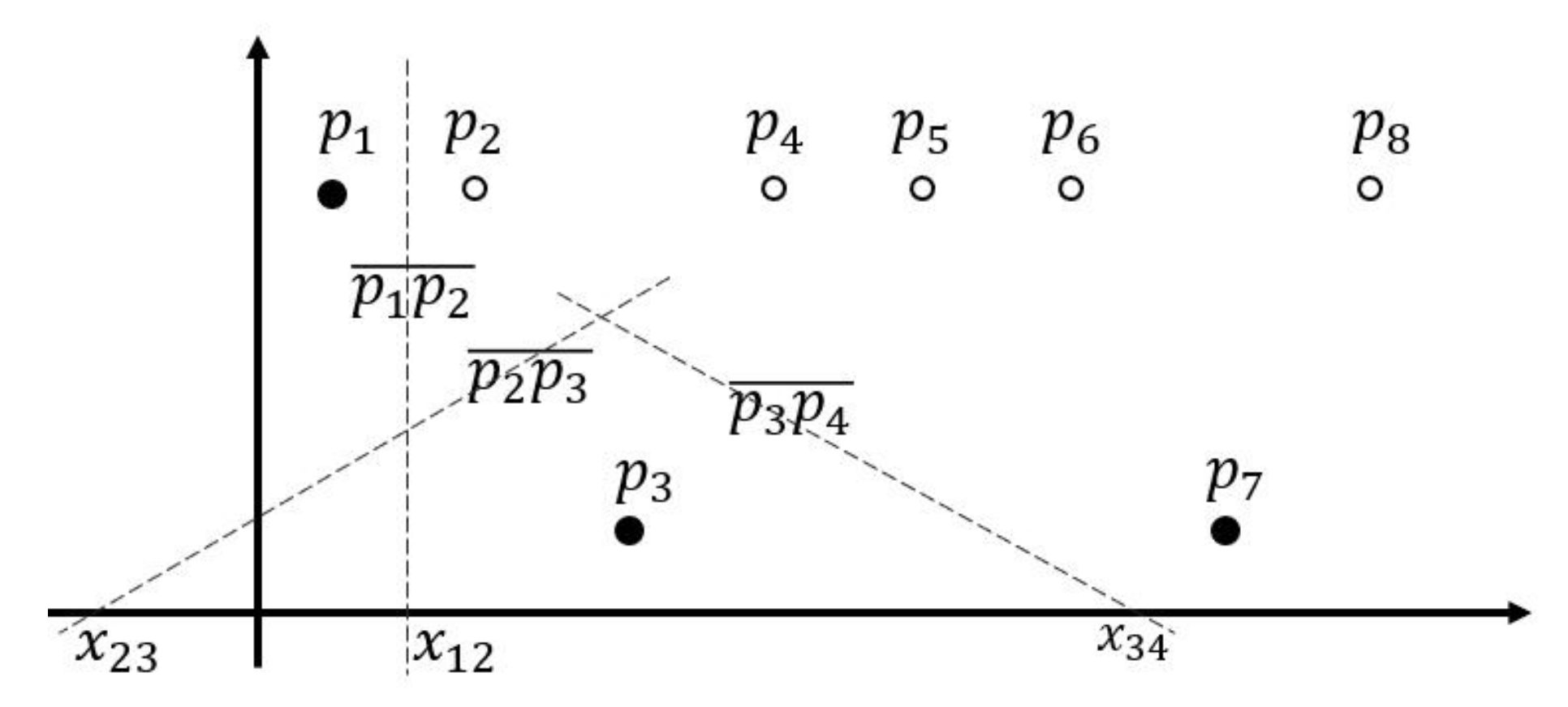
The $key-value$ pairs of step 1 process are sorted and shuffled by column. The Reduce function reads the $key-value$ pairs in the ith column from bottom to up and saves the values into a stack. Notice that every column is saved in its corresponding stack. We project the grids in the same column into a two-dimensional coordinate where x-axis represents the column IDs of grids, which we count them from bottom to up, and the values of y-axis are the results in step 1.2. We name all n points as $p_1,p_2,\dots ,p_n$. Then, we bisect the adjacent two points $p_i=(x_i,y_i)$, and $p_j=(x_j,y_j)$ where ($1\le i<j\le n$). $x_{ij}$ is the intersection of the vertical bisector $\overline{p_i{p}_j}$ and x-axis. We compute $x_{ij}$ by formula (1):

$$\begin{array}{c}\hfill x_{ij}=\frac{(y_j^2-y_i^2)+(x_j^2-x_i^2)}{2(x_j-x_i)}\end{array}$$

(1)

Assume that $p_i,p_j$ and $p_k$ are three adjacent points and ($i<j<k$). We delete $p_j$ from the stack if and only if $x_{ij}>x_{jk}$. Otherwise, we save the point $p_j$ into the stack. Figure 7 and Figure 8 illustrated the two cases whether deleting $p_j$ or not.

Figure 9 demonstrates an example of the step 2.1 process of 5th column of Figure 6. Firstly, we compare $x_{12}$ and $x_{23}$, and delete $p_2$ from the stack. Next, we compare $x_{13}$ and $x_{34}$, and save $p_3$ into the stack. Follow the same procedure until all eight points are encountered. Finally, point $p_1,p_3$ and $p_7$ are saved into the stack. point $p_2,p_4,p_5,p_6$ and $p_8$ are deleted from the stack.

Step 2.2 For the ith column, we compute the distance of the points which are deleted from the stack. Specifically, we bisect the adjacent left points to determine the proximate intervals [21] on x-axis. The interval $[a,b]$ ($a,b\in \mathbb{Z}$ and $a\le b$) of the left point $p_i$ after step 2.1 process determines the dominated areas of point $p_i$.

Figure 10 shows an example of step 2.2 process. $p_1,p_3$ and $p_7$ are the left points of step 2.1. We bisect $p_1,p_3$ and $p_3,p_7$ to calculate $x_{13}<0$ and $x_{37}=5$. The intervals of points $p_3$ and $p_7$ are $[x_{13},x_{37}]$ and $[x_{37},8]$. It means that the point $p_3$ dominates points $p_1,p_2,p_4$ and $p_5$. Points $p_6,p_8$ are dominated by point $p_7$. In the obvious way, we can compute the distance of all grids in the map.

The algorithm of Reduce function is illustrated in Algorithm 2. The input of this step is the $key-value$ pairs. The $key$ is the column ID, and the $value$ is the distance calculated in the Map function. The outputs are the area skyline objects such as the shaded grids shown in Figure 3.

Algorithm 2 Reduce Function for Step 2 Process

Input: The results of the sorted and shuffle phase Output: Area skyline objects 1: for each point sorted by x-coordinate in the same column do 2:     if $x_{ij}>x_{jk}$ then 3:         pop the point $p_j$ from the stack 4:     end if 5: end for 6: for all un-popped points which are sorted by x-coordinate do 7:     calculate the proximate interval of each point on x-axis 8:     calculate the Euclidean Distance of the points in the interval 9: end for 10: //remove the dominated grids 11: for the record $r_i$ of the Euclidean Distance for all types of each grid do 12:     if $r_i<r_j$ then 13:         remove the dominated grid from the record 14:     end if 15: end for 16: return skyline objects

We demonstrate the complete results of the step 2 process of type $F{1}^{+}$ in Figure 11. Note that for the facility type, $F{2}^{+}$ and $F{3}^{-}$ can be calculated in the same process in the MapReduce framework. Intuitively, our proposed MRGASKY algorithm can implement the same process of Voronoi Diagram. However, MRGASKY is a distributed algorithm in MapReduce framework whose complexity is much smaller than the Voronoi Diagram method.

Figure 12 demonstrates MapReduce data flow of facility type $F{1}^{+}$ and $F{2}^{+}$. The input data are stored in HDFS. Specifically, they are formed as facility types F, row IDs n and the values of the binary image in the same row. Next, we separate the data by row-wise and send them to the Map function. In the Map function, the data are processed by $key-value$ pairs. The output of the Map function generates new $key-value$ pairs, and the intermediate $key-value$ pairs are grouped and sorted with the same intermediate keys. After sorted and shuffle phase, the grids in the same column are grouped. Similarity, the grouped data are sent to the Reduce function. The Reduce function mainly calculates the distance of every grid to the nearest facility of each type column-wise.

4. Experimental Evaluation

In this Section, we conduct extensive experiments to evaluate the efficiency and effectiveness of the proposed algorithm. We implement all algorithms using python 3.5.2. We select our previous work GASKY as the baseline and compare it with the proposed MRGASKY algorithm. We conduct GASKY on Linux operating system with Intel Core i7 3.40 GHz processor. It has 4 GB main memory. For the experiments of MRGASKY, there are a total of four compute nodes for the MapReduce framework. One computing node is the PC of GASKY. The remaining three PCs are conducted on Linux operating systems with Intel Core 2 3.16 GHz, 3.16 GHz, and 2.13 GHz processors. These PCs have 4 GB main memories. We implement the MRGASKY algorithm on Hadoop 2.5.2 version.

Synthetic datasets: 

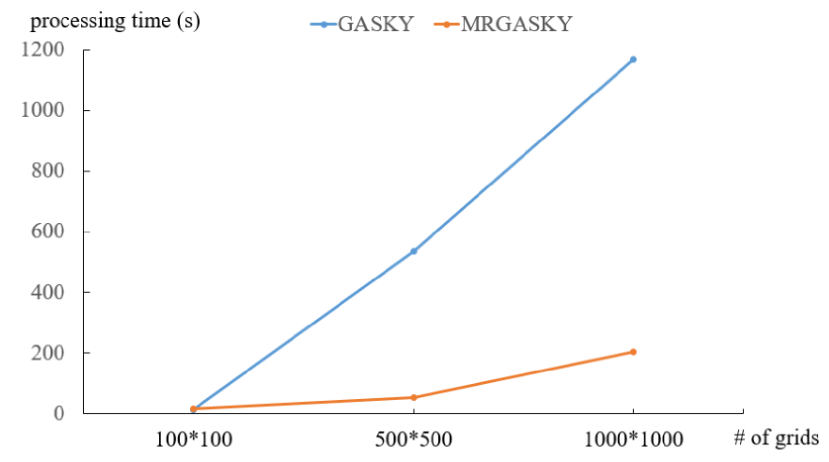
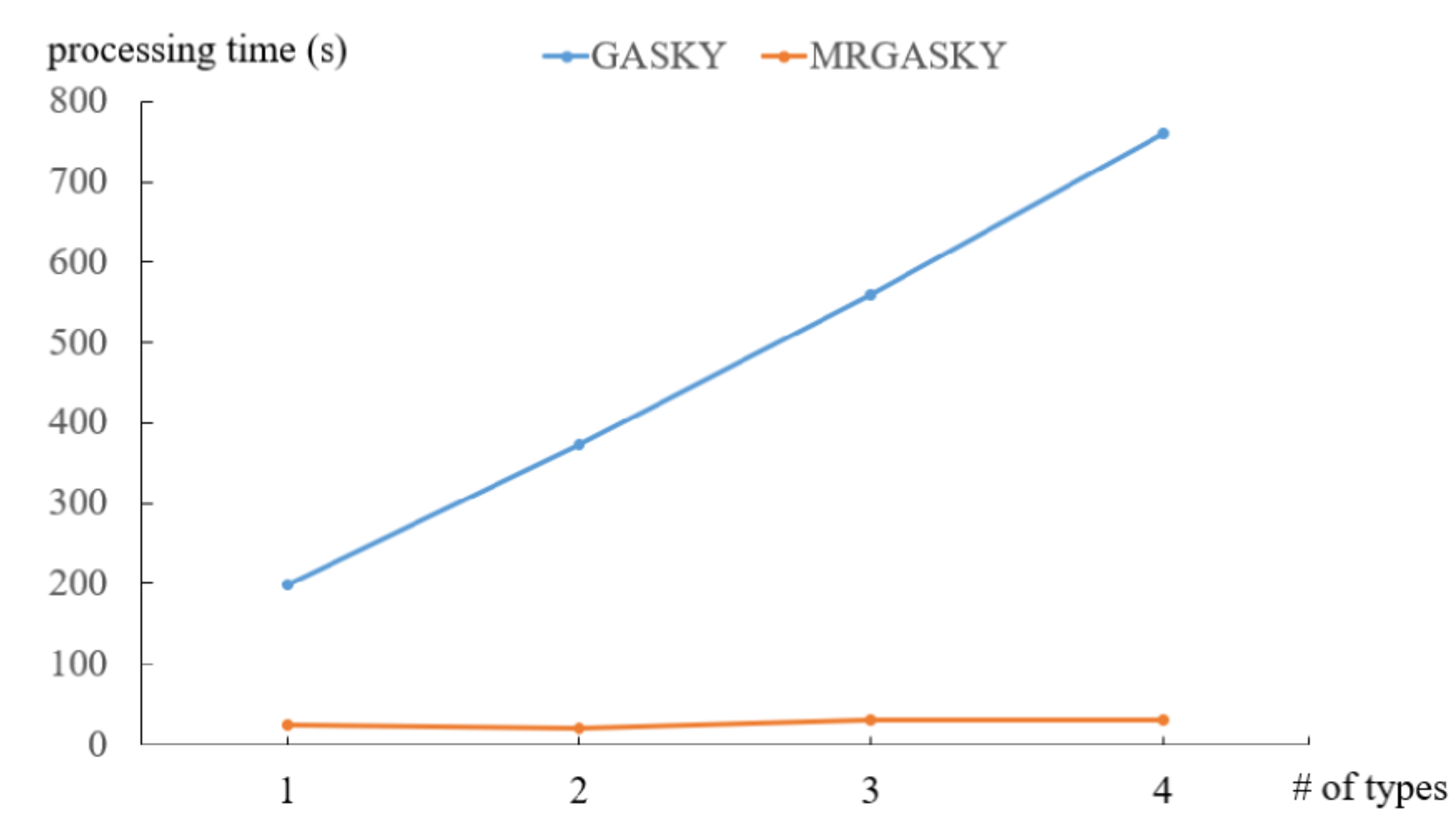
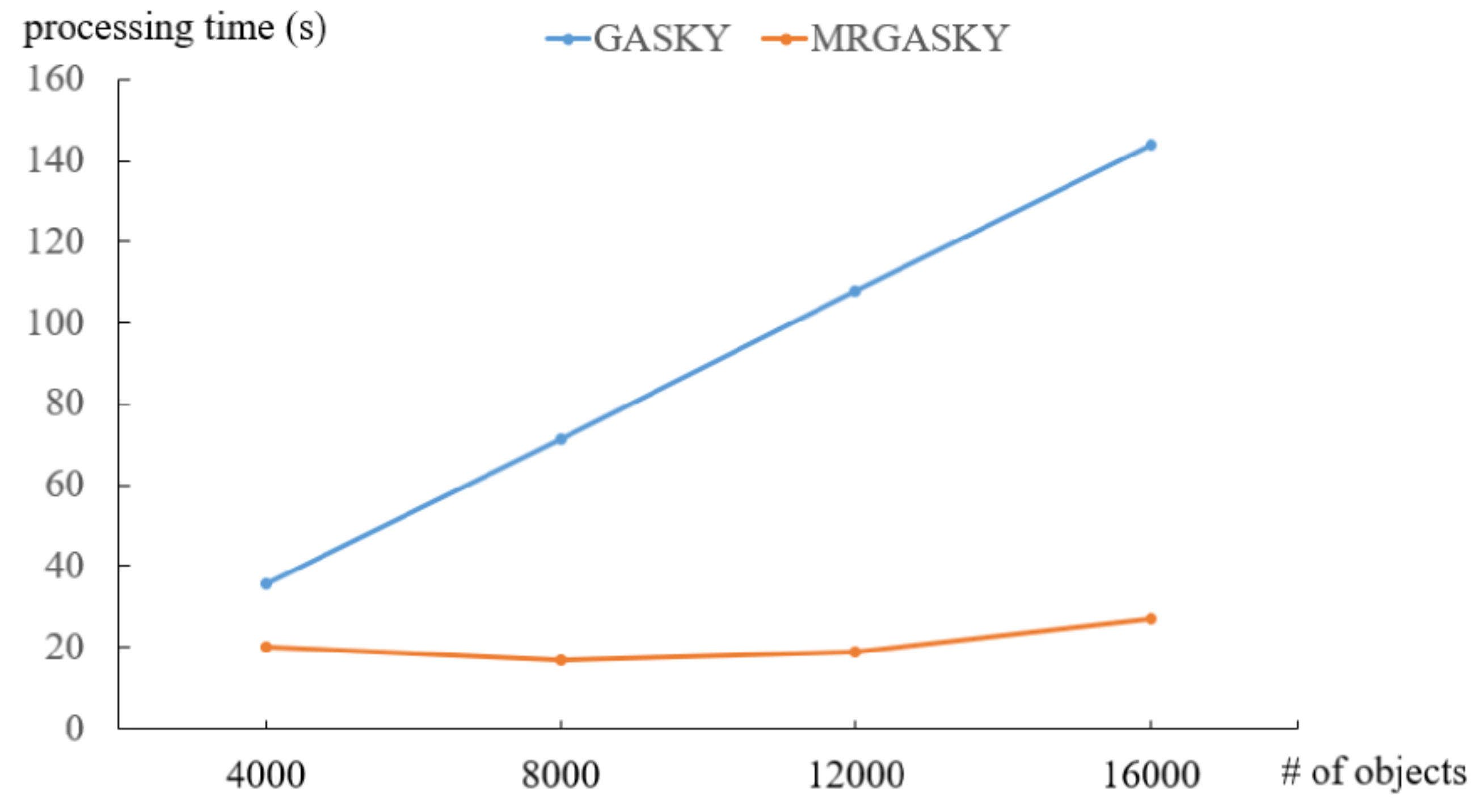
We create a synthetic dataset to study the scalability of the algorithms, denoted by SYN, in the experiments. The objects and facilities are randomly generated in two-dimensional space. Specifically, there are four synthetic datasets, SYN_A1, SYN_A2, SYN_B and SYN_C with different number of grids, number of facility types and number of objects respectively.

Real datasets: 

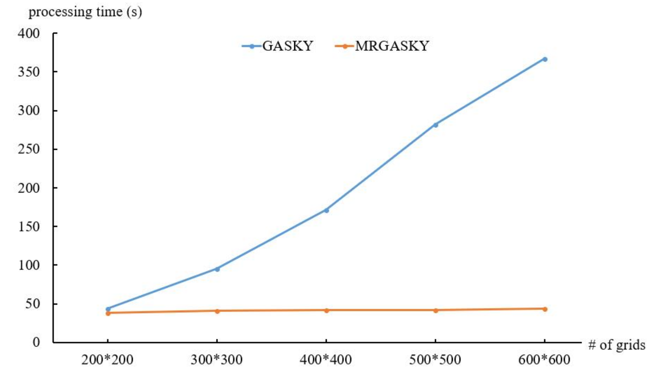
The real dataset, called US, is employed in the experiment. US dataset comes from the U.S. Geological Survey (USGS). It consists of 406,709 locations with 40 types. The number of objects in the US dataset is 2,033,545. We create three datasets by using these real data, denoted US_A, US_B, and US_C, with the different number of grids, facility types and objects respectively.

To compare the performance across the GASKY and the MRGASKY, we evaluate the average processing time. Since it is the same process to remove the dominated objects from the dataset for both two algorithms, and there is no difference in performance evaluation, we do not calculate the time cost of this step.

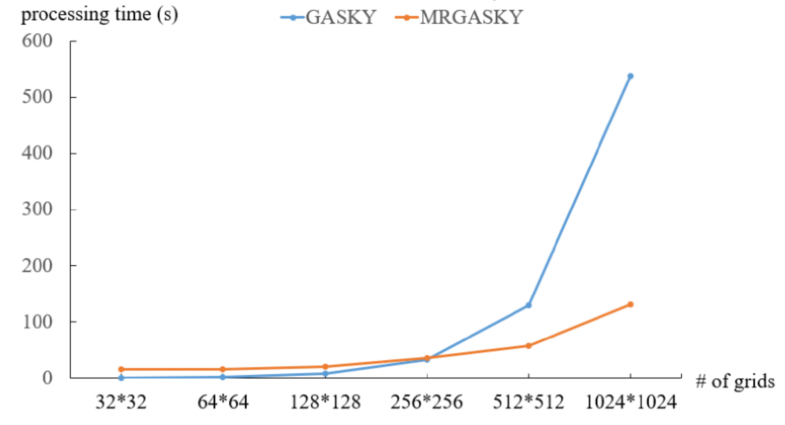
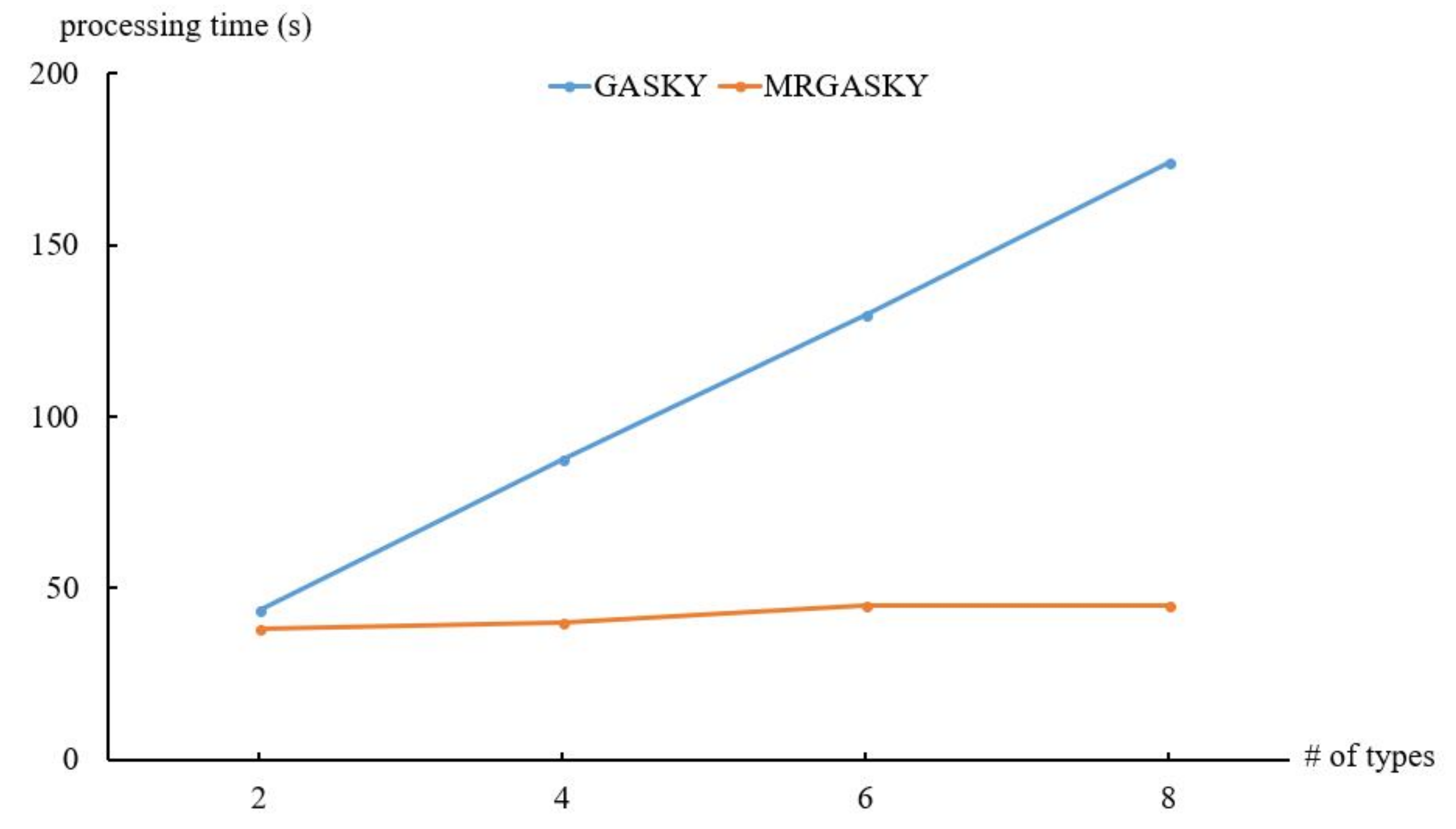
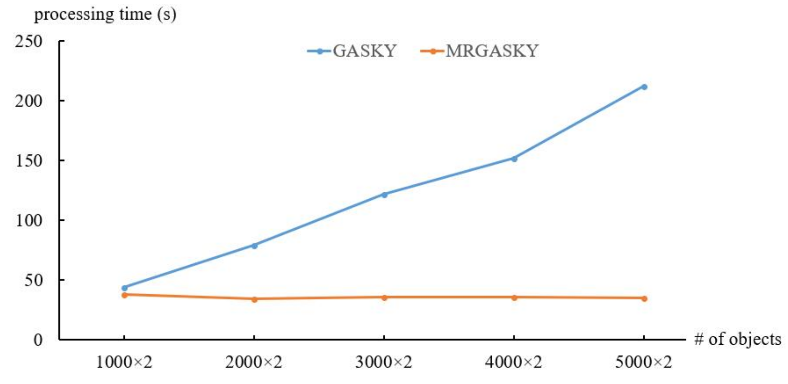
4.1. Efficiency of Synthetic Dataset

In this subsection, we investigate the efficiency of the synthetic dataset.

Effect of grids: For SYN_A1 dataset, we set facility type $m=4$. Both of the number of preferable facility types and unpreferable facility types are two. We vary the number of grids $n^2$ with $32\times 32$, $64\times 64$, $128\times 128$, $512\times 512$ and $1024\times 1024$ respectively. For dataset SYN_A2, a larger dataset than SYN_A1, we fix the number of facility type $m=2$, which consists of one preferable facility type and one unpreferable facility type. The number of objects is set to $obj=2000$. The number of grids are varying as $100\times 100$, $500\times 500$ and $1000\times 1000$.

Figure 13 and Figure 14 show the results. From the results in Figure 13, we find that the processing time increases with the number of grids increasing. Furthermore, the processing time of GASKY algorithm increases faster than MRGASKY algorithm when $n^2$ is larger than $256\times 256$. The results in Figure 14 show that processing time of GASKY algorithm increases faster at the beginning while MRGASKY has a relatively steady increase. In other words, GASKY algorithm takes more time in $min-max$ computation [5] and Voronoi Diagram building. Thus, MRGASKY has better scalability with the increase of the number of grids.

Effect of facility types: In SYN_B, we conduct the effect on the number of facility types. We set the number of objects as $obj=\mathrm{10,000}$ and the number of grids as $128\times 128$. m is varied with 2, 4, 6 and 8 respectively. Both the number of preferable facility types and unpreferable facility types are set to be the same values.

Figure 15 demonstrates the results. We can observe that the average processing time of GASKY algorithm increases linearly when m changes. Conversely, the average processing time of the MRGASKY algorithm is smaller than GASKY and tends to be stable. The result shows that the proposed algorithm outperforms the GASKY, which justifies that our algorithm has good scalability on the facility types.

Effect of objects: In SYN_C, we set $m=2$, $n^2=128\times 128$. The number of objects is varied with 4000, 8000, 12,000 and 16,000.

The result shows in Figure 16. The performance of the MRGASKY algorithm is much better than the GASKY algorithm. Overall, the MRGASKY algorithm maintains sufficient stability to handle “big data”.

4.2. Efficiency of Real Dataset

In this subsection, we conduct the effect of processing time under the different number of grids, facility types, and objects in the real dataset.

Effect of grids: For US_A dataset, we set facility types $m=2$. Both the preferable facility types and unpreferable facility types are 1. We vary the number of grids $n^2$ with $200\times 200$, $300\times 300$, $400\times 400$, $500\times 500$ and $600\times 600$ respectively.

Figure 17 shows the results. We observe that the processing time of our MRGASKY algorithm is particularly stable. In contrast, for GASKY algorithm, the processing time increases very fast with the increase of the number of grids.

Effect of facility types: In US_B, we fix the number of objects $obj=1000$ for each facility type and the number of grids $200\times 200$. We set the number of types m as 2, 4, 6 and 8, respectively.

In Figure 18, we can observe that the number of facility types has a significant effect on the processing time. Moreover, similar to previous experiments, the processing time of our MRGASKY smoothly changes below 50 while GASKY increases from 50.

Effect of objects: In US_C, we vary the number of objects with 2000, 4000, 6000, 8000 and 10,000. The number of grids and the number of facility types are fixed to $m=2$ and $n^2=200\times 200$.

The results are demonstrated in Figure 19. We observe that when the number of objects increases, the processing time also increases. Besides, for the MRGASKY algorithm, the processing time is much smaller than GASKY algorithm.

5. Conclusions

Location recommendation is essential for many map-based mobile applications. In general, a good location should be surrounded by preferable facilities and away from unpreferable facilities. In our previous work, we proposed a grid-based area skyline algorithm, GASKY, to recommend such locations. In this paper, we proposed a novel distributed algorithm, MRGASKY, to improve the performance of area skyline in the MapReduce framework. The experiments are conducted to demonstrate the effectiveness and efficiency of our proposed algorithm. With the number of grids, the number of facility types and the number of objects increases, the processing time of MRGASKY algorithm increases smoothly and slowly. It is confirmed to handle the “big data” effectively.

In addition, some other specific scenarios can also utilize this approach:

• In the business field: Suppose a real estate developer would like to find a region to build a community. In general, a good region of the community should be close to some highly popular places such as bus/train stations, malls, and schools. Besides, it should be far from some unpopular places such as noisy factories and open landfills. Our proposed algorithm can help the real estate developer find some potential areas on a map, which could reduce the survey cost the whole regions.
• In the travel field: It is very common for tourists to utilize map applications on mobile devices during a trip. In most instances, tourists would like to find some sightseeing spots where should be surrounded by preferable facilities and away from unpreferable facilities. Our algorithm can recommend such locations to the users of mobile devices in a short time.

In the future, we would like to consider the $k$-dominant problem and the non-spatial properties such as price, population density, etc., in the MRGASKY algorithm. In addition, we also would like to apply our algorithm in the map applications to help more people to make location recommendations.

References

- Borzsonyi, S.; Kossmann, D.; Stocker, K. The skyline operator. In Proceedings of the 17th International Conference on Data Engineering (ICDE), Heidelberg, Germany, 2–6 April 2001; pp. 421–430. [Google Scholar]
- Chomicki, J.; Godfrey, P.; Gryz, J.; Liang, D. Skyline with presorting. In Proceedings of the 19th International Conference on Data Engineering (ICDE), Bangalore, India, 5–8 March 2003; pp. 717–719. [Google Scholar]
- Tan, K.L.; Eng, P.K.; Ooi, B.C. Efficient progressive skyline computation. In Proceedings of the 27th International Conference on Very Large Data Bases (VLDB), Rome, Italy, 11–14 September 2001; pp. 301–310. [Google Scholar]
- Xia, T.; Zhang, D.; Tao, Y. On skylining with flexible dominance relation. In Proceedings of the 24th International Conference on Data Engineering (ICDE), Cancun, Mexico, 7–12 April 2008; pp. 1397–1399. [Google Scholar]
- Zaman, A.; Morimoto, Y. Area skyline query for selecting good locations in a map. J. Inf. Process 2016, 24, 946–955. [Google Scholar]
- Chan, C.Y.; Jagadish, H.; Tan, K.L.; Tung, A.K.; Zhang, Z. On high dimensional skylines. In Proceedings of the 10 International Conference on Extending Database Technology, Munich, Germany, 26–31 March 2006; pp. 478–495. [Google Scholar]
- Chan, C.Y.; Jagadish, H.; Tan, K.L.; Tung, A.K.; Zhang, Z. Finding k-dominant skylines in high dimensional space. In Proceedings of the International Conference on Management of Data and Symposium on Principles Database and Systems, Chicago, IL, USA, 27–29 June 2006; pp. 444–457. [Google Scholar]
- Lin, X.; Yuan, Y.; Zhang, Q.; Zhang, Y. Selecting stars: The k most representative skyline operator. In Proceedings of the 23rd International Conference on Data Engineering, Istanbul, Turkey, 11–15 April 2007; pp. 86–95. [Google Scholar]
- Sharifzadeh, M.; Shahabi, C. The Spatial Skyline Queries. In Proceedings of the 32nd International Conference on Very Large Data Bases (VLDB), Seoul, Korea, 12–15 September 2006; pp. 751–762. [Google Scholar]
- Kodama, K.; Iijima, Y.; Guo, X.; Ishikawa, Y. Skyline queries based on user locations and perferences for making location-based recommendations. In Proceedings of the 19th International Workshop on Location Based Social Networks (LBSN), Washington, DC, USA, 3 November 2009; pp. 9–16. [Google Scholar]
- Arefin, M.; Xu, J.; Chen, Z.; Morimoto, Y. Skyline query for selecting spatial objects by utilizing surrounding objects. J. Softw. 2013, 8, 1742–1749. [Google Scholar] [CrossRef]
- You, G.W.; Lee, M.W.; Im, H.; Hwang, S.W. The farthest spatial skyline queries. Inf. Syst. 2013, 38, 286–301. [Google Scholar] [CrossRef]
- Lin, Y.W.; Wang, E.T.; Chiang, C.F.; Chen, A.L.P. Finding targets with the nearst favor neighbor and farthest disfavor neighbor by a skyline query. In Proceedings of the 29th Annual ACM Symposium on Applied Computing (SAC), Gyeongju, Korea, 24–28 March 2014; pp. 821–826. [Google Scholar]
- Siddique, M.A.; Zaman, A.; Morimoto, Y. A Method for selecting desirable unfixed shape areas from integrated geographic information system. In Proceedings of the 4th International Congress on Advanced Applied Informatics, Okayama, Japan, 12–16 July 2015; pp. 195–200. [Google Scholar]
- Hose, K.; Vlachou, A. A survey of skyline processing in highly distributed environments. Int. J. Very Large Data Bases 2012, 21, 359–354. [Google Scholar] [CrossRef]
- Zhang, B.; Zhou, S.; Guan, J. Adapting skyline computation to the mapreduce framework: Algorithms and experiments. In Proceedings of the 16th International Conference on Database Systems for Advanced Applications, Hong Kong, China, 22–25 April 2011; pp. 403–414. [Google Scholar]
- Chen, L.; Hwang, K.; Wu, J. MapReduce skyline query processing with new angular partitioning approach. In Proceedings of the 2012 IEEE 26th International Parallel and Distributed Processing Symposium Workshops and PhD Forum, Shanghai, China, 21–25 May 2012; pp. 2262–2270. [Google Scholar]
- Papadias, D.; Tao, Y.; Fu, G.; Seeger, B. Progressive skyline computation in database systems. ACM Trans. Database Syst. 2005, 30, 41–82. [Google Scholar] [CrossRef]
- Wu, P.; Zhang, C.; Feng, Y.; Zhao, B.; Agrawal, D.; Abbadi, A. Parallelizing skyline queries for scalable distribution. In Proceedings of the 10 International Conference on Extending Database Technology, Munich, Germany, 26–31 March 2006. [Google Scholar]
- Wang, W.; Zhang, J.; Sun, M.T.; Ku, W.S. Efficient parallel spatial skyline evaluation using MapReduce. In Proceedings of the 20th International Conference on Extending Database Technology, Venice, Italy, 21–24 March 2017. [Google Scholar]
- Man, D.; Uda, K.; Ito, Y.; Nakano, K. Accelerating computation of Euclidean distance map using the GPU with efficient memory access. Int. J. Parallel Emergent Distrib. Syst. 2012, 25, 383–406. [Google Scholar] [CrossRef]