Best Trade-Off Point Method for Efficient Resource Provisioning in Spark


Abstract
:1. Introduction
2. Best Trade-Off Point (BToP) Method
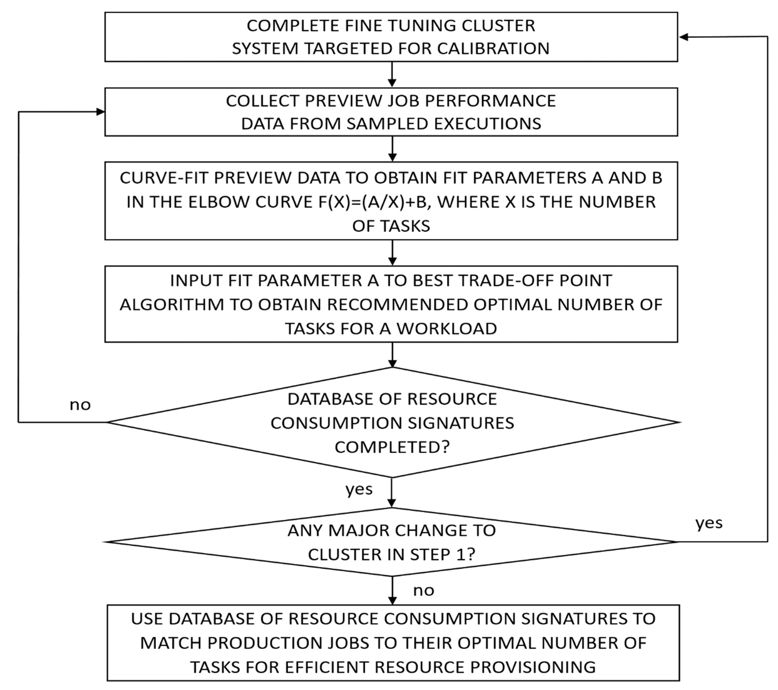
- Step 1.
- Complete the configuration and fine tuning of the architecture, software, and hardware of the production cluster-computing system targeted for calibration.
- Step 2.
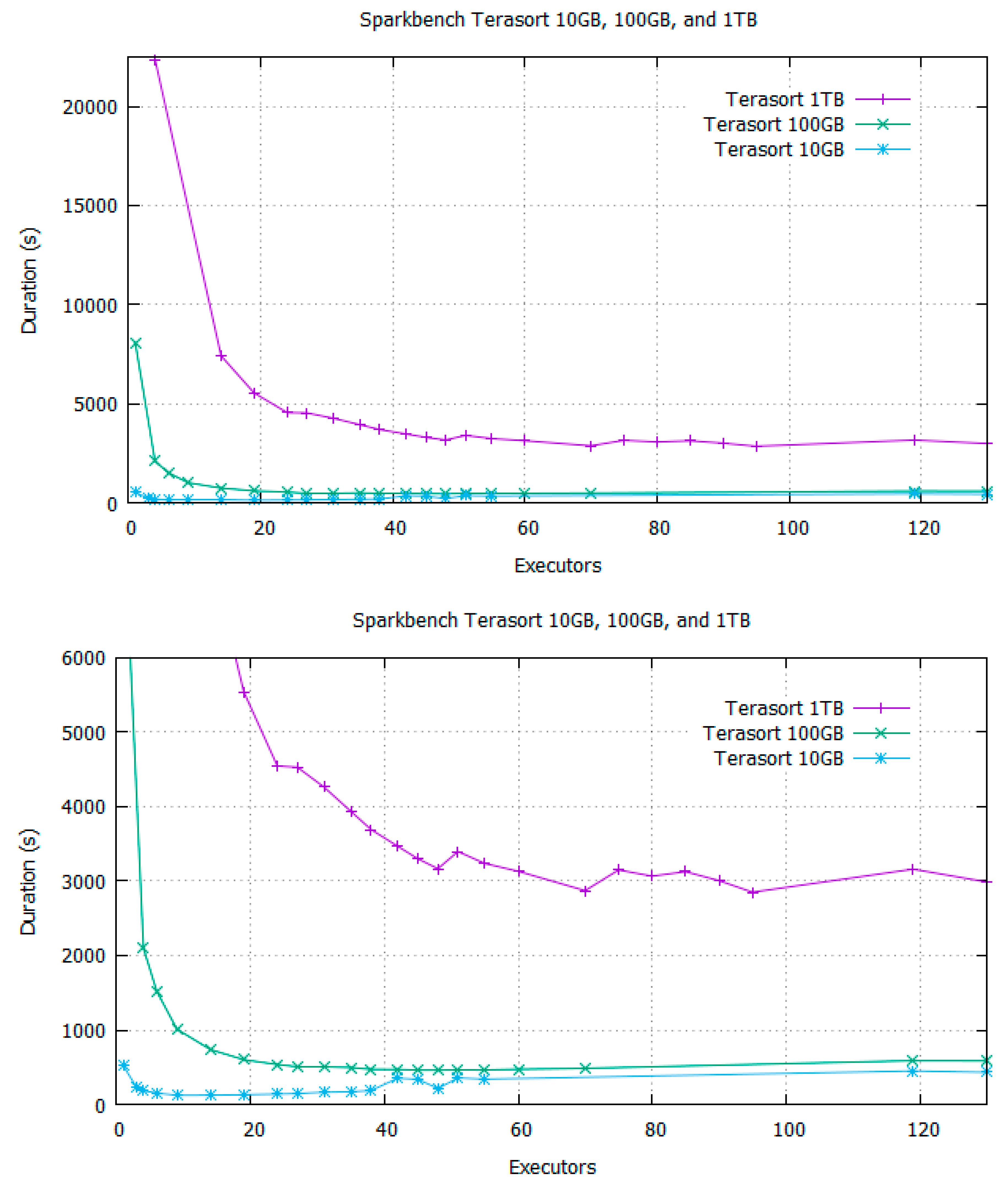
- Collect necessary preview job performance data from historical runtime performances or sampled executions on the same target production system, configured exactly as in step 1, as reference points for each workload.
- Step 3.
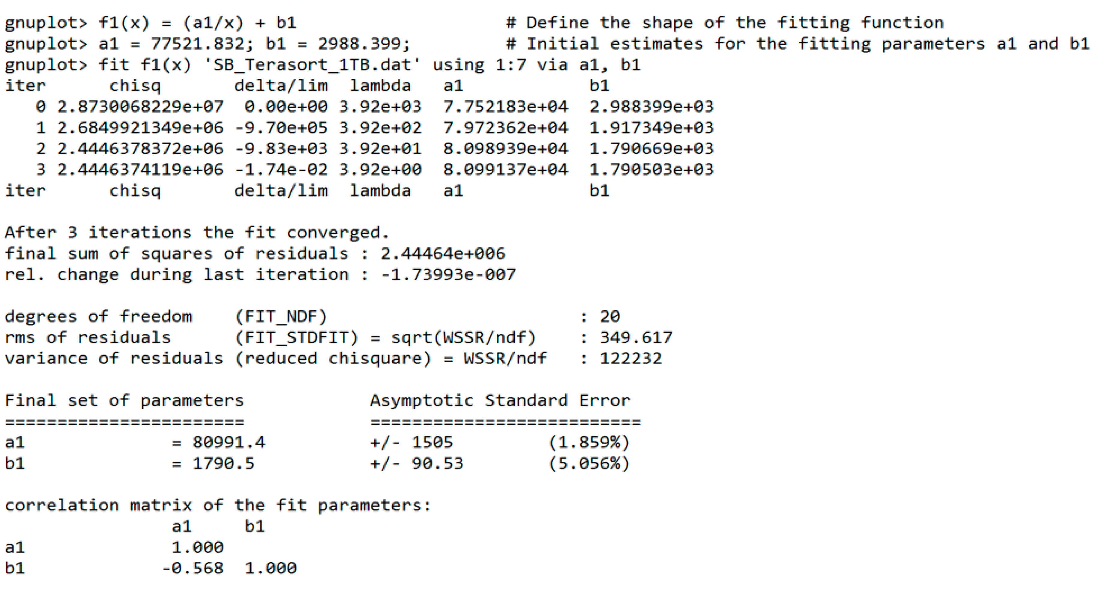
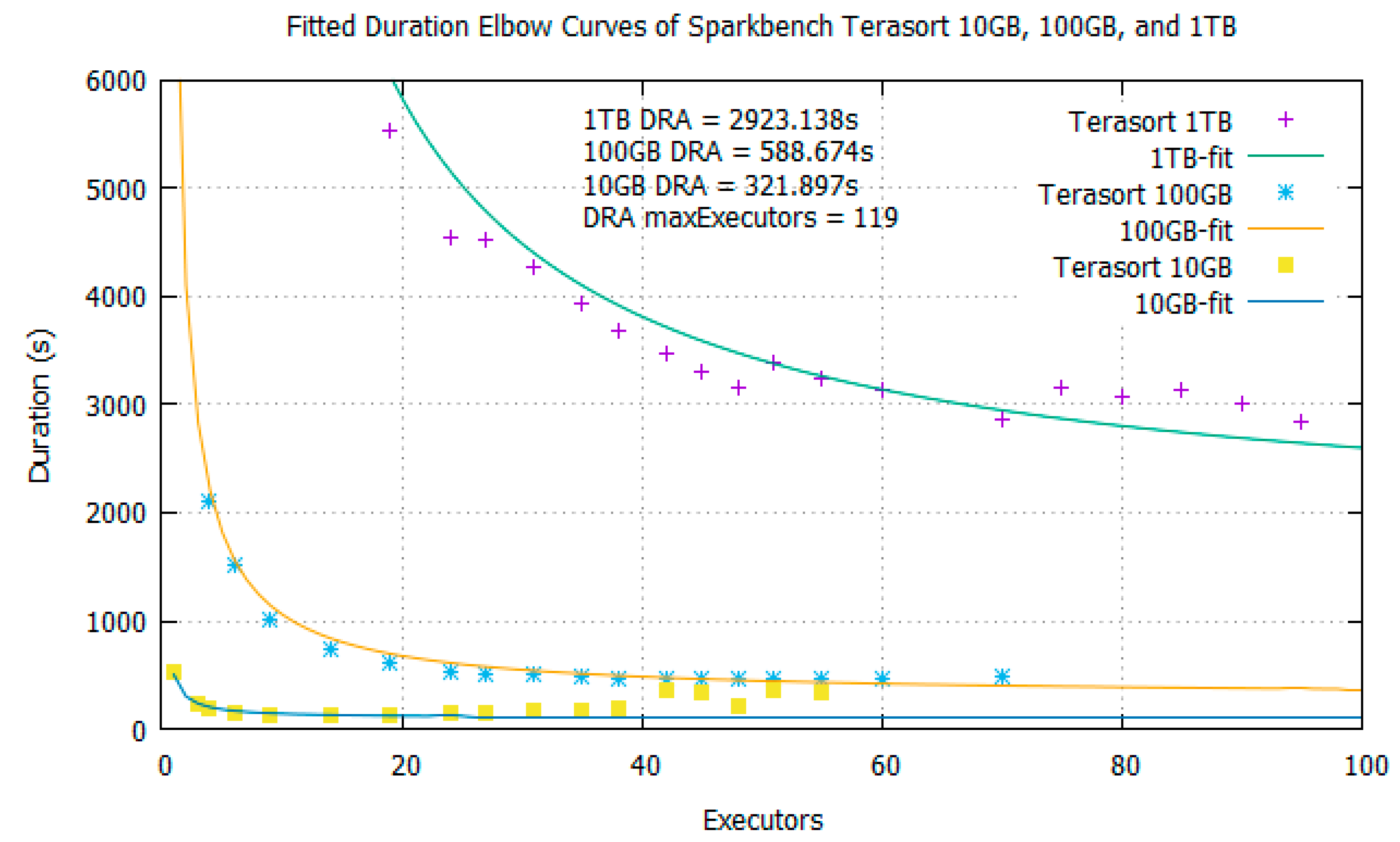
- Curve-fit the preview data to obtain the fit parameters a and b in the runtime elbow curve function f(x) = (a/x) + b, where x is the number of executor resources.
- Step 4.
- Input the fit parameter a to the BToP algorithm to obtain the recommended optimal number of executors for a workload (Algorithms 1 and 2).
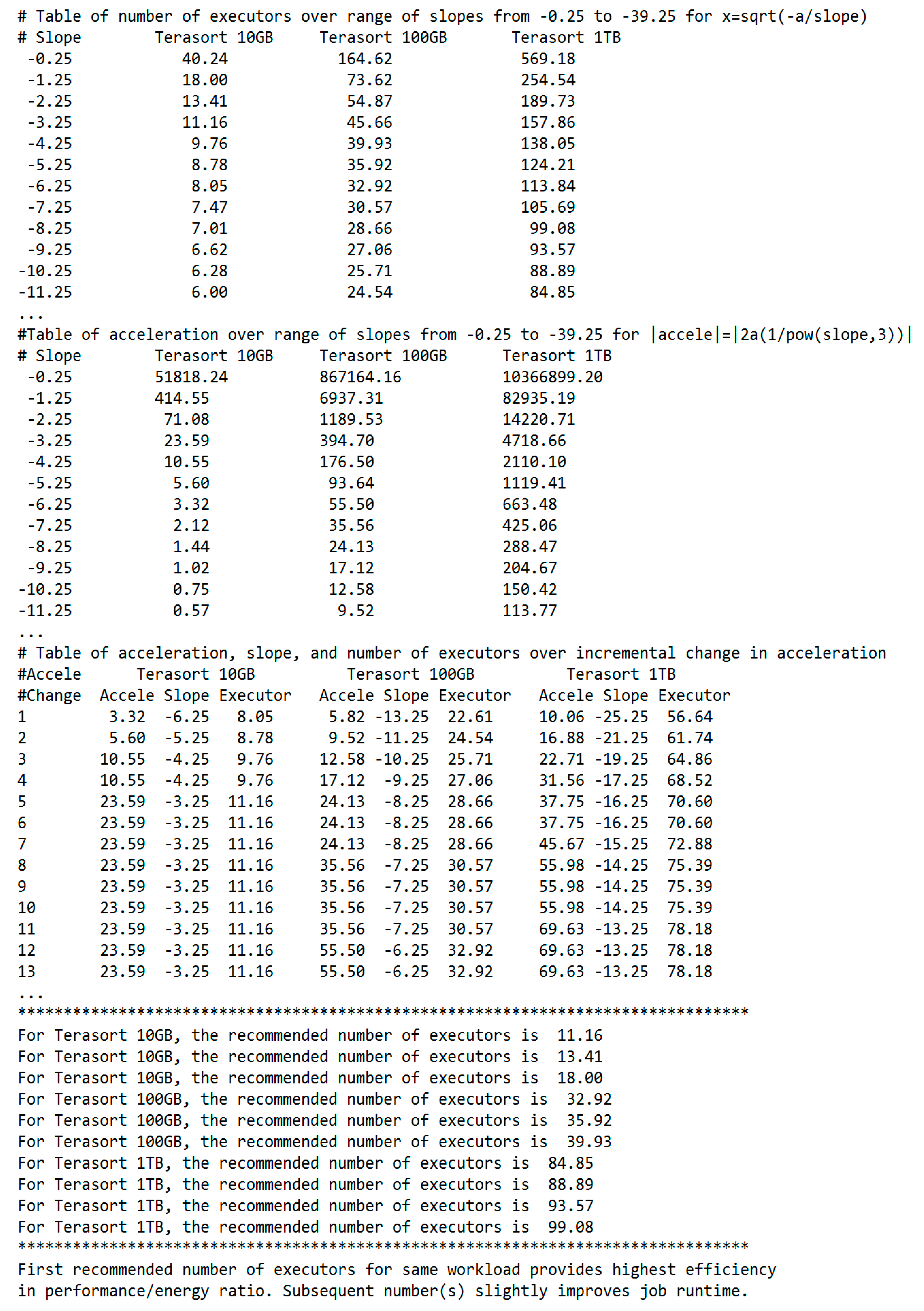
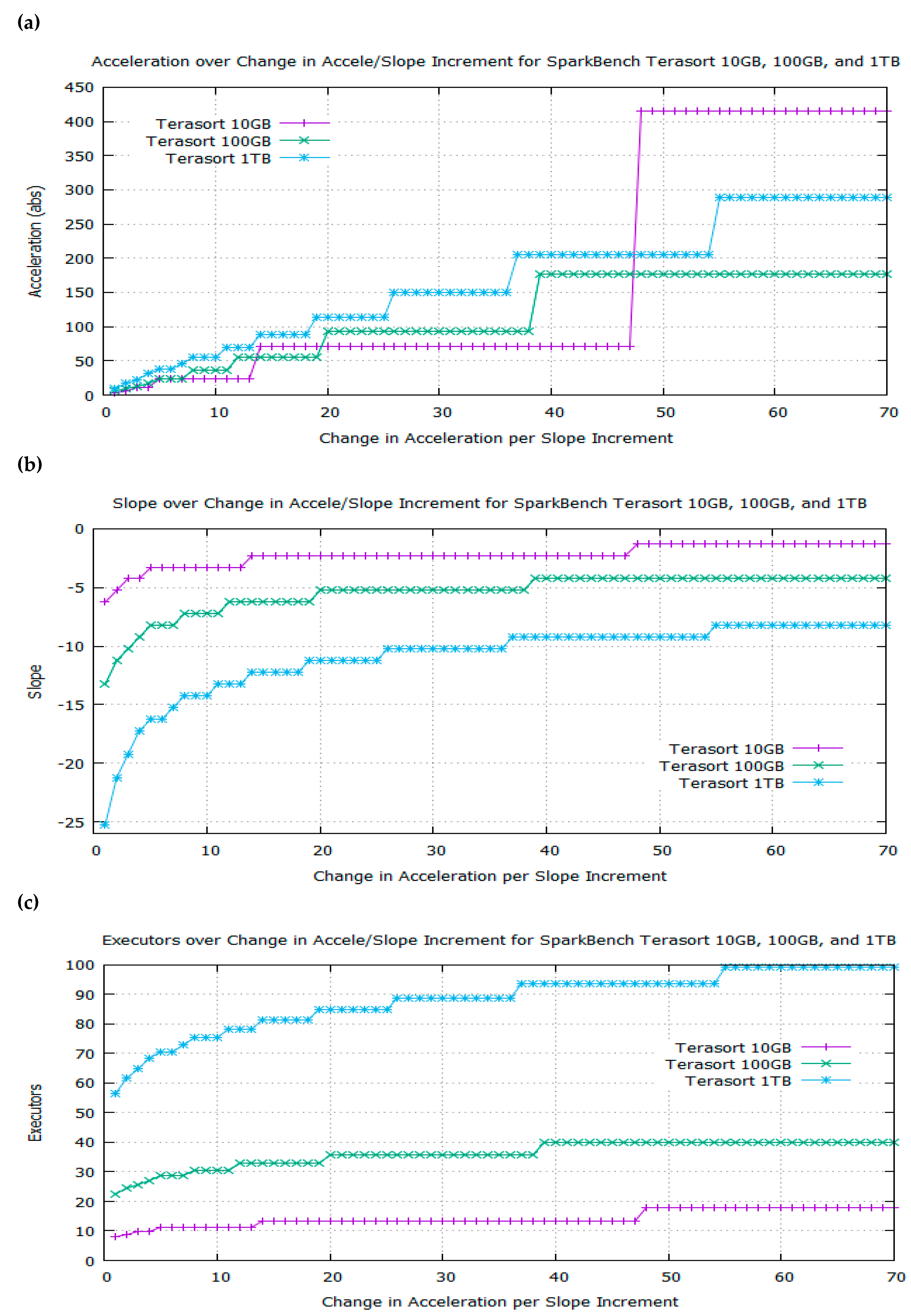
- The algorithm computes the number of executors over a range of slopes from the first derivative of f(x) = (a/x) + b and the acceleration over a range of slopes from the second derivative (Algorithms 1 and 2).
- The algorithm applies the Chain Rule to search for break points and major plateaus on the graphs of acceleration, slope, and executor resources over a range of incremental changes in acceleration per slope increment (Algorithms 1 and 2).
- The algorithm extracts the exact number of executors at the best trade-off point on the elbow curve and outputs it as the recommended optimal number of executors for a workload (Algorithms 1 and 2).
- Step 5.
- Repeat steps 2–4 to gather enough resource provisioning data points for different workloads to build a database of resource consumption signatures for subsequent job profiling.
- Step 6.
- Repeat steps 1–5 to recalibrate the database of resource consumption signatures if there are any major changes to step 1.
- Step 7.
- Use the database of resource consumption signatures to match dynamically submitted production jobs to their recommended optimal number of executors for efficient resource provisioning.
| Algorithm 1: Best Trade-off Point for a non-inverted elbow curve f(x) = (a/x) + b |
| Input: Parameter a for a workload with runtime curve f(x) = (a/x) + b |
| Output: Optimal number of executors |
| foreach incremental slope value do |
| output number of executors x=sqrt(-a/slope); |
| end |
| foreach incremental slope value do |
| output absolute value of acceleration=2a/pow(slope, 3); |
| end |
| foreach incremental target value of change in acceleration do |
| foreach incremental slope value do |
| if change in acceleration in the current slope increment is >= to the target value AND change in acceleration in the next slope increment is < the target value then output acceleration, slope, and number of executors; store number of tasks in an array register; break; |
| end |
| end |
| end |
| foreach incremental target of change in acceleration do |
| if number of executors do not change in 7 increments then |
| output number of executors as recommended optimal value; break; |
| end |
| end |
| Algorithm 2: Best Trade-off Point for an inverted elbow curve f(x) = −(a/x) + b |
| Input: Parameter a for a workload with runtime curve f(x) = −(a/x) + b |
| output: Optimal number of executors |
| foreach incremental slope value do |
| output number of executors x=sqrt(a/slope); |
| end |
| foreach incremental slope value do |
| output absolute value of acceleration=-2a/pow(slope, 3); |
| end |
| foreach incremental target value of change in acceleration do |
| foreach incremental slope value do |
| if change in acceleration in the current slope increment is >= to the target value AND change in acceleration in the next slope increment is < the target value then output acceleration, slope, and number of executors; store number of tasks in an array register; break; |
| end |
| end |
| end |
| foreach incremental target of change in acceleration do |
| if number of executors do not change in 7 increments then output number of executors as recommended optimal value; break; |
| end |
| end |
3. Resource Provisioning in Apache Spark
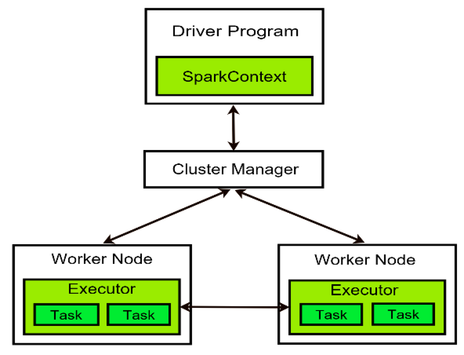
3.1. Spark Architecture and Resilient Distributed Dataset (RDD)
3.2. Distributed Execution in Spark
3.3. Spark’s Dynamic Resource Allocation (DRA)
4. Spark-Bench Terasort Experiment with BToP Method
4.1. Test System Specifications
4.2. Spark Configuration in the Experiment
4.3. BToP Method Implementation in Spark
5. Analysis of Spark with BToP method vs. Spark with DRA Enabled
5.1. Performance Gain
5.2. Energy Saving
= 10,979,37.1 j = 3049.95 Wh per job
= 8,569,808.4 j = 2380.5 Wh per job
6. Related Work
6.1. Performance Prediction Models
6.2. Optimal Resource Ratio by Distribution Probability
6.3. Resource Scheduling Algorithm
6.4. Energy Conservation Algorithm
7. Conclusions
8. Patents
Funding
Acknowledgments
Conflicts of Interest
References
- Gartner’s Forecast of 25 Billion IoT Devices Connected by 2020. Available online: http://www.gartner.com/newsroom/id/2905717 (accessed on 29 August 2018).
- Koomey, J. Growth in data center electricity use 2005 to 2010. A Report by Analytical Press, Completed at the Request of The New York Times. 2011, 9. Available online: https://www.missioncriticalmagazine.com/ext/resources/MC/Home/Files/PDFs/Koomey_Data_Center.pdf (accessed on 29 August 2018).
- Datacenter Knowledge. Available online: http://www.datacenterknowledge.com/archives/2017/03/16/google-data-center-faq (accessed on 29 August 2018).
- Whitney, J.; Delforge, P. Data center efficiency assessment. Nat. Resour. Def. Counc. 2014. Available online: https://www.nrdc.org/sites/default/files/data-center-efficiency-assessment-IP.pdf (accessed on 29 August 2018).
- Nghiem, P.P.; Figueira, S.M. Towards efficient resource provisioning in MapReduce. J. Parallel Distrib. Comput. 2016, 95, 29–41. [Google Scholar] [CrossRef]
- Taran, V.; Alienin, O.; Stirenko, S.; Gordienko, Y.; Rojbi, A. Performance evaluation of distributed computing environments with Hadoop and Spark frameworks. In Proceedings of the 2017 IEEE International Young Scientists Forum on Applied Physics and Engineering (YSF), Lviv, Ukraine, 17–20 October 2017; pp. 80–83. [Google Scholar] [CrossRef]
- Samadi, Y.; Zbakh, M.; Tadonki, C. Performance comparison between Hadoop and Spark frameworks using HiBench benchmarks. Concurr. Comput. Pract. Exp. 2018, 30, e4367. [Google Scholar] [CrossRef]
- Shi, J.; Qiu, Y.; Minhas, U.F.; Jiao, L.; Wang, C.; Reinwald, B.; Özcan, F. Clash of the titans: Mapreduce vs. spark for large scale data analytics. Proc. VLDB Endow. ACM 2015, 8, 2110–2121. [Google Scholar] [CrossRef]
- Kang, M.; Lee, J.G. An experimental analysis of limitations of MapReduce for iterative algorithms on Spark. Clust. Comput. 2017, 20, 3593–3604. [Google Scholar] [CrossRef]
- Kang, M.; Lee, J.G. A comparative analysis of iterative MapReduce systems. In Proceedings of the Sixth International Conference on Emerging Databases: Technologies, Applications, and Theory, ACM, Jeju Island, Korea, 17–19 October 2016; pp. 61–64. [Google Scholar] [CrossRef]
- Veiga, J.; Expósito, R.R.; Taboada, G.L.; Tourino, J. Enhancing in-memory efficiency for MapReduce-based data processing. J. Parallel Distrib. Comput. 2018. [Google Scholar] [CrossRef]
- Databricks. Available online: https://databricks.com/spark/about (accessed on 29 August 2018).
- Babu, S. Towards automatic optimization of MapReduce programs. In Proceedings of the 1st ACM symposium on Cloud computing, ACM, Indianapolis, IN, USA, 10–11 June 2010; pp. 137–142. [Google Scholar] [CrossRef]
- Herodotou, H.; Dong, F.; Babu, S. No one (cluster) size fits all: Automatic cluster sizing for data-intensive analytics. In Proceedings of the 2nd ACM Symposium on Cloud Computing, Cascais, Portugal, 26–28 October 2011; p. 18. [Google Scholar] [CrossRef]
- Verma, A.; Cherkasova, L.; Campbell, R.H. Resource provisioning framework for mapreduce jobs with performance goals. In Proceedings of the ACM/IFIP/USENIX International Conference on Distributed Systems Platforms and Open Distributed Processing, Lisbon, Portugal, 12–16 December 2011; Springer: Berlin/Heidelberg, Germany, 2011; pp. 165–186. [Google Scholar] [CrossRef]
- Kambatla, K.; Pathak, A.; Pucha, H. Towards Optimizing Hadoop Provisioning in the Cloud. HotCloud 2009, 9, 12. [Google Scholar]
- Apache Hadoop. Available online: http://hadoop.apache.org (accessed on 29 August 2018).
- Apache Spark. Available online: http://spark.apache.org (accessed on 29 August 2018).
- Apache Spark Dynamic Resource Allocation. Available online: http://spark.apache.org/docs/latest/job-scheduling.html#dynamic-resource-allocation (accessed on 29 August 2018).
- Cloudera. Spark Dynamic Allocation. Available online: http://www.cloudera.com/content/www/en-us/documentation/enterprise/latest/topics/cdh_ig_running_spark_on_yarn.html#concept_zdf_rbw_ft_unique_1 (accessed on 29 August 2018).
- Karau, H.; Konwinski, A.; Wendell, P.; Zaharia, M. Learning Spark: Lightning-Fast Big Data Analysis; O’Reilly Media, Inc.: Sebastopol, CA, USA, 2015; ISBN 9781449359065. [Google Scholar]
- Zaharia, M.; Chowdhury, M.; Das, T.; Dave, A.; Ma, J.; McCauley, M.; Stoica, I. Resilient distributed datasets: A fault-tolerant abstraction for in-memory cluster computing. In Proceedings of the 9th USENIX conference on Networked Systems Design and Implementation, San Jose, CA, USA, 25–27 April 2012; p. 2. [Google Scholar]
- Zaharia, M.; Chowdhury, M.; Franklin, M.J.; Shenker, S.; Stoica, I. Spark: Cluster computing with working sets. HotCloud 2010, 10, 95. [Google Scholar]
- Databricks: Understanding your Apache Spark Application Through Visualization. Available online: https://databricks.com/blog/2015/06/22/understanding-your-spark-application-through-visualization.html (accessed on 29 August 2018).
- Agrawal, D.; Butt, A.; Doshi, K.; Larriba-Pey, J.L.; Li, M.; Reiss, F.R.; Xia, Y. SparkBench—A spark performance testing suite. In Proceedings of the Technology Conference on Performance Evaluation and Benchmarking, Kohala Coast, HI, USA, 31 August 2015; Springer: Cham, Switzerland, 2015; pp. 26–44. [Google Scholar] [CrossRef]
- Li, M.; Tan, J.; Wang, Y.; Zhang, L.; Salapura, V. SparkBench: A spark benchmarking suite characterizing large-scale in-memory data analytics. Clust. Comput. 2017, 20, 2575–2589. [Google Scholar] [CrossRef]
- Li, M.; Tan, J.; Wang, Y.; Zhang, L.; Salapura, V. Sparkbench: A comprehensive benchmarking suite for in memory data analytic platform spark. In Proceedings of the 12th ACM International Conference on Computing Frontiers, Ischia, Italy, 18–21 May 2015; p. 53. [Google Scholar] [CrossRef]
- Sparkbench: Benchmark Suite for Apache Spark. Available online: https://sparktc.github.io/spark-bench/ (accessed on 29 August 2018).
- Ullah, S.; Awan, M.D.; Sikander Hayat Khiyal, M. Big Data in Cloud Computing: A Resource Management Perspective. Sci. Progr. 2018. [Google Scholar] [CrossRef]
- IBM Hadoop Dev/Tech Tip/Spark/Beginner’s Guide: Apache Spark Troubleshooting. Available online: https://developer.ibm.com/hadoop/2016/02/16/beginners-guide-apache-spark-troubleshooting/ (accessed on 29 August 2018).
- Hortonworks. Managing CPU resources in your Hadoop YARN clusters, by Varun Vasudev. Available online: https://hortonworks.com/blog/managing-cpu-resources-in-your-hadoop-yarn-clusters/ (accessed on 29 August 2018).
- DZone/Big Data Zone. Using YARN API to Determine Resources Available for Spark Application Submission: Part II. Available online: https://dzone.com/articles/alpine-data-how-to-use-the-yarn-api-to-determine-r (accessed on 29 August 2018).
- Cloudera. How-to: Tune Your Apache Spark Jobs (Part 2). Available online: http://blog.cloudera.com/blog/2015/03/how-to-tune-your-apache-spark-jobs-part-2/ (accessed on 29 August 2018).
- GNUplot. Available online: http://www.gnuplot.info/ (accessed on 29 August 2018).
- Chen, Y.; Keys, L.; Katz, R.H. Towards energy efficient mapreduce. EECS Department, University of California, Berkeley, Technical Report; UCB/EECS-2009-109, 120; University of California, Berkeley: Berkeley, CA, USA, 2009. [Google Scholar]
- Duan, K.; Fong, S.; Song, W.; Vasilakos, A.V.; Wong, R. Energy-Aware Cluster Reconfiguration Algorithm for the Big Data Analytics Platform Spark. Sustainability 2017, 9, 2357. [Google Scholar] [CrossRef]
- Leverich, J.; Kozyrakis, C. On the energy (in) efficiency of hadoop clusters. ACM SIGOPS Oper. Syst. Rev. 2010, 44, 61–65. [Google Scholar] [CrossRef]
- Rivoire, S.; Ranganathan, P.; Kozyrakis, C. A Comparison of High-Level Full-System Power Models. HotPower 2008, 8, 32–39. [Google Scholar]
- U.S. Energy Information Administration. Electric Power Monthly Data for May 2017. Available online: https://www.eia.gov/electricity/monthly/epm_table_grapher.php?t=epmt_5_06_a (accessed on 29 August 2018).
- Wang, K.; Khan, M.M.H. Performance prediction for apache spark platform. In Proceedings of the 2015 IEEE 17th International Conference on High Performance Computing and Communications (HPCC), 2015 IEEE 7th International Symposium on Cyberspace Safety and Security (CSS), 2015 IEEE 12th International Conference on Embedded Software and Systems (ICESS), New York, NY, USA, 24–26 August 2015; pp. 166–173. [Google Scholar] [CrossRef]
- He, H.; Li, Y.; Lv, Y.; Wang, Y. Exploring the power of resource allocation for Spark executor. In Proceedings of the 2016 7th IEEE International Conference on Software Engineering and Service Science (ICSESS), Beijing, China, 26–28 August 2016; pp. 174–177. [Google Scholar] [CrossRef]
- Xu, G.; Xu, C.Z.; Jiang, S. Prophet: Scheduling executors with time-varying resource demands on data-parallel computation frameworks. In Proceedings of the 2016 IEEE International Conference on Autonomic Computing (ICAC), Wuerzburg, Germany, 17–22 July 2016; pp. 45–54. [Google Scholar] [CrossRef]


| Spark-Bench Terasort | DRA Enabled (s) | BToP Method (DRA Disabled) | Improved Performance (%) | |
|---|---|---|---|---|
| Executors | Duration (s) | |||
| 10 GB | 321.897 s | 11 | 129.43 | 59.79 |
| 13 | 122.06 | 62.08 | ||
| 18 | 114.70 | 64.37 | ||
| 100 GB | 588.674 s | 33 | 513.50 | 12.77 |
| 36 | 498.77 | 15.27 | ||
| 40 | 477.73 | 18.85 | ||
| 1 TB | 2923.138 s | 85 | 2739.04 | 6.30 |
| 89 | 2694.84 | 7.81 | ||
| 94 | 2644.34 | 9.54 | ||
| 99 | 2608.56 | 10.76 | ||
| Spark-Bench | DRA Enabled | BToP Method (DRA Disabled) | Energy Saving | ||||||
|---|---|---|---|---|---|---|---|---|---|
| Terasort | Max Exec. | Equiv. Nodes | Energy (Wh/job) | Static Exec. | Equiv. Nodes | Energy (Wh/job) | Per Job (%) | Per Year (kWh) | Per Year ($) |
| 10 GB | 80 | 10 | 398.36 | 18 | 3 | 188.37 | 52.71 | 2207.41 | 329.57 |
| 100 GB | 120 | 15 | 770.60 | 40 | 5 | 330.53 | 57.11 | 4626.02 | 690.66 |
| 1 TB | 120 | 15 | 3049.95 | 99 | 13 | 2380.5 | 21.95 | 7037.26 | 1050.66 |
© 2018 by the author. Licensee MDPI, Basel, Switzerland. This article is an open access article distributed under the terms and conditions of the Creative Commons Attribution (CC BY) license (http://creativecommons.org/licenses/by/4.0/).
Share and Cite
Nghiem, P.P. Best Trade-Off Point Method for Efficient Resource Provisioning in Spark. Algorithms 2018, 11, 190. https://doi.org/10.3390/a11120190
Nghiem PP. Best Trade-Off Point Method for Efficient Resource Provisioning in Spark. Algorithms. 2018; 11(12):190. https://doi.org/10.3390/a11120190
Chicago/Turabian StyleNghiem, Peter P. 2018. "Best Trade-Off Point Method for Efficient Resource Provisioning in Spark" Algorithms 11, no. 12: 190. https://doi.org/10.3390/a11120190
APA StyleNghiem, P. P. (2018). Best Trade-Off Point Method for Efficient Resource Provisioning in Spark. Algorithms, 11(12), 190. https://doi.org/10.3390/a11120190