Towards Efficient Positional Inverted Index †

Abstract

We address the problem of positional indexing in the natural language domain. The positional inverted index contains the information of the word positions. Thus, it is able to recover the original text file, which implies that it is not necessary to store the original file. Our Positional Inverted Self-Index (PISI) stores the word position gaps encoded by variable byte code. Inverted lists of single terms are combined into one inverted list that represents the backbone of the text file since it stores the sequence of the indexed words of the original file. The inverted list is synchronized with a presentation layer that stores separators, stop words, as well as variants of the indexed words. The Huffman coding is used to encode the presentation layer. The space complexity of the PISI inverted list is $\mathcal{O}((N-n)\lceil {log}_{2^b}N\rceil +(\lfloor \frac{N-n}{\alpha }\rfloor +n)\times (\lceil {log}_{2^b}n\rceil +1))$ where N is a number of stems, n is a number of unique stems, α is a step/period of the back pointers in the inverted list and b is the size of the word of computer memory given in bits. The space complexity of the presentation layer is $\mathcal{O}(-{\sum }_{i=1}^N\lceil {log}_2{p}_i^{n(i)}\rceil -{\sum }_{j=1}^{N^{\prime }}\lceil {log}_2{p}_j^{\prime }\rceil +N)$ with respect to $p_i^{n(i)}$ as a probability of a stem variant at position i, $p_j^{\prime }$ as the probability of separator or stop word at position j and $N^{\prime }$ as the number of separators and stop words.

1. Introduction

The amount of the stored text has been rapidly growing in last two decades together with the Internet boom. Web search engines are nowadays facing the problem how to efficiently index tens of billions web pages and how to handle hundreds of millions of search queries per day [1]. Apart from the web textual content, there still exist many other systems working with large amounts of text, i.e., systems storing e-mail records, application records, scientific papers, literary works or congressional records. All these systems represent gigabytes of textual information that need to be efficiently stored and repeatedly searched and presented to the user in a very short response time. Compressing became necessary for all these systems. Despite of the technology progress leading to a cheaper and larger data storage, the data compression provides benefits beyond doubt. Appropriate compression algorithms significantly reduce the necessary space and so more data can be cached in a faster memory level closer to processor (L1/L2/L3 cache or RAM). Thus, the compression brings also an improvement in processing speed.

Nowadays, all modern web search engines such as Google, Bing and Yahoo present their results that contain the title, URL of the web page and sometimes link to a cached version of the document. Furthermore, the title is usually accompanied by one or more snippets that are responsible for giving a short summary of the page to the user. Snippets are short fragments of text extracted from the document content [1]. They can be static (the few first sentences of the document) or query-biased [2], which means that single sentences of the snippet are selectively chosen with regard to the query terms. This situation requires not only fast searching for the query terms but also fast and random decompression of single parts of the stored document.

The inverted index became de-facto standard widely used in web search engines. Its usage is natural since it mimics a standard index used in literature (usually summarizing important terms at the end of a book). The inverted index was natural choice since early beginnings of the Information Retrieval [3,4] (for a detailed overview see [5]). Compressing inverted lists (IL) is a challenge since the beginning of their usage. It is usually based on integer compressing methods, most typically Golomb code [6], Elias codes [7], Rice code [8] or Variable byte codes [9,10]. The positional (word-level) index was explored by Choueka et al. in [11]. Word positions are very costly to store, however, they are indispensable for phrase querying, positional ranking functions or proximity searching.

Sixteen years ago, a concept of the compressed self-index first appeared in [12]. This concept is defined as a compressed index that in addition to search functionality, contains enough information to efficiently reproduce any substring. Thus, the self-index can replace the text itself. The compressed self-index was proposed as a follower of classical string indexes: suffix trees and suffix arrays. However, after a few years of research, self-indexes successfully penetrated into other rather specific disciplines: biological sequence compression [13,14] and web searching [15,16]. Ferragina and Manzini tested the self-index on raw web content [15] and they reported that self-indexes were still in their infancy and they suffer from their large size. Reported decompression speed was also rather poor, however, using “back of the envelope” calculation (The normalized speed is computed by multiplying the measured decompression speed by a factor $\frac{P}{B}$ where P is the average size of a page/file and B is the size of the block used in compression.) the decompression speed became equal to the block-based compressors. Arroyuelo et al. [16] compared the Byte-oriented Huffman Wavelet Tree with the positional inverted index and with the non-positional inverted index together with the compressed text. The self-index stayed behind in query time in comparison to positional inverted index and in index size in comparison to non-positional inverted index. Finally, Fariña et al. presented their word-based self-indexes in [17]. Their WCSA and WSSA indexes work approximately at the same level of efficiency and effectiveness as the compared block addressing positional inverted index in bag-of-words search. However, the presented self-indexes are superior in phrase querying. For a very compact and exhaustive description of the compressed self-indexes, see [18].

Ferragina and Manzini [15] report that the compressed positional ILs are paradoxically larger than the compressed document itself, although they preserve less information than the document. They report a need for better compression of integer sequences. We have chosen a different approach—to amortize the size of the compressed ILs and to reuse the positional information to store the text itself. Disregarding stemming, stopping and case folding, the positional inverted index represents the same information as the document itself. The only difference is in the structure of the information: (i) for the document, we know a word occurring at some position in the document, we know its neighbours but we do not know its next occurrence until we scan all the following words between the current and the next occurrence of the word; (ii) similarly for the inverted list, we know a word occurring at some position in IL, we know its previous and its next occurrence, however, it is not known its neighbouring word in the text until we scan possibly all ILs of the positional inverted index. Considering the second case and the gap encoding for the ILs, we have realized that after permeation of single ILs, we obtain analogous sequence of pointers/integers as in the case of the compressed document using some word-based substitution compression method. The only difference is that pointers do not point to vocabulary entries, however, to a previous occurrence of the same word in the sequence of integers (the pointer is represented by the encoded gap).

Our Positional Inverted Self-Index (PISI) brings the following contributions. It exploits the extremely high search speed of the traditional positional inverted index [11]. Searching for a single word, the resulting time depends only on the number of occurrences of the word. The text is composed as a sequence of pointers (pointing to the next occurrence of a given word). The pointers are encoded using the byte coding [19]. It implies that the search algorithm can easily and fast decompress the pointers and traverse all the occurrences by simple jumping the sequence of the pointers. Furthermore, it applies the idea of self-indexing which means that the indexed text is stored together with the index. Thus, the necessary space is significantly reduced and the achieved compression ratio is lower. All the word forms and the separators are stored in the separated presentation layer proposed in [17]. PISI provides another appreciable property. It is based on the time-proven concept of the inverted indexing that is well known and widely tested in the field of the Information Retrieval. Furthermore, PISI can be easily incorporated into some existing document-level search algorithm and shift its search capability to the level of single words and their positions in the document.

2. Basic Notions

2.1. Inverted Index

Traditional inverted index [5] consists of two major components. The first component is the vocabulary that stores for each distinct word t: a count $f_t$ of the documents containing t, and a pointer to the start of the corresponding inverted list (IL). The second component of the inverted index is a set of ILs where each list stores for the corresponding word t: the identifiers d of documents containing t, represented as ordinal document numbers, and the associated set of frequencies $f_{d,t}$ of terms t in document d.

2.2. Word-Level/Positional Inverted Index

Word-level inverted index [5] is traditional inverted index with modified entries of ILs that include $f_{d,t}$ ordinal word positions p at which t occurs in d. It means that word-level ILs contain entries of the form $\langle d,f_{d,t},p_1,\dots ,p_{f_{d,t}}\rangle$. Note that the positions represent word counts, which means that they can be used to determine the adjacency of single words in document d.

2.3. Inverted List Compression

To achieve some gains in performance it is necessary to compress single parts of the inverted index. Inverted lists are represented as an always growing sequence of integers. So, it is straightforward to use gap encoding and store only the offset from the previous occurrence instead of the whole integer. Gap encoding significantly changes the scale of the used integers and causes an increase of small numbers in the integer distribution. Thus, the resulting distribution becomes more compressible for most of the integer compression methods [6,7,8,9]. See the gap encoded sequence of positions in the second row below.

1, 4, 18, 21, 30, 45, 66, 81, ...

1, 3, 14, 3, 9, 15, 21, 15, ...

2.4. Term-at-a-Time (TAAT)

TAAT [20] is a query evaluation strategy that evaluates query terms one by one and accumulate partial document scores as the contribution of each query term is computed.

2.5. Document-at-a-Time (DAAT)

DAAT [20] is the opposite query evaluation strategy that evaluates the contributions of every query term with respect to a single document before moving to the next document. This strategy is optimal for our proposed inverted index PISI.

2.6. (s,c)-Dense Code (SCDC)

SCDC is a word-based byte code proposed by Brisaboa et al. in [19]. The codewords are composed as a sequence of zero or more continuers terminated by one stopper. Continuers and stoppers are disjoint subsets of the set of all possible byte values. The number of continuers c and the number of stoppers s represent the parameters that tune the compression effectiveness of SCDC. It holds: $s+c=256$.

3. Positional Inverted Self-Index

We address a scenario that is typical for web search engines or for other IR systems [15]. The necessary data structures of the system are distributed among internal RAM memory of many interconnected servers. The used data structures must provide extremely fast search performance across the whole data collection and still allow decompression of individual documents of the collection.

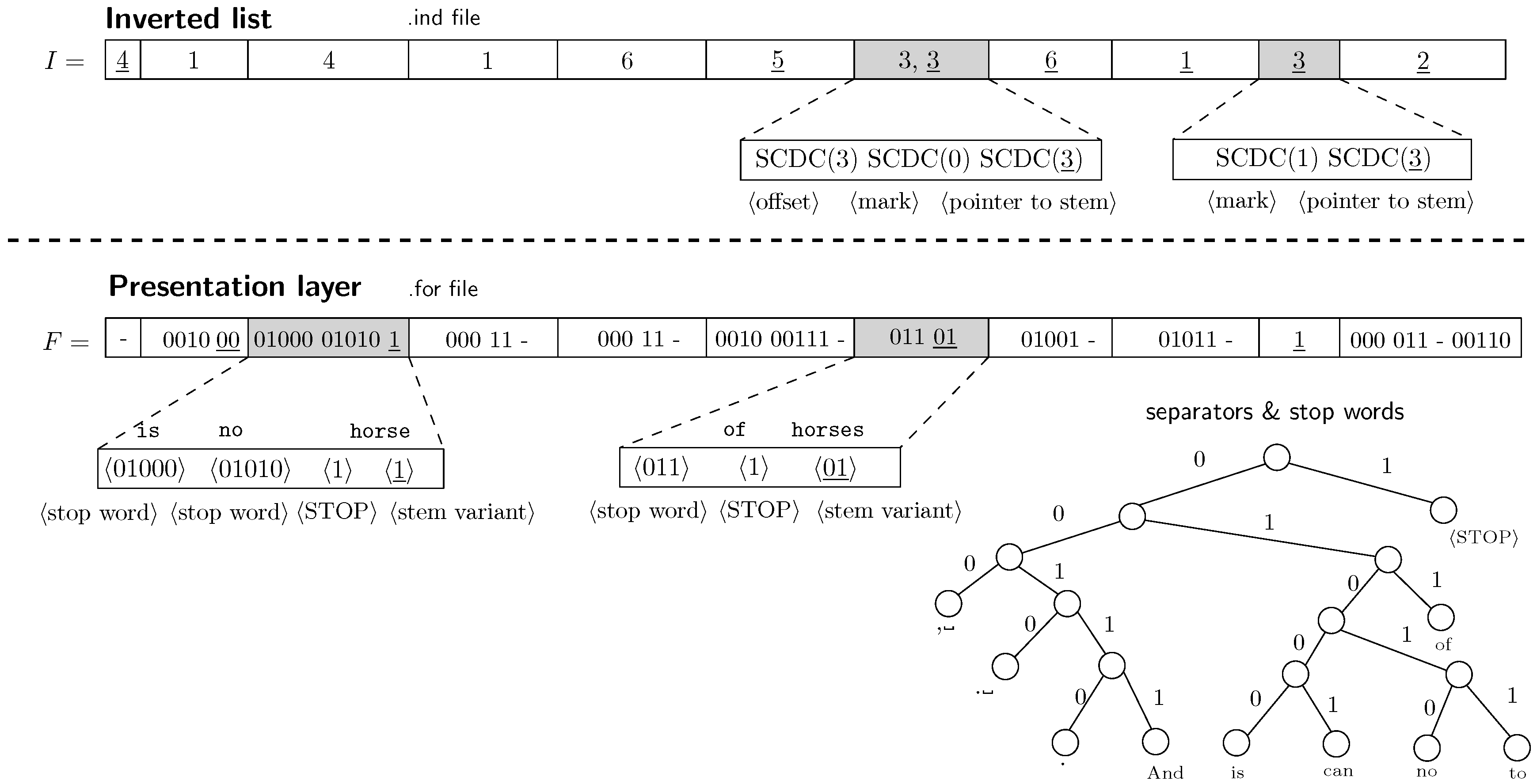
Our proposed data structure Positional Inverted Self-Index (PISI) is depicted in Figure 1. The basic idea behind PISI is to interleave the inverted lists of single terms. The inverted lists are stored as the offsets between word positions (using gap encoding). Suppose we store the offsets in the form of an arbitrary byte code. Single inverted lists can be transformed into a sequence of pointers where one occurrence points to the next one (using the offset in terms of a vector of all word positions in the processed file). Once the inverted lists are interleaved, we obtain a data structure that provides: (i) a very fast access to the sequences of single terms; (ii) a vector of all terms occurring in the processed file that can replace the file itself; (iii) the notion of a left-hand neighbour and the right-hand neighbour for each of the terms in the processed file.

The interleaved inverted list now represents the vector of term positions where a pointer at every position points to the next occurrence of the same term instead of the term position in the vocabulary. However, during the decompression process it is necessary to determine a certain word in the vector in a reasonable time. PISI inverted list (see array I) is equipped with so-called back pointers that point to the vocabulary position of the term. The period of the back pointers α represents clearly the trade-off between the size of the inverted list and the decompression speed and it means that exactly every α-th occurrence is followed by a back pointer. Finally, the last occurrence of the given term is followed by a back pointer as well.

PISI naturally undergoes all the following procedures during the construction phase. The indexed text is case folded (all letters are reduced to lower case), stopped (so-called stop words are omitted) and stemmed (all words are reduced to their stems using Porter stemming algorithm [21]). PISI uses its presentation layer (proposed by Fariña et al. [17]) to store the information lost during the aforementioned procedures. The presentation layer (see the array F) contains one (possibly empty) entry for every word of the inverted list. The entry is composed of the Huffman codes of all non-alphanumeric words and all stop words preceding the corresponding word. The entry is terminated by the Huffman code of a variant of the word (the underscored bits in the array F). The presentation layer needs to be synchronized with the inverted list (array I). PISI stores a pointer to the presentation layer for every β-th word position in the inverted list. The pointers are stored as the offset from the previous pointer in the array $\mathit{FP}$. For $\beta =3$, PISI stores the pointer for: 3rd, 6th and 9th position in the inverted list. These positions are: 6, 23 and 38. Thus, the stored offsets are: 6, 17 and 15. Furthermore, the vocabulary stores the textual representation of the stems, their word variants and the corresponding Huffman trees used for encoding of these variants. For the stems with just one variant, no Huffman tree needs to be stored and the variant is not encoded in the presentation layer either. The vocabulary also stores the common Huffman tree $T_c$ that is used to encode the non-alphanumeric words and the stop words. The next component of the vocabulary is the array $\mathit{FI}$ storing the first word positions (in the array I) of the corresponding words in the vocabulary.

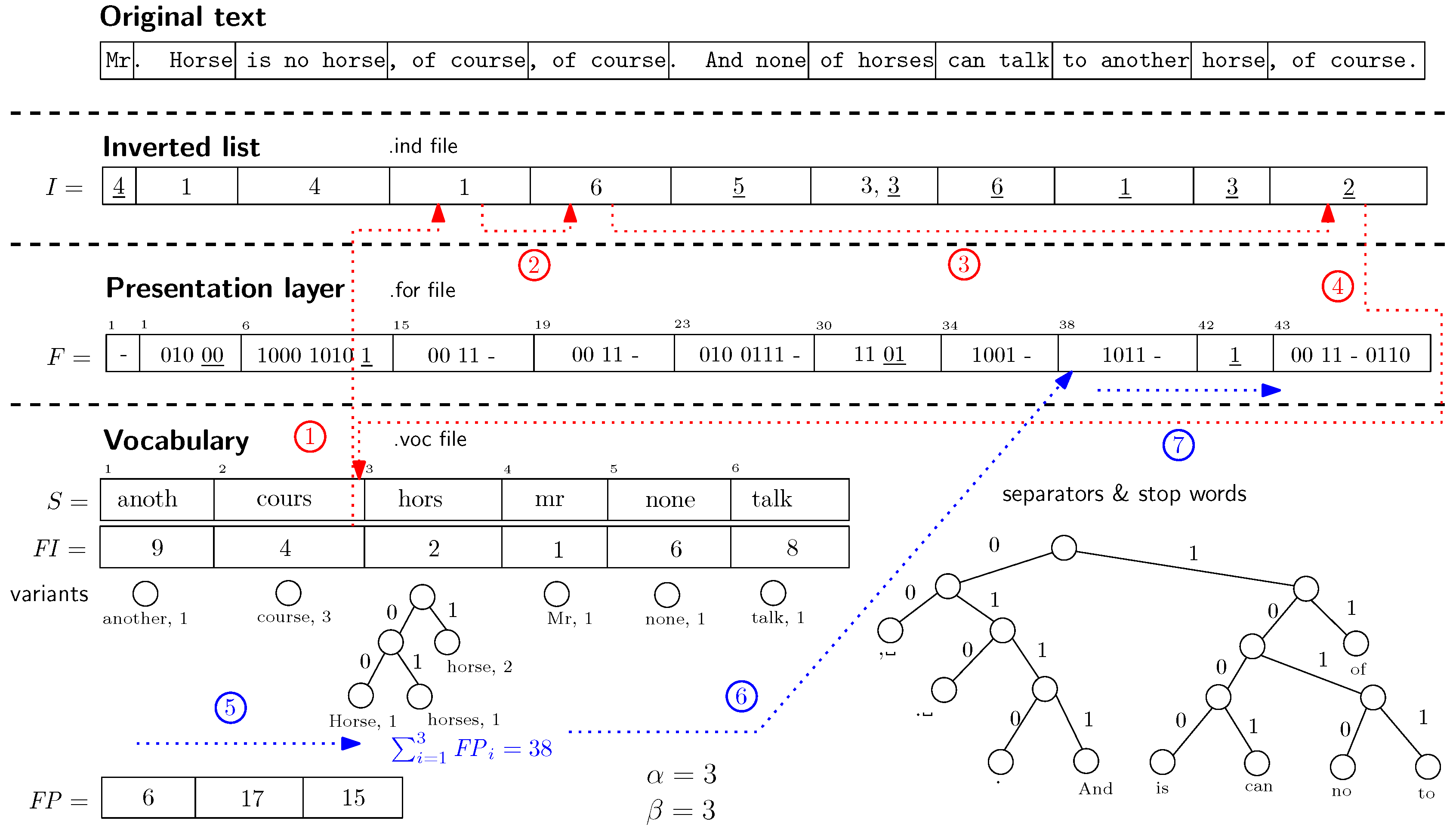
Example 1.

The dotted lines in Figure 1 describe an example of PISI search procedure. Suppose we search for the term course. First, we apply stemming on the searched term and obtain the stem cours. Next, we look for the stem in the sorted vocabulary. Once the stem is found, the algorithm starts to scan the inverted list at position ${\mathit{FI}}_2=4$ (see line ①). The algorithm jumps over the following occurrences (see lines ② and ③). Finally, the last occurrence stores a back pointer to the vocabulary (line ④). The next steps depicted in Figure 1 are described also as procedure getFPointer in Algorithm 1. Suppose we want to decompress the neighbourhood of the last occurrence of the stem cours at position 11 in the inverted list. It is necessary to synchronize the presentation layer with the occurrence in the inverted list. The previous synchronization point is at position $\lfloor \frac{11}{\beta }\rfloor =\lfloor \frac{11}{3}\rfloor =3$. The algorithm sums up the offsets stored in $\mathit{FP}$ array and it starts at position ${\sum }_{i=1}^3{\mathit{FP}}_i=38$ in presentation layer that corresponds to the 9-th entry (see lines ⑤ and ⑥). Finally, the algorithm performs decompression of the entries preceding the desired 11-th entry (line ⑦). The entry decompression is basically composed of two steps. First, looking for the stem back pointer. Second, decompression of separators and the stem variant.

Figure 2 depicts details of encoding process of the inverted list and the presentation layer. In the inverted list, we need to precede every back pointer by some reserved byte. PISI uses byte $\langle 0\rangle$ for every α-th occurrence that is not the last, and byte $\langle 1\rangle$ for the last occurrence in the sequence. The byte $\langle 0\rangle$ is preceded by a pointer to the next occurrence in the inverted list 〈offset〉 and followed by a back pointer to the vocabulary 〈pointer to stem〉. The byte $\langle 1\rangle$ is followed only by the back pointer. In the presentation layer, it is necessary to mark the end of the sequence of non-alphanumeric words and stop words. PISI uses a reserved word 〈STOP〉 that obtains the shortest Huffman code in the tree $T_c$. PISI works in so-called spaceless word model that expects the single space character ␣ as a default separator.

PISI inverted list is encoded using a byte code, particularly SCDC [19]. For the sake of efficiency, it is practical to store byte instead of word position offsets in the inverted list. The word position offsets (presented in Figure 1 and Figure 2) can be easily transformed into the byte offsets. This small change means only a negligible loss in compression ratio, however, it enables fast traversal of the inverted list of a chosen term without the need of previous preprocessing. This traversal is theoretically (not concerning the memory hierarchy of the computer) of the same speed as in the case of the standard positional inverted index.

Before we give a formal definition of PISI data structure we need to introduce some other concepts. Suppose an input text T composed of single words. T is transformed into $\widehat{T}$ using stemming, stopping and case folding. Thus, $\widehat{T}$ is a vector of length N composed of single stems extracted from T. The function ${\mathtt{rank}}_{\widehat{T}}(s,i)$ returns the number of occurrences of the stem s in the vector $\widehat{T}$ up to the position i. The function ${\mathtt{select}}_{\widehat{T}}(s,i)$ returns the position of the i-th occurrence of the stem s in the vector $\widehat{T}$ and it returns 0 if there is no such a occurrence. The function ${\mathtt{bcl}}_I(i)$ returns the length of the byte code used to encode elements of the vector I up to the position i. Now we can formally define the most important parts of PISI data structure.

Definition 1.

The PISI inverted list I is defined as a vector of length N, where N is a number of stems in $\widehat{T}$. The element $I_i$ is composed of the following components encoded using the byte code:

• mark byte $\langle 1\rangle$ when ${\widehat{T}}_i$ is the last occurrence of the stem ${\widehat{T}}_i$.
• mark byte $\langle 0\rangle$ when ${\mathtt{rank}}_{\widehat{T}}({\widehat{T}}_i,i)=k\times \alpha$, where $k\in {\mathbb{Z}}_{>0}$, i.e., ${\mathtt{rank}}_{\widehat{T}}({\widehat{T}}_i,i)$ is divisible by α and, at the same time, ${\widehat{T}}_i$ is not the last occurrence of the stem ${\widehat{T}}_i$.
• ${\mathtt{bcl}}_I({\mathtt{select}}_{\widehat{T}}({\widehat{T}}_i,{\mathtt{rank}}_{\widehat{T}}({\widehat{T}}_i,i)+1)-1)-{\mathtt{bcl}}_I(i)+1$ representing the pointer (in bytes) to the next occurrence of the stem ${\widehat{T}}_i$ in terms of the vector I when ${\widehat{T}}_i$ is not the last occurrence of the stem ${\widehat{T}}_i$.
• the pointer $S_{{\widehat{T}}_i}$ to the vocabulary representing the stem ${\widehat{T}}_i$ when ${\mathtt{rank}}_{\widehat{T}}({\widehat{T}}_i,i)=k\times \alpha$, where $k\in {\mathbb{Z}}_{>0}$, or ${\widehat{T}}_i$ is the last occurrence of the stem ${\widehat{T}}_i$.

Definition 2.

The PISI presentation layer F is defined as a vector of length N, where N is a number of stems in $\widehat{T}$. The element $F_i$ is composed of the following components encoded using the Huffman code:

• zero or more Huffman codewords representing the sequence of stop words and separators (except the single space) preceding the stem ${\widehat{T}}_i$.
• the reserved word 〈STOP〉. This component is required.
• the Huffman codeword representing a variant of the stem ${\widehat{T}}_i$. This component is included only if the stem ${\widehat{T}}_i$ has more than one variant.

Algorithm 1 describes the main functions performed by PISI. The function getStem returns a stem position in the vocabulary of a word at the position i. It basically traverses the inverted list using the pointers (see rows 22 and 26). When it reaches the reserved byte $\langle 1\rangle$ (see line 19) or the reserved byte $\langle 0\rangle$ (see line 24) it decodes and returns the following pointer to the vocabulary.

Algorithm 1 PISI Decompression from Byte Position f

1: function decompress(f, t) 2:   $\mathit{fPointer}\leftarrow$ getFPointer(f); 3:   while $f\le t$ do 4:     repeat 5:       $w\leftarrow$ Huffman decode at position $F\left[\mathit{fPointer}\right]$ using $T_c$; 6:       $\mathit{fPointer}\leftarrow \mathit{fPointer}+$ Huffman codeword length; 7:       output(w); 8:     until $w\ne \langle \mathit{STOP}\rangle$ 9:     $s\leftarrow$ getStem(f); 10:     $f\leftarrow f+$ SCDC codeword length; 11:     if $T_s$.size $>1$ then 12:       $w\leftarrow$ Huffman decode at position $F\left[\mathit{fPointer}\right]$ using $T_s$; 13:       $\mathit{fPointer}\leftarrow \mathit{fPointer}+$ Huffman codeword length; 14:     else 15:       $w\leftarrow$ the only word with the stem s; 16:     output(w); 17: function getStem(i) 18:   while TRUE do 19:     if $I\left[i\right]=1$ then 20:       $i\leftarrow i+1$; $s\leftarrow$ SCDC decode at position i; return s; 21:     else 22:       $p\leftarrow$ SCDC decode at position i; 23:       $i\leftarrow i+$ SCDC codeword length; 24:       if $I\left[i\right]=0$ then 25:        $i\leftarrow i+1$; $s\leftarrow$ SCDC decode at position i; return s; 26:     $i\leftarrow i+p$; 27: function getFPointer(i) 28:   $f\leftarrow i/\beta$; $j\leftarrow 0$; 29:   $\mathit{fPointer}\leftarrow 0$; 30:   while $j\le f$ do 31:     $\mathit{fPointer}\leftarrow \mathit{fPointer}+\mathit{FP}\left[j\right]$; $j\leftarrow j+1$; 32:   $f\leftarrow f\times \beta$; 33:   while $f<i$ do 34:     repeat 35:       $w\leftarrow$ Huffman decode at position $F\left[\mathit{fPointer}\right]$ using $T_c$; 36:       $\mathit{fPointer}\leftarrow \mathit{fPointer}+$ Huffman codeword length; 37:     until $w\ne \langle \mathit{STOP}\rangle$ 38:     $s\leftarrow$ getStem(f); $f\leftarrow f+$ SCDC codeword length; 39:     if $T_s$.size $>1$ then 40:       $w\leftarrow$ Huffman decode at position $F\left[\mathit{fPointer}\right]$ using $T_s$; 41:       $\mathit{fPointer}\leftarrow \mathit{fPointer}+$ Huffman codeword length; 42:   return $\mathit{fPointer}$;

The function getFPointer is necessary to find a position in the presentation layer F corresponding to the position i in the inverted list I. The algorithm finds the first stored $\mathit{fPointer}$ preceding the position i (see line 28). Next, the algorithm sums up offsets stored in $\mathit{FP}$ (see rows 30–31). In the next while cycle (line 33), the algorithm traverses the inverted list I and correspondingly the presentation layer F. The next repeat-until cycle (see line 34) traverses all the non-alphanumeric words and stop words preceding the word at position f. Next, the algorithm finds a stem s corresponding to the word at position f (see line 38) and decodes the word variant of the stem s (see line 40). Finally, when the actual position f in the inverted list I corresponds to i, the corresponding position in the presentation layer F is stored in $\mathit{fPointer}$.

The function decompress performs the decompression starting at position f and processing next t words. The function exactly mimics the behaviour of getFPointer function (starting from line 33). The only difference is that the function decompress outputs the decoded non-alphanumeric words and stop words of the presentation layer (see line 7) and it outputs the stem variants (see line 16). The condition at line 11 decides, whether the algorithm decodes the stem variant or it outputs the only existing stem variant.

We provide the following theorems defining the space and time complexity of PISI data structure. Theorem 1 defines the upper bound of space needed for PISI inverted list. Theorem 2 defines the upper bound of space needed for PISI presentation layer. Finally, Theorem 3 defines the upper bound of time needed to locate all occurrences of a queried term.

Theorem 1.

The upper bound for space of PISI inverted list defined by Definition 1 is $\mathcal{O}((N-n)\lceil {log}_{2^b}N\rceil +(\lfloor \frac{N-n}{\alpha }\rfloor +n)\times (\lceil {log}_{2^b}n\rceil +1))$ where N is a number of stems, n is a number of unique stems, α is a step/period of the back pointers in the inverted list and b is a size of the word of computer memory given in bits.

Proof. 

Suppose $b=8$, which implies that the following space complexities are given in bytes. Consider the PISI inverted list depicted as I array in Figure 1 and Figure 2. The inverted list I is composed of N entries. $(N-n)$ of the entries contain the pointers to the next occurrence of the stem of size $\lceil {log}_{2^b}N\rceil$. This gives the upper bound of space $\mathcal{O}((N-n)\lceil {log}_{2^b}N\rceil )$.

Suppose $N={\sum }_{i=1}^n{N}_i$ where $N_i$ represents the number of occurrences of the stem i. Furthermore, suppose $N_i=\alpha \times k_i+1$ for all $i\in \{1,..,n\}$, i.e., the number of occurrences of each stem reduced by one is divisible by α. It follows that $N-n={\sum }_{i=1}^n{N}_i-n={\sum }_{i=1}^n(\alpha \times k_i+1)-n=\alpha \times {\sum }_{i=1}^n{k}_i$. Then $N-n$ is clearly divisible by α and this composition of stem occurrences represents the maximum possible number of back pointers ${\sum }_{i=1}^n{k}_i$ for the given parameters N and n.

The sequence of the occurrences of a certain stem is always terminated by the last back pointer for each stem which means another n back pointers. Each back pointer is encoded using $\lceil {log}_{2^b}n\rceil$ bytes and it is marked by a reserved one-byte codeword ($\langle 1\rangle$ for the last back pointer and $\langle 0\rangle$ otherwise). This gives the space $\mathcal{O}((\lfloor \frac{N-n}{\alpha }\rfloor +n)\times (\lceil {log}_{2^b}n\rceil +1)))$ consumed by the back pointers. We conclude the upper bound for space needed for PISI inverted list is $\mathcal{O}((N-n)\lceil {log}_{2^b}N\rceil +(\lfloor \frac{N-n}{\alpha }\rfloor +n)\times (\lceil {log}_{2^b}n\rceil +1))$. ☐

Theorem 2.

The space needed for PISI presentation layer defined by Definition 2 is bounded by $\mathcal{O}(-{\sum }_{i=1}^N\lceil {log}_2{p}_i^{n(i)}\rceil -{\sum }_{j=1}^{N^{\prime }}\lceil {log}_2{p}_j^{\prime }\rceil +N)$ with respect to $p_i^{n(i)}$ as the probability of a stem variant at position i, $p_j^{\prime }$ as the probability of a separator or a stop word at position j and $N^{\prime }$ as the number of separators and stop words.

Proof. 

The PISI presentation layer is composed of the entries corresponding to the entries of the PISI inverted list. The number of entries is N. Every entry is terminated by a special 〈STOP〉 word followed by encoded stem variant. The presentation layer stores basically text preceding the indexed terms (stems) and the stem variants. Suppose the text surrounding the indexed terms is parsed using the space-less word-based model. Furthermore, suppose an entropy coder working with statistical model $p^{\prime }$ composed of these words (separators and stop words) and the special 〈STOP〉 word. The 〈STOP〉 is usually the most frequent word of the model and it is encoded by a constant number of bits (usually one bit). This implies $\mathcal{O}(N)$ bit needed to encode all the 〈STOP〉 words.

The number of unique stems is n and every stem stores its statistical model $p^{stem}$ of all its variants for $stem\in \{1,..,n\}$. Then $p_i^{n(i)}$ represents the probability of the stem variant at position i in terms of the statistical model of stem $n(i)$. Entropy coder encodes this variant using $-\lceil {log}_2{p}_i^{n(i)}\rceil$ bits, which implies the maximum number of $-{\sum }_{i=1}^N\lceil {log}_2{p}_i^{n(i)}\rceil$ bits necessary to encode all stem variants. It is easy to see that the entropy coder encodes $N^{\prime }$ separators using $-{\sum }_{j=1}^{N^{\prime }}\lceil {log}_2{p}_j^{\prime }\rceil$ bits where $p_j^{\prime }$ represents a probability of the j-th separator. We conclude that the number of bits needed to encode PISI presentation layer is bounded above by $\mathcal{O}(-{\sum }_{i=1}^N\lceil {log}_2{p}_i^{n(i)}\rceil -{\sum }_{j=1}^{N^{\prime }}\lceil {log}_2{p}_j^{\prime }\rceil +N)$. ☐

Theorem 3.

The PISI ensures the operation locate in worst-case time $\mathcal{O}(\lfloor \frac{N}{\beta }\rfloor +occ\times \beta \times \alpha )$ where $occ$ is the number of occurrences of a queried term, α is the step/period of the back pointers in the inverted list and β is the step/period of the synchronization points synchronizing the inverted list with the presentation layer.

Proof. 

The simple structure of PISI inverted list ensures that it can be traversed in $occ$ steps. To determine a position of a term and possibly decompress its neighbourhood it is necessary to synchronize every occurrence with the presentation layer. The synchronization points are stored as the offsets in $\mathit{FP}$ array and ${\sum }_{i=1}^k{\mathit{FP}}_i$ represents a position of the entry corresponding to the stem at position $k\times \beta$ in the inverted list. Suppose the search performed from left to right and the achieved synchronization points are cached during the search. Then the time needed for summation of all necessary synchronization points is bounded by $\mathcal{O}(\lfloor \frac{N}{\beta }\rfloor )$.

One has to decompress β entries from the corresponding synchronization point to achieve a position of the wanted term in the worst case. Decompressing of one entry is composed of two steps. First, to determine the stem. Second, to decompress the separators preceding the stem and decompress the stem variant. Suppose the encoded separators, stem variants and the gaps can be decoded in the constant time. Then the first step can be performed in $\alpha \times \mathcal{O}(1)$ in the worst case. The second step can be done in $\mathcal{O}(1)$ time considering standard natural language text with a low constant number of separators between two following stems. Thus, locating one occurrence takes $\mathcal{O}(\beta \times \alpha )$ time. We conclude that the time needed to locate all occurrences of one term is bounded above by $\mathcal{O}(occ+\lfloor \frac{N}{\beta }\rfloor +occ\times \beta \times \alpha )=\mathcal{O}(\lfloor \frac{N}{\beta }\rfloor +occ\times \beta \times \alpha )$. ☐

3.1. The Context of PISI Implementation

Suppose an IR system that uses positional ranking function to score the documents and that extracts snippets for top-scoring documents. According to [16], the evaluation of a query involves the following steps:

• Query Processing Step: Retrieve top-$k_1$ scoring documents according to some standard document ranking function and the given query.
• Positional Ranking Step: Rerank the top-$k_1$ documents according to some positional ranking function and the positions of the query terms.
• Snippet Generation Step: Generate snippet for top-$k_2$ documents where $k_2\le k_1$.

PISI addresses the second and the third step of the aforementioned scenario. In the second step, PISI uses the information about the positions of single words. In the third step, PISI is rewarded for its high decompression speed. For the first step, some traditional (document-level) inverted index must be applied since this step is performed on a very large number of documents.

It implies that, in real implementations, PISI needs to cooperate at least with a standard (document-level) inverted index. The implementation of such a framework is out of the scope of this paper. However, we outline at least the concept of the framework in the following example.

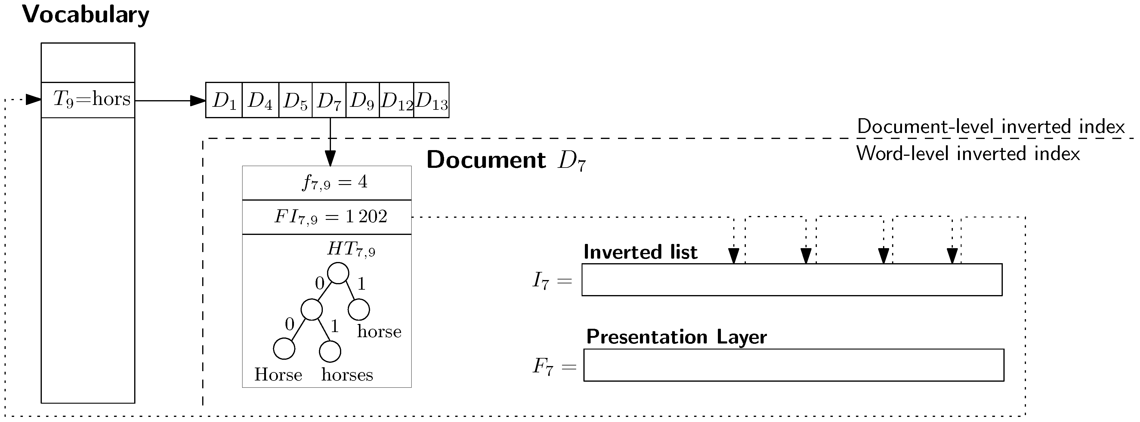
Example 2.

Figure 3 depicts an example of the integration of the standard inverted index with PISI. Both inverted indexes share the vocabulary storing the stems of single words. The vocabulary is alphabetically sorted and except the textual representation of the stem it stores also a pointer to inverted list with documents IDs. Every slot of the inverted list corresponding to a document contains frequency of the given word in the given document $f_{d,t}$, pointer to the first occurrence of the word $F{I}_{d,t}$ and the Huffman tree $H{T}_{d,t}$ storing concrete variants of the stem.

We can observe in Figure 3 that the stem “hors” occurs i.a. in the document $D_7$. The document $D_7$ contains $f_{7,9}=4$ occurrences of the stem in the tree different variants (see the Huffman tree $H{T}_{7,9}$). The first occurrence is at the position $F{I}_{7,9}=1202$. The last position of the stem stores a back pointer to the vocabulary entry $T_9$. The dashed line determines a border between the two components: standard (document-level) inverted index and the word-level inverted index (PISI).

4. Experiments

We designed our experiments with respect to the two main questions we asked. What is the performance of PISI compared to the word-based self-indexes proposed by Fariña et al. in [17]? What is the difference in the search speed of PISI compared to standard positional inverted index?

Thanks to the space limits we focus especially on the first question in this paper. To the second question, we can briefly mention that PISI pays for breaking of locality of the stored inverted lists. Depending on the cache size of the computer, PISI can be up to five times slower in searching than the standard positional inverted index.

We carried out our tests on Intel^® Core^TM i7-4702MQ $2.20$ GHz, 8 GB RAM. We used compiler gcc version 4.9.3 with compiler optimization -O3.

All reported times represent measured user time + sys time. All our experiments run entirely in RAM. All the reported experiments were performed on bible.txt file of the Canterbury corpus.

The first experiment provides a space breakdown of PISI into the single components of the index data structure. Different instances of PISI are stated in the single columns of

Table 1. PISI space breakdown when performed on bible.txt file. The space is given in bytes (memory consumption in upper part of the table and the disk storage consumption in lower part of the table). The compression ratio refers to size of the original file.

Parameters		α	10	10	15	20	40	80	100	120
		β	20	40	40	40	80	100	100	100
MEMORY	.ind file	gaps	$\mathrm{582,901}$	$\mathrm{582,901}$	$\mathrm{578,919}$	$\mathrm{576,872}$	$\mathrm{573,801}$	$\mathrm{572,282}$	$\mathrm{571,961}$	$\mathrm{571,808}$
		reserved bytes	$\mathrm{42,945}$	$\mathrm{42,945}$	$\mathrm{31,128}$	$\mathrm{25,252}$	$\mathrm{16,671}$	$\mathrm{12,538}$	$\mathrm{11,769}$	$\mathrm{11,252}$
		back pointers	$\mathrm{85,387}$	$\mathrm{85,387}$	$\mathrm{61,864}$	$\mathrm{50,167}$	$\mathrm{33,086}$	$\mathrm{24,857}$	$\mathrm{23,327}$	$\mathrm{22,297}$
	.for file	stoppers	$\mathrm{46,233}$	$\mathrm{46,233}$	$\mathrm{46,233}$	$\mathrm{46,233}$	$\mathrm{46,233}$	$\mathrm{46,233}$	$\mathrm{46,233}$	$\mathrm{46,233}$
		stem variants	$\mathrm{42,598}$	$\mathrm{42,598}$	$\mathrm{42,598}$	$\mathrm{42,598}$	$\mathrm{42,598}$	$\mathrm{42,598}$	$\mathrm{42,598}$	$\mathrm{42,598}$
		NAN words	$\mathrm{82,541}$	$\mathrm{82,541}$	$\mathrm{82,541}$	$\mathrm{82,541}$	$\mathrm{82,541}$	$\mathrm{82,541}$	$\mathrm{82,541}$	$\mathrm{82,541}$
		stop words	$\mathrm{334,933}$	$\mathrm{334,933}$	$\mathrm{334,933}$	$\mathrm{334,933}$	$\mathrm{334,933}$	$\mathrm{334,933}$	$\mathrm{334,933}$	$\mathrm{334,933}$
	.voc file	words	$\mathrm{175,933}$	$\mathrm{175,933}$	$\mathrm{175,933}$	$\mathrm{175,933}$	$\mathrm{175,933}$	$\mathrm{175,933}$	$\mathrm{175,933}$	$\mathrm{175,933}$
		Huffman trees	$\mathrm{246,820}$	$\mathrm{246,820}$	$\mathrm{246,820}$	$\mathrm{246,820}$	$\mathrm{246,820}$	$\mathrm{246,820}$	$\mathrm{246,820}$	$\mathrm{246,820}$
		$\mathit{FP}$	$\mathrm{35,756}$	$\mathrm{23,571}$	$\mathrm{23,571}$	$\mathrm{23,585}$	$\mathrm{15,576}$	$\mathrm{12,189}$	$\mathrm{12,189}$	$\mathrm{12,189}$
		sorted stems	$\mathrm{36,836}$	$\mathrm{36,836}$	$\mathrm{36,836}$	$\mathrm{36,836}$	$\mathrm{36,836}$	$\mathrm{36,836}$	$\mathrm{36,836}$	$\mathrm{36,836}$
		$\mathit{FI}$	$\mathrm{36,836}$	$\mathrm{36,836}$	$\mathrm{36,836}$	$\mathrm{36,836}$	$\mathrm{36,836}$	$\mathrm{36,836}$	$\mathrm{36,836}$	$\mathrm{36,836}$
	total		$\mathrm{1,749,719}$	$\mathrm{1,737,534}$	$\mathrm{1,698,212}$	$\mathrm{1,678,606}$	$\mathrm{1,641,864}$	$\mathrm{1,624,596}$	$\mathrm{1,621,976}$	$\mathrm{1,620,276}$
	compression ratio		$42.91$	$42.61$	$41.65$	$41.16$	$40.26$	$39.84$	$39.78$	$39.73$
SERIALIZED	.ind file		$\mathrm{711,233}$	$\mathrm{711,233}$	$\mathrm{671,911}$	$\mathrm{652,291}$	$\mathrm{623,558}$	$\mathrm{609,677}$	$\mathrm{607,057}$	$\mathrm{605,357}$
	.for file		$\mathrm{506,306}$	$\mathrm{506,306}$	$\mathrm{506,306}$	$\mathrm{506,306}$	$\mathrm{506,306}$	$\mathrm{506,306}$	$\mathrm{506,306}$	$\mathrm{506,306}$
	.voc file		$\mathrm{180,365}$	$\mathrm{168,200}$	$\mathrm{168,137}$	$\mathrm{168,188}$	$\mathrm{160,151}$	$\mathrm{156,748}$	$\mathrm{156,694}$	$\mathrm{156,659}$
	total		$\mathrm{1,397,904}$	$\mathrm{1,385,739}$	$\mathrm{1,346,354}$	$\mathrm{1,326,785}$	$\mathrm{1,290,015}$	$\mathrm{1,272,731}$	$\mathrm{1,270,057}$	$\mathrm{1,268,322}$
	compression ratio		$34.28$	$33.98$	$33.02$	$32.54$	$31.64$	$31.21$	$31.15$	$31.10$

according to setting of the parameters α (the period of the back pointers) and β (the period of the pointers synchronizing inverted list with the presentation layer). Higher values of both parameters mean better compression ratio but slower decompression. The growing parameter α reduces the number of the back pointers as well as the reserved bytes. The omitted back pointers cause shorter gaps and thus shorter encoding of the gaps. The parameter β influences only the array $\mathit{FP}$ which stores the pointers to the presentation layer. Table 1 shows also the space difference between the memory consumption (upper part of the table) and disk storage consumption (lower part of the table). It can be seen that the serialization influences only the vocabulary (.voc file). In the serialized form, the stem variants are encoded only as the suffix extending the stem and the Huffman trees are encoded as simple bit vectors.

We demonstrate the effect of the parameters α and β on the compression ratio and the snippet time in Figure 4. Generally, we can observe that the parameter β has lower impact on the compression ratio and the snippet time than the parameter α. Only the size of $FP$ array is influenced by β and it is not crucial in terms of the total size of PISI data structure. On the other hand, β impacts the search and decompression process only at one point when the presentation layer F has to be synchronized with the inverted list I. Thus, lower values of β (i.e., shorter distances between the two following synchronization points) provide only limited gain in terms of the snippet time. Figure 4 proves that the parameter α significantly impacts the snippet time at the expense of small increase of the necessary space. This pays approximately up to the value $\alpha =20$ when PISI encounters its speed limits. Further increment of α brings only negligible improvements of the snippet time together with a significant increase of the compression ratio.

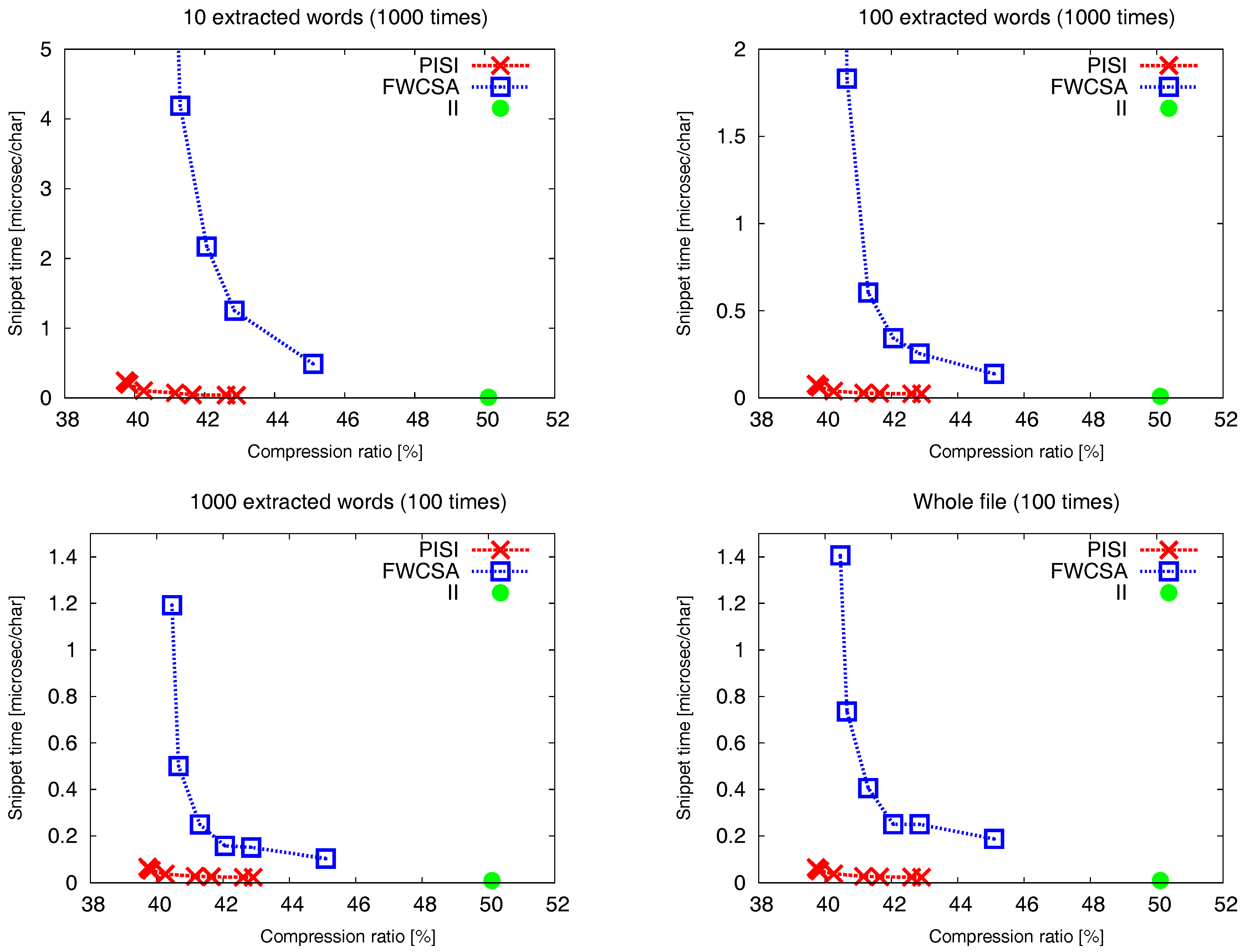
Figure 5 shows a trade-off between the compression ratio and the time needed to extract a snippet. The snippet time includes search time and a time needed to extract a certain number of words (10, 100, 1000 and the whole file). We tested so-called bag-of-words search with four words randomly chosen of the indexed text. We compare three different indexes: our PISI, word-based self-index FWCSA proposed by Fariña et al. in [17] and the standard positional inverted index II. II is our implementation and it uses SCDC encoded inverted lists. The text accompanying the index is SCDC encoded, as well. All the parameters of FWCSA were set to power of two ensuring the highest possible speed. Disregarding the number of extracted words, all the presented charts show very similar curves. The standard positional inverted index (II) provides the best snippet time ($9.51\times {10}^{-9}$ second per extracted character for 1000 extracted words). However, the inverted index together with the compressed file (which cannot be replaced) achieve the worst compression ratio $50.11$%. The fastest instance of PISI with achieved compression ratio $42.91$% proved to be 2–3 times slower than II (with snippet time $2.37\times {10}^{-8}$ s per extracted character for 1000 extracted words). Furthermore, PISI proved to achieve usually an order of magnitude better snippet time at some level of compression ratio in comparison to FWCSA, e.g., PISI with compression ratio $42.91$% achieves snippet time $3.84\times {10}^{-8}$ s per extracted character for 10 extracted words. On the other hand, FWCSA with compression ratio $42.85$% achieves snippet time $1.25\times {10}^{-6}$ s per extracted character for 10 extracted words. Finally, PISI is able to achieve the best compression ratio among of all tested algorithms, which is $39.73$%.

5. Conclusions and Future Work

We responded the challenge impelling to higher effectiveness in storage of positional inverted indexes. Our proposal PISI represents the idea of self-indexing based on a simple positional inverted index. It reduces a lack of effectiveness of the positional inverted index and at the same time it exploits high processing speed and simplicity of inverted indexing. We compared PISI with its closest competitors FWCSA and the standard positional inverted index II. PISI proved to overcome the standard inverted index in the compression ratio and FWCSA in the search and decompression speed.

We state the following points of our future work:

• We intend to further test this version of PISI on TREC corpora. We will give the needed optimizations for larger data sets, if necessary.
• We want to present a broader comparison with other relative compressed data structures, e.g., other variants of standard positional inverted index.
• We aim to give a comparison of our way of compressing the presentation layer with the way used by FWCSA when the whole text occurring between two following stems is considered as a single separator.
• We plan to implement a framework integrating PISI with the standard (document-level) inverted index and perform experiments that involve all three steps of the search process (mentioned in Section 3.1) and that correspond to the searching in some real search engine.