
A Spatial-Temporal-Semantic Neural Network Algorithm for Location Prediction on Moving Objects


1
Key Laboratory of Spatial Information Precessing and Application System Technology, Institude of Electronics, Chinese Academy of Sciences, Beijing 100190, China
2
School of Electronic, Electrical and Communication Engineering, University of Chinese Academy of Sciences, Beijing 100190, China
*
Author to whom correspondence should be addressed.
Algorithms 2017, 10(2), 37; https://doi.org/10.3390/a10020037
Submission received: 20 February 2017
/
Revised: 21 March 2017
/
Accepted: 22 March 2017
/
Published: 24 March 2017
Abstract
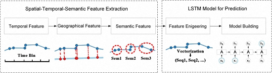
:Location prediction has attracted much attention due to its important role in many location-based services, such as food delivery, taxi-service, real-time bus system, and advertisement posting. Traditional prediction methods often cluster track points into regions and mine movement patterns within the regions. Such methods lose information of points along the road and cannot meet the demand of specific services. Moreover, traditional methods utilizing classic models may not perform well with long location sequences. In this paper, a spatial-temporal-semantic neural network algorithm (STS-LSTM) has been proposed, which includes two steps. First, the spatial-temporal-semantic feature extraction algorithm (STS) is used to convert the trajectory to location sequences with fixed and discrete points in the road networks. The method can take advantage of points along the road and can transform trajectory into model-friendly sequences. Then, a long short-term memory (LSTM)-based model is constructed to make further predictions, which can better deal with long location sequences. Experimental results on two real-world datasets show that STS-LSTM has stable and higher prediction accuracy over traditional feature extraction and model building methods, and the application scenarios of the algorithm are illustrated.
1. Introduction
With the rapid growth of positioning technology, locations can be acquired by many devices such as mobile phones and global position system (GPS)-based equipment. Location prediction is of great significance in many location-based services. For example, while a package is being delivered, customers are eager to know where the courier is and which place he would visit next, in order to estimate the arrival time of the package. The same scenario applies to food delivery. Moreover, in public transportation systems, passengers are curious about where the nearest taxi or bus will go so as to estimate their waiting time. In real-time advertising systems, places where customers will go are important because they determine which kinds of ads to be posted. Location prediction can be determined in the following way: given a series of locations, pre-collected or real-time-dependent, location prediction techniques will infer the next location where the object is most likely to go.
Due to the continuity of space and time, trajectory is not suitable to be directly imported to a prediction model. Before using prediction models, each of the points in a trajectory is first preprocessed in order to convert the real continuous values associated to the geospatial coordinates of latitude and longitude, into discrete codes associated to specific regions. Traditional prediction methods usually start with clustering trajectories into frequent regions or stay points, or simply partition trajectories into cells. Trajectories are transformed into clusters or grids with discrete codes, then pattern mining or model building techniques are utilized to find frequent patterns along the clusters. For example, the historical trajectories of a person show that he always go to the restaurant after the gym. If the person is now in the gym, it is a distinct possibility that the next place he will visit is the restaurant.
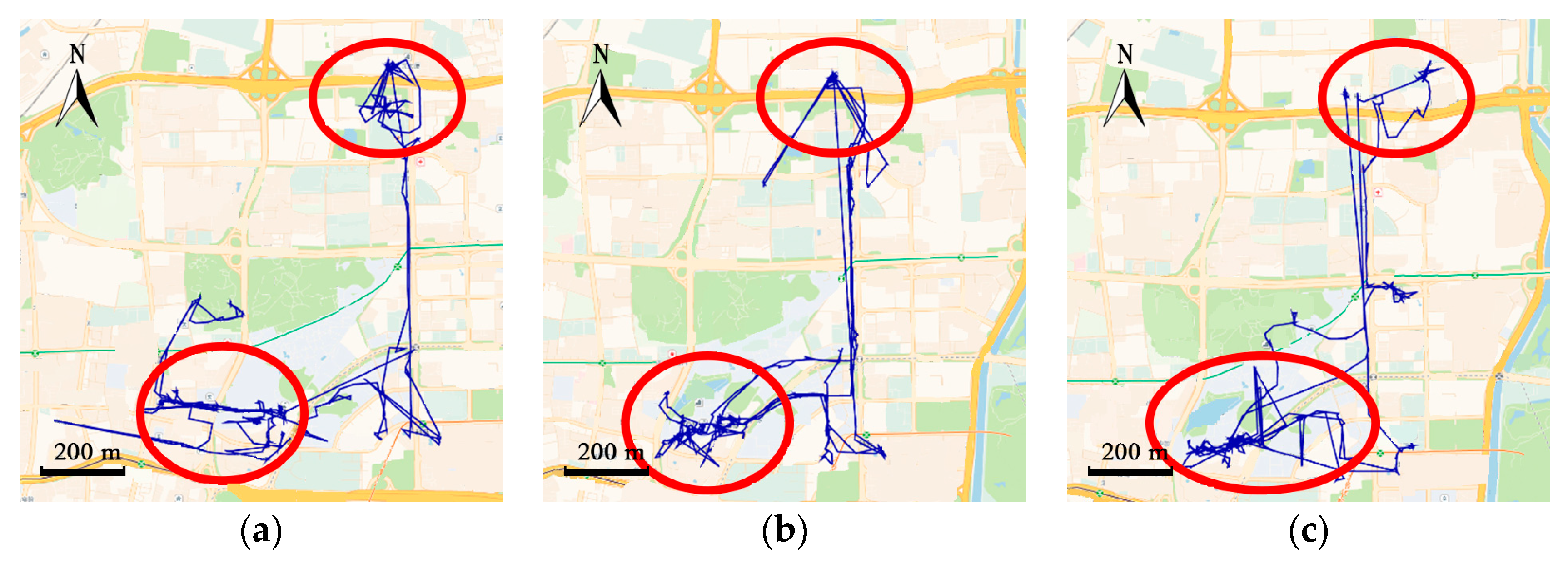
However, traditional cluster-based or cell-based methods ignore trajectories between the clusters, which may contain critical information for specific applications. For example, trajectories in Figure 1a contain 350 track points and only two frequent regions are grouped. Traditional methods can infer region 2 from region 1, but fail to predict where the courier is between the two regions. Many location-based services such as delivery-pickup system and transportation system pay significant attention to predicting where the objects exactly are along the road.
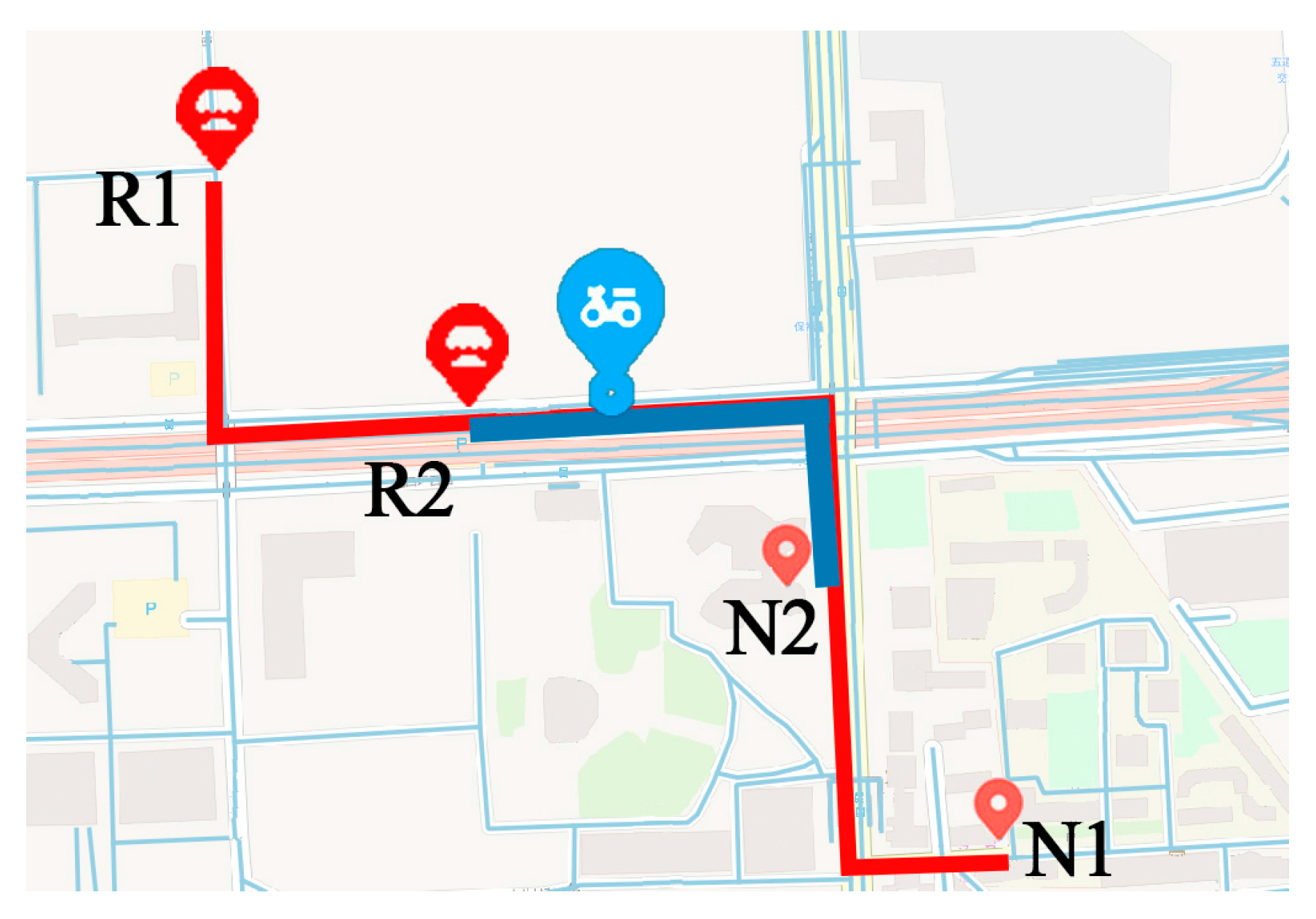
Moreover, frequent patterns or location sequences generated by clustering method are relatively short. Traditional models, such as the hidden Markov model (HMM) and the recurrent neural networks (RNN), are good at handling short sequences. However, when considering points along the road, the length of location sequences generated from raw trajectories become longer. Performance of traditional models may decline with long sequences. For example, as shown in Figure 2, the courier has two frequent patterns. He always goes to Neighborhood 1 from Restaurant 1 by the route in red, and goes to Neighborhood 2 from Restaurant 2 by the route in blue. One day he started from Restaurant 1 and traveled at the blue spot. Traditional models that deal with short sequences may suggest that the courier started from Restaurant 2, because it is not far away from the courier. Then the model will predict that the next location of the courier is Neighborhood 2 according to the historical patterns. However, the courier is actually going to Neighborhood 1.
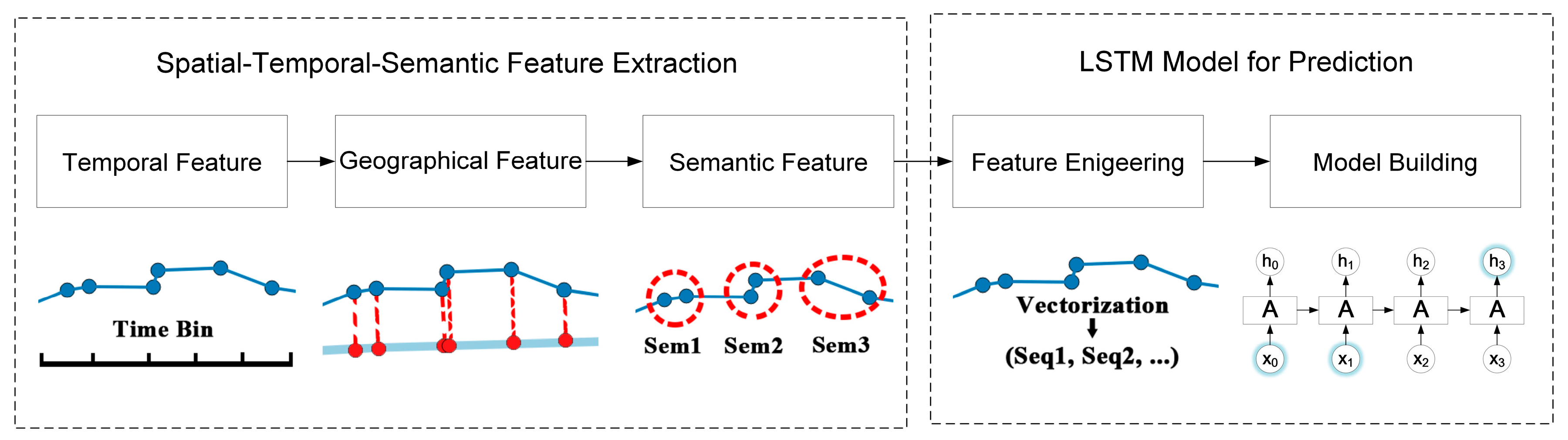
To overcome the above limitations, a spatial-temporal-semantic neural network algorithm for location prediction (STS-LSTM) is proposed in this paper. First, a spatial-temporal-semantic (STS) feature extraction algorithm is put forward to transform the whole trajectory into discrete location sequences with fixed code that are friendly to the prediction model, and will maintain points along the road; Second, a long short-term memory (LSTM)-based neural network model is proposed. The location sequences are partitioned into multiple sequences with fixed length by a sliding window. The next locations are used as labels for classification. Then, both the historical and the current trajectories are used to train the model and to make predictions. The algorithm is evaluated on two real-world datasets and compared with several classic algorithms from the aspects of both feature extraction and model building. The main novelties of the proposed algorithm and contributions of this paper are listed as follows:
- Traditional clustering-based prediction algorithms ignore trajectories between the clusters such as points along the road. The proposed STS feature extraction algorithm transforms the trajectory into location sequences with fixed and discrete road IDs. The method can take points along the road into account, which can meet the demand of specific applications. Moreover, the generated location sequences can be better used in the prediction model, which can achieve better prediction results.
- The location sequences generated by the STS feature extraction algorithm might be very long. Traditional sequential models such as HMM and RNN may not perform well with long sequences. The LSTM-based prediction model is proposed to solve the problem. The model can take advantage of location sequences over a long period of time, which can make better predictions. Evaluation results prove that both the STS feature extraction algorithm and the LSTM based prediction model outperform traditional methods.
2. Related Work
Studies on location prediction have gained increasing popularity. The most direct manner is to derive the next location by speed and direction according to the past locations. This may not be an accurate method, because the next location is affected by various factors such as traffic condition, weather, and the behaviors of the objects. In recent years, many location prediction methods focus on mining historical track data. The movements of individuals may show regularity. For example, in Figure 1, couriers deliver the packages from one neighborhood to another, following the same routes and visiting orders every day. Buses travel along the same routes every day. The combination of historical movements and the latest few locations of the objects can provide accurate prediction result.
In addition to trajectory data, location prediction methods based on other spatial-temporal data such as check in data and event-triggered data are also valuable as references. Related works in the area of location prediction are summarized in Table 1.
The next location is highly related to the interest and intentions of an object. Recommendation algorithms are used to find the most possible place the user is interested in visiting. The matrix factorization-based method by Koren [1] factorizes a user-item rating matrix considering multiple features including the geo-location. Xiong [2] extended it as tensor factorization (TF) to be time-aware, by treating time bins as another dimension when factorizing. Zheng [3] modeled spatial information into factorization models. Moreover, Bahadori [4] included both temporal and spatial aspects in TF as two separated dimensions and make location more predictable. Zhuang [5] proposed a recommender that leverages rich context signals from mobile device such as geo-location and time. However, it is hard for factorization-based models to generate movements that have never or seldom appeared in the training data. Monereale [6] proposed a hybrid method considering both the user’s own data and crowds that have similar behaviors. Recommendation-based algorithms do not consider current locations of users and the order of the movements, which may lead to a low precision of prediction.
Movement pattern mining techniques find the regularity of movements of objects and combine current movements with historical data for prediction. By transforming trajectories into cells, Jiang [7] studied trajectories of taxis and found they move in flight behaviors. Jeung [8] forecasted the future locations of a user by predefined motion functions and linear or nonlinear models, then movement patterns are extracted by an a priori algorithm. Yavas [9] utilized an improved a priori algorithm to find association rules with support and confidence. These frequent patterns reveal the co-occurrences of locations. Morzy [10] developed a modified PrefixSpan algorithm to discover both the relevance of locations and the order of location sequences. Moreover, sequential pattern methods can be improved by adding temporal information. Giannotti [11] extended travel time to location sequences and generated spatial-temporal patterns. Li [12,13] proposed two kinds of trajectory patterns: the periodic behavior pattern and the swarm pattern. Trajectories are first clustered into reference spots and a Fourier-based algorithm is utilized to detect period. Then periodic patterns are mined by hierarchical clustering. The core step of pattern-based prediction methods is to cluster frequent places. However, due to the limitation of positioning devices, track points will be lost when the satellite signal is low. For example, when buses travel into tunnels or regions covered with tall buildings, the GPS signal is blocked and no points will be collected during that time, which causes the data sparsity problem during clustering. As shown in Figure 1, the courier also frequently visited the place at the bottom-right section of the map, which is not clustered. Only two frequent areas are gathered and trajectories between the frequent regions are abandoned. Clustering-based algorithms may lose a lot of information, leading to low coverage of prediction.
After extracting the frequent regions from raw trajectories, various kinds of models can be used to make prediction. Lathia [14] proposed a time-aware neighborhood-based model paying more attention to recent locations and less to the past. Cheng [15] proposed a multi-center Gaussian model to calculate the distance between patterns. However, neighborhood-based methods do not consider the sequential factors in user’s behaviors. The Markov chain (MC) model can take sequential features into consideration. Rendle [16] extended the MC with factorization of the transition matrix and calculated the probability of each behavior based on the past behaviors. Mathew [17] proposed a hybrid hidden Markov model (HMM) to transform the trajectory into clusters and train the HMM with them. Jeung [18] transferred trajectories into frequent regions by a cell partition algorithm, treating them as hidden states and observable states of the HMM. Accuracy of the prediction depends highly on the level of granularity of the cells. For example, in Figure 3, partition by large cells is more precise and the clusters are closed to the actual boundaries of the neighborhoods. However, partition by the smaller cell loses the geo-information of the neighborhoods.
Semantically-based prediction methods claim that many behaviors of users are semantically-triggered. Alvares [19] discovered stops from trajectories and map these stops to semantic landmarks. Then a sequential pattern mining algorithm is used to achieve frequent semantic patterns. Bogorny [20] utilized a hierarchical method to obtain geographic and semantic features from trajectories. Ying [21] proposed a geographic-temporal-semantic pattern mining method for prediction, which also transforms trajectory into stay points. Then trajectory patterns are clustered to build the frequent pattern tree for detecting future movements. Semantically-based methods mainly focus on mining the stay points. The trajectories along the road are abandoned.
Recently, recurrent neural networks (RNNs) have gained a breakthrough in sequence mining. Mikolov [23] developed RNNs in word embedding for sentence modeling. Multiple hidden layers in RNN can adjust dynamically with the input of behavioral history, therefore, an RNN is suitable for modeling temporal sequence. Liu [22] extended traditional RNN with geographical and temporal contexts to handle prediction problem of spatial-temporal data. An RNN performs well with short location sequences, such as clusters and stay points. However, when considering the whole trajectory, the location sequences become longer and the precision of prediction of RNN may decline.
In conclusion, in order to utilize machine learning models, the trajectory should be transformed to be model-friendly. Existing location prediction algorithms usually cluster trajectory into cells, regions, or stay points. Track points along the road are abandoned, but these points can be important to specific applications. To solve this problem, a spatial-temporal-semantic neural network algorithm for location prediction is proposed in this paper. First, in order to transform the whole trajectory into location sequences friendly to the prediction model, STS feature extraction is utilized to map trajectory to the reference points and maintain as much information as possible; Second, the LSTM model is built to handle the long sequences generated before, and to make further prediction.
3. Methodology
The core idea of location prediction algorithms is to model regular patterns hidden in historical data and find the most possible movements based on current observations. Due to the continuity of space and time, trajectory is not suitable to be directly imported to a prediction model. As shown in Figure 4, the courier travels along the same road every day, but the trajectories are not exactly the same. Simply representing a location by continuous coordinates may lead to high computational cost and may not achieve a better prediction result. Before using prediction models, each of the points in a trajectory is first preprocessed in order to convert the real continuous values associated to the geospatial coordinates of latitude and longitude, into discrete codes associated to specific regions. Existing methods use clustering-based algorithms to transform trajectory into discrete cells, clusters and stay points. However, the density of points on the road may be relatively low compared to frequent regions, making it hard for clustering algorithm to identify. Additionally, they cannot deal with points along the road.
In Section 3.1, a spatial-temporal-semantic feature extraction algorithm is proposed to overcome the difficulties and to discretize trajectory into location sequences, namely, . As shown in Equation (1), given an object and current time , the problem of location prediction can be formulated as estimating the probability of the next location based on the current locations :
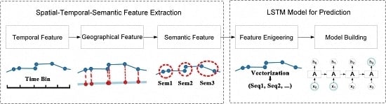
Then location prediction with discrete locations is like the classification problem. During the model building process, location sequence is used as features and is the label. However, generated by the first step might be very long and the performance of traditional models, such as HMM and RNN, will decline. In Section 3.2, a LSTM-based prediction model is proposed to handle long sequences. The flowchart of the STS-LSTM is illustrated in Figure 5.
3.1. Spatial-Temporal-Semantic Feature Extraction
A trajectory is composed of a series of track points, expressed as , where N is the number of track points. Each track point is composed of spatial information such as longitude, latitude and time stamp, expressed as , which is continuous in space and time. To discretize the trajectory, both spatial and temporal factors should be added into the model. The feature extraction method introduced in this section aims to transform the trajectory to fixed, discrete location sequences without losing much information.
3.1.1. Temporal Feature Matching
To transform continuous temporal information into discrete time, a proper time interval should be selected. Positioning devices such as the GPS module inside the mobile phone collect track points at a fixed sampling rate, usually one every second. However, due to the cost of network transmission and storage problems, points collected are not completely uploaded to the server. For example, the locations of couriers are sent to the server every five seconds and it changes to 30 s in the applications of taxi or bus. The precision of location prediction is affected by the sampling rate. If the time interval between each location is five minutes, the model will predict the next location five minutes from the current one. The time interval is determined by the demand of specific services. Generally, the time interval should be larger than the average sample rate.
Trajectories are usually stored and segmented by natural day. However, the record of tracks may be interrupted because of the GPS blocking problem. First, each trajectory is divided into segments if the time interval between two track points is over 30 min. Intervals under 30 min can be regarded as blocking, which does not affect the continuity of trajectory. After segmentation, track points are allocated to timebins. Time of a day is divided into multiple time bins by the size the time bin. For example, if the size of time bin is 15 min, there is four time bins in an hour and 144 time bins in a day, identified from 0 to 143. Next, time of each track points is mapped to a time bin by Equation (2), where is the time of . is the zero time of a day and is the integral function:
The temporal mapping process is illustrated in Figure 6. After mapping, there might be several points in the same time bin. A representative point is selected by calculating the linear center of the points with the average longitude and latitude.
Trajectory is transformed into , where is the representative point in each time bin. The sequence of representative points is sorted in ascending order of the time bin ID. After time matching, temporal information is fixed and discretized.
3.1.2. Geographical Feature Matching
Same as time factor, the geographical information of trajectory such as coordinate is continuous in space, which is difficult to use in a model. Trajectory should be converted to fixed reference points. Existing methods utilizing cell-based partitioning, clustering, and stop point detection cannot handle points on the road. Therefore, a new geographical feature mapping method is proposed to transform all the points in a trajectory. Objects always travel along the road in the city, therefore, the city road networks are selected as reference points. Open Street Map (OSM) is a project that creates and distributes free geographic data for the world [24]. Map data from OSM is in format. It contains all elements including points of interest, roads, and regions, as shown in Figure 7.
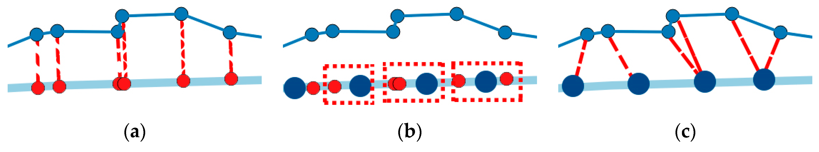
Each road can be represented as a line , with a start node and an end node . First, for each track point , find the nearest line by sorting the distance from to all lines in the network. The searching could be time consuming when the network is very large. However, with the indexing technology used in geo-database such as PostgreSQL, the process could be executed in milliseconds. The projection point of on is calculated by Equation (3), shown as the red points in Figure 8a, where is the slope of :
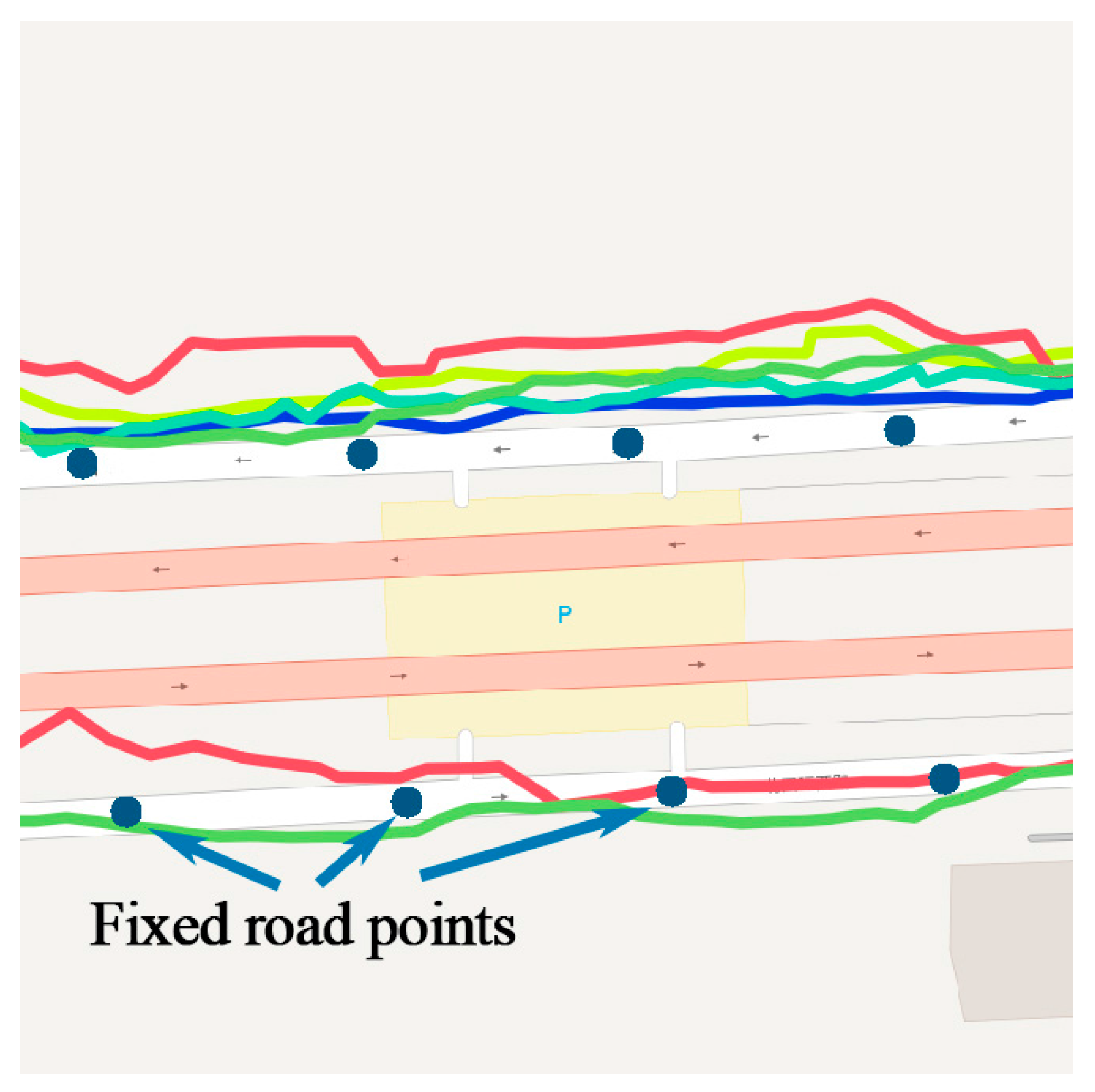
The projection point could be anywhere on the line, which is not discrete. Several fixed points on the line are set by the distance parameter . According to the precision required by different applications, could be 5 m, 10 m, or 15 m, smaller than the length of the road. The length of road is calculated by Equation (4), where is the radian of , is the radian of , is the radian of , and is the radian of . is the radius of the earth, which depends on the mapping implementation, and a good choice for the radius is the mean earth radius, (for the WGS84 ellipsoid). Then, the line is divided into segments. The fixed points in line can be calculated by , , and , as shown in Figure 8b. Finally, each projection point is mapped to the nearest fixed points, so do the original track points, as shown in Figure 8c.
After the mapping of temporal and geographic features, the original trajectory is transformed into , represented by a series of lines in the road network, and each line consists of several fixed points .
3.1.3. Semantic Feature Matching
Fixed points in the line should be represented in a way that the model can recognize. The OSM map data stores the semantic tags of each road in the network, as shown in Table 2. The unique ID of the road could be used to represent the line. Semantic tags of the fixed points are assigned by the ID of the road, .
After the spatial-temporal-semantic feature extraction, the trajectory is transformed into a location sequence represented by the road ID, . A running example is shown in Figure 9. A trajectory from a courier in Beijing, China is used to illustrate the process. The result of STS feature extraction is similar to the result of map matching algorithms [25,26]. However, map matching only focuses on projecting the track points to the nearest road and the STS transfers trajectory into location sequence that prediction models can recognize.
3.2. Long Short-Term Memory Network Model for Location Prediction
3.2.1. Model Description
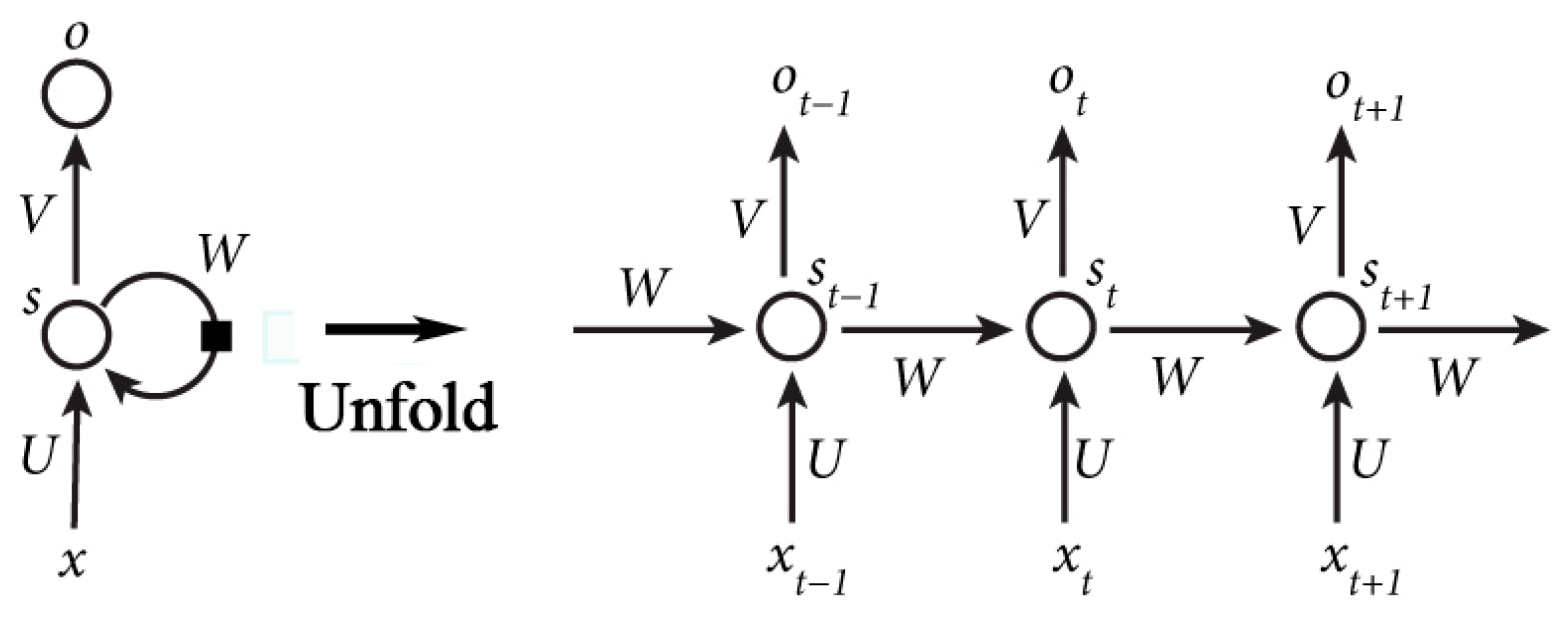
The recurrent neural networks can handle sequential data and have become a hot spot in the fields of machine learning [22,27]. They are networks with loops of several hidden layers that can change monotonously along with the position in a sequence, as shown in Figure 10a. It enables RNN to learn sequential data and Liu [23] has utilized RNN in location prediction with check-in data. Figure 10 shows the structure of RNN. is the vector of the value of the input layer. represents the value of the hidden layer and is the value of the output layer. , are the weight matrix between and , and . is the weight matrix between the value of the hidden layer at time and time .
The RNN can be expressed as Equations (5) and (6), where and are the activation functions. The output of the RNN, namely , is affected by the input . This is the reason why the RNN can take advantage of historical sequential data. Moreover, parameters in the RNN can be further learned with the back propagation through time (BPTT) algorithm [28]. The error term during the weight gradient computing has the property shown in Equation (7), where is the time interval between the current time and historical time. Other parameters is introduced in [29]. When is large (locations that are long time ago), the value of will grows or shrinks very quickly (depending on greater or less than 1). This may cause the learning problems described in [29].
However, location sequences generated by the STS feature extraction could be very long. The RNN may not perform with long sequences. Long short-term memory networks (LSTMs) are a special kind of RNN, capable of learning information for long periods of time [30]. Instead of the simple hidden layer in RNN, LSTM has a more complicated repeating module, as shown in Figure 11. The LSTM uses gates to control the cell states passed from long time ago. The gate is a full connection layer expressed as , where is the weight vector and is the bias. is the sigmoid function so that the output of the gate is 0 to 1.
LSTM utilizes two gates to control the cell state. The forget gate decides how much information of the last cell state will keep to the current time . The other is the input gate, which decides how much information of the input of the current networks will keep to cell state . LSTM uses the output gate to control how much information of the cell state will output to . The expression of the forget gate is shown in Equation (8), where is the weight matrix and is the bias of the forget gate. Similar calculations can be used in the input gate and output gate, as shown in Equations (9) and (12). The cell state of the current input is calculated by the last output and the current input, as shown in Equation (10). As shown in Figure 11, the current cell state is calculated by Equation (11). The output of LSTM , as shown in Equation (13), is decided by and . The training and parameter derivation process can be found in [30]. In conclusion, the conveyor belt-like structure allows LSTM to remove or add information from the very beginning to the current state. Therefore, LSTM is expected to perform well with long sequences.
3.2.2. Model Training and Predicting
The training process. After the STS feature extraction, trajectories are transformed into fixed and discrete sequences with road IDs, expressed as . However, the sequences cannot be directly put into the LSTM model. Each sequence should be divided into segments with fixed length. The length of each segment is determined by specific applications. For example, in the bus system, traces of the past 15 min are used to predict the next location. There are 30 locations collected in 15 min so the length is 30. The length of location segment is defined as . Each location sequence is scanned by a sliding window with fixed width equals to . The window moves forward by one location until it reaches the end of each sequence. Locations in the window are gathered as training features. The next location outside the window is used as label. The process is called feature engineering and is illustrated in Figure 12. Then, each location sequence with features and a label is used to train the LSTM model.
The predicting process. When a new track point is collected, a prediction is not made until all points in a time bin are gathered. Then a representative point is selected from each time bin by the time matching process. Each representative point is mapped to the nearest road in the city road networks. The mapping point is then classified to the nearest fixed road point along the road. The fixed road points are predefined with the distance threshold, which depends on different applications. Each fixed road point has a unique ID. Thus, the new trajectories is transformed into a location sequence represented by road IDs. Then, those IDs are used as the import of the LSTM model for prediction. The predicting process is shown in Figure 13. The model will be re-trained each day during the free time with the trajectories collected in that day to learn the new movement patterns.
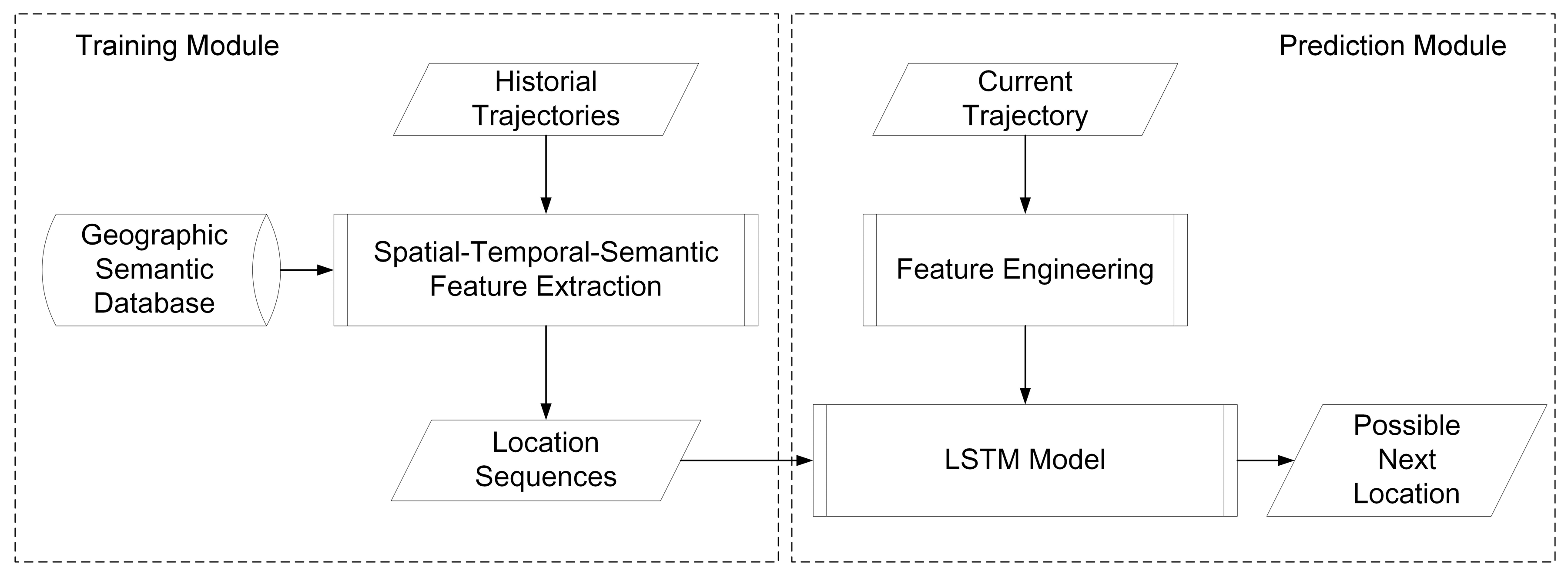
The whole training and predicting processes are shown in Figure 14.
4. Experiments
This section first describes two datasets prepared for evaluation and several evaluation metrics, then introduces several compared algorithms, including a feature selection method and three models. Finally, the experiments are conducted and the results are showed.
4.1. Experimental Preparation
4.1.1. Datasets
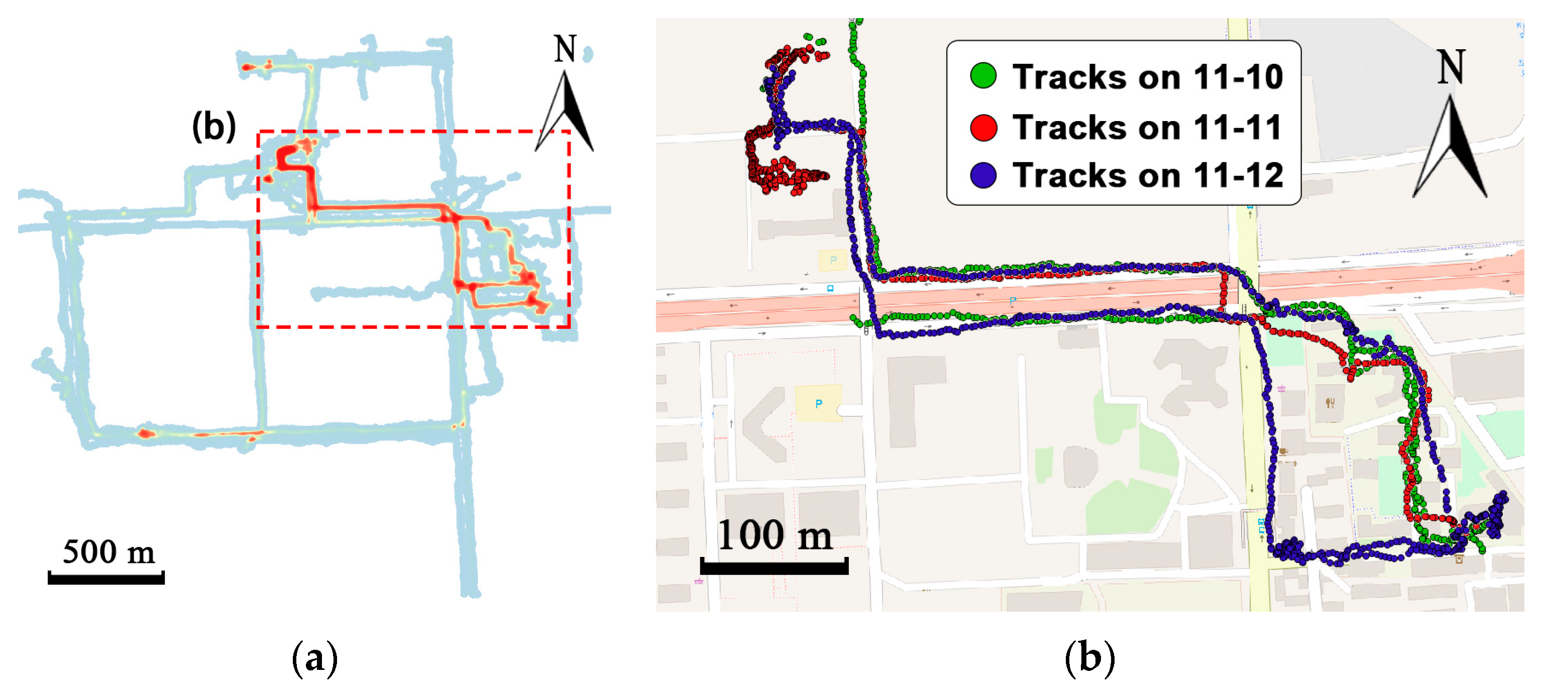
Two real-world trajectory datasets are used to evaluate the proposed method. The courier dataset is a self-collected data from a courier of a food delivery platform in Beijing, China. By installing an application that can collect track points on the courier’s mobile phone, tracks of the courier on 66 working days from 10 November 2016 to 19 January 2017 are recorded. One of the major concerns of the food delivery system is where the courier will go so as to estimate the travel time to the customer. The courier is in charge of a certain area, so there exists a regular route. As shown in Figure 15a, the tracks in the red rectangle have high density, which means the courier always travel along this routes. Figure 15b shows the trajectories of the courier in the red rectangle in three working days.
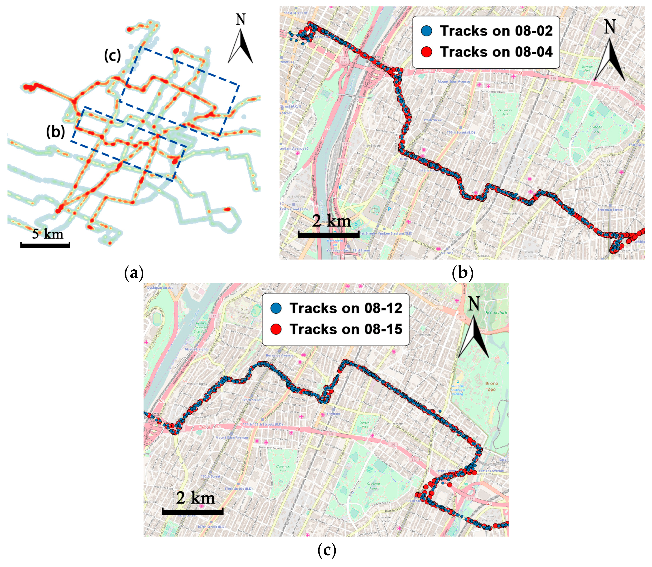
The MTA Bus dataset is provided by the Metropolitan Transportation Authority (MTA) and is available online [31]. The dataset contains trajectories of 5725 buses from 315 bus routes across the New York region, from 1 August to 31 October 2014. The 90-days data contains a very large amount of track points in total, and the average number of points each day is nearly 4.2 million. Trajectories of a bus from route BX36 are selected. As shown in Figure 16a, the red regions in the heat map represent the frequent routes of the bus. There are several frequent routes over a long period of time because the bus may change the route due to rescheduling [29]. However, movements of the bus in each route over a short period of time appear regularly. The trajectories in the blue rectangle in the middle of Figure 16a are frequent, as shown in Figure 16b. Trajectories at the top of Figure 16a are frequent, as shown in Figure 16c.
Table 3 summarizes the characteristics of the two representative datasets. The courier and the MTA bus dataset contain 198 and 149 trajectories respectively, and the time spans are 66 and 90 days. The courier dataset contains 1746 points per day on average and the sampling rate is 0.5 Hz. The sampling rate of the bus dataset is 0.03 Hz, which leads to a smaller number of points per day. The average daily travel distance of the bus is 58 km, far more than the courier. The bus has longer routes than the courier, so the average distance between two points is 23 times more than the courier. Parameters, such as time bin size and distance thresholds, should be set according to the characteristics of the datasets.
4.1.2. Evaluation Metrics
Trajectories are consist of track points that are continuous in space and time. Before to using prediction models, each of the points should be transformed into discrete codes associated to specific regions. This is done so that the learning of models can be done more efficiently and the prediction result can be more precisely. Traditional cell-based methods such as the Geohash convert points into grids. The proposed STS feature extraction utilizes a more accurate way to map each track point to the fixed point on the nearest road. Both methods will cause approximation errors between the original points and the representative points. The average sphere distance between the original points and the representative points is called the deviation distance, as shown in Figure 17. The deviation distance of Geohash is the average distance between each track point and the central point of the grid. The deviation distance of the STS is the average distance between each track point and the fixed point on the nearest road. The deviation distance is used to evaluate the performance of the STS feature extraction method.
In order to measure the performances of different methods, several evaluation metrics are used, including precision, recall, and F-score. The problem of location prediction can be defined as the classification problem. The prediction model predicts the location ID with the highest probability among all location IDs that the object may visit. For classification problems, the samples can be divided into four categories, namely true positives, true negatives, false positives, and false negatives, which are shown in Table 4.
The precision is the fraction of retrieved documents that are relevant to the query. The recall is the fraction of the documents that are relevant to the query that are successfully retrieved, as shown in Equations (14) and (15). For example, if the historical movements of the object shows that there are total of five locations (ID 1 to 5). Four location sequences are going to be predicted and the truth of the next location is (1, 1, 3, 5). The result given by the model is (1, 2, 1, 5). For location 1, , , , . Thus, the precision and recall are 0.5, respectively. Usually, the average precision and recall for all locations are calculated. Moreover, in order to measure the overall performance of the model, F-score is considered, which contains both the precision and the recall, as shown in Equation (16).
4.1.3. Selection of Compared Algorithms
Feature extraction methods. Partitioning trajectories into self-defined cells or grids is commonly used [8,17,18,21]. However, cell-based methods are easily affected by the granularity of the grid and it is difficult to draw a grid in the global area. Geohash is a geocoding system invented by Gustavo Niemeyer [32]. It is a hierarchical spatial data structure that subdivides space into buckets of grid shape and is used as indexing algorithm by many geospatial databases, such as Elasticsearch and MongoDB. For example, a part of trajectory ((−25.383, −49,266), (−25.427, −49.315)) can be transferred to (6gkzwgjz, 6gkzmg1w) by Geohash. Similar to cell-based methods, Geohash extracts the geographic feature of trajectory but may suffer from granularity problems.
Prediction Models. After feature selection, the location sequences are put into different models. Among all of the models described in Table 1, supervised learning models are suitable to fit the location sequences generated by the feature extraction method. The current locations are set to be features and the next location is the label. The location prediction can be regarded as classification problem. The hidden Markov model (HMM) is widely used in location prediction [16,17,18] and gain better prediction results. Moreover, XGBoost [33] is a popular classification and regression model. In many machine learning problems and data science challenges, XGBoost always surpasses other traditional classification models. Recently, the recurrent neural network (RNN) has been employed for mining location sequences [23] and provided a promising future. Therefore, HMM, XGBoost, and RNN are used to compare the proposed method. Brief introductions of HMM and XGBoost are provided below. Details of RNN has been introduced in Section 3.2.1.
The HMM assumes the sequences are generated by a Markov process with unobserved states [34]. Each state has a probability distribution over the possible locations to be visited. It also has a probability distribution over the possible transitions of the states that will be predicted. The probability distribution of the hidden variable at time t depends only on the value of the hidden variable at time t – 1. This is called the Markov property. The prediction task is to compute the probability of a particular output sequence being observed. The probability of observing a particular sequence in the form , where is the location visited at time t, is given by
In Equation (17), the sum runs over all possible hidden-node sequences , where is the hidden state at time at time t. This problem can be solved by the Baum-Welch algorithm. For more information about the derivation of the parameters in HMM, please refer to the tutorial by Rabiner [34].
XGBoost [33] is an ensemble model based on a gradient boosting decision tree (GBDT) [35] and is designed to be highly efficient, flexible, and portable. XGBoost is used for supervised learning problems, where training data with multiple features (current location sequence) are used to predict a target variable (the next location). For tree ensemble learning, the model is defined as Equation (18), where is the number of trees, is a function in the functional space , and is the set of all possible CARTs. The objective function can be written as Equation (19), where the first part is the training loss and the second part is the complexity of the tree, functioning as the regularization. The training method and the parameter derivation process can be found in [33].
4.1.4. Experimental Settings
The evaluation consists of internal comparison and external comparison. The internal comparison focuses on the parameter settings in the STS feature extraction. The external comparison aims to compare the performance with different feature selection methods and model building methods. Table 5 summarizes the experimental settings. Both the courier dataset and the MTA bus dataset are split into a training set (consisting of 90% of the data) and a testing set (10% of the data), respectively. The courier dataset contains 60 days’ data for training, and six days for testing. The MTA bus dataset contains 81 days’ data for training, and nine days for testing. The amount of testing samples meet the demand of real-life applications.
4.2. Evaluation Based on Internal Comparison
In the STS feature extraction, the size of time bin used to allocate track points into time bins and a representative point is selected from each time bin. Then each representative point is mapped to a fixed point on the road by the distance threshold. As mentioned before, these two parameters are determined by the demand of applications. If the trajectories are sampled at a higher rate, smaller time bin sizes and distance thresholds could be selected to achieve more accurate prediction. The sampling time interval of the courier dataset is 2 s, and 30 s of the MTA bus dataset. Therefore, in the courier dataset, the time bin size is set to 4 s, 8 s, and 16 s separately, and the distance threshold is set to 5 m, 10 m, and 15 m. In the bus dataset, time bin size is set to 30 s, 60 s, and 90 s. The average distance of two sampled points is 82.2 m, so the distance threshold of the bus is set to 50 m, 100 m, and 150 m. Then features are imported to the same LSTM model, with fixed . Different prediction precisions are recorded in Table 6 (the courier dataset) and Table 7 (the MTA bus dataset).
4.3. Evaluation Based on External Comparison
In this section, the STS feature extraction method is compared with Geohash, and the LSTM-based model is compared separately with several classic models. First, the Geohash partitioning algorithm is implemented to transform trajectory into cells. The optimal parameter of the Geohash is set to 8, indicating that the side length of a cell is 19 m. The size of time bin and the distance threshold in the courier dataset are set to 16 s and 10 m, which become 30 s and 50 m in the MTA bus dataset. of the location sequence is set to 20 and other parameters of the model are fixed during the comparison. The result is shown in Table 8.
Furthermore, to evaluate the performance of the LSTM model, several classic models are used for comparison. The HMM model is implemented in Python. Optimal parameters are set as follows: the cost used in the forward part of the forward-backward algorithm is set to 0.1, , . The XGBoost method is implemented in Python by the “XGBoost” package. The tuning parameters in XGBoost are numRound, eta, maxDepth, scalePosWeight, minChildWeight, etc. Five-fold cross-validation is used to tune the parameters. Parameter tuning method can be found in [36] in detail. Optimal parameters are set as follows: , , , , .
RNN and LSTM are implemented in Python using the “Keras” package. As introduced in Section 3.2, RNN and LSTM have similar ideas of the hidden loop layer but LSTM is more complicated. There exists similarities in the parameter setting of RNN and LSTM. They both share the activation function as and . To avoid over-fitting, the dropout of each layer is set to 0.2. The categorical cross-entropy is selected as the loss function and the RMSprop algorithm is utilized to update the weights. defines the number of samples that are going to be propagated through the network and is set to 100. is used to train the data. The experiments were executed on a MacOS Sierra platform with a 2.8 GHz i7 CPU and 4 GB RAM.
Evaluation based on performance. The size of time bin and the distance threshold in the courier dataset are set to 16 s and 10 m, which become 30 s and 50 m in the MTA bus dataset. The same location sequences from the STS feature extraction with are used as the input. After tuning the optimal parameters for each model, training data is imported and the results of the prediction of different prediction models are listed in Table 9.
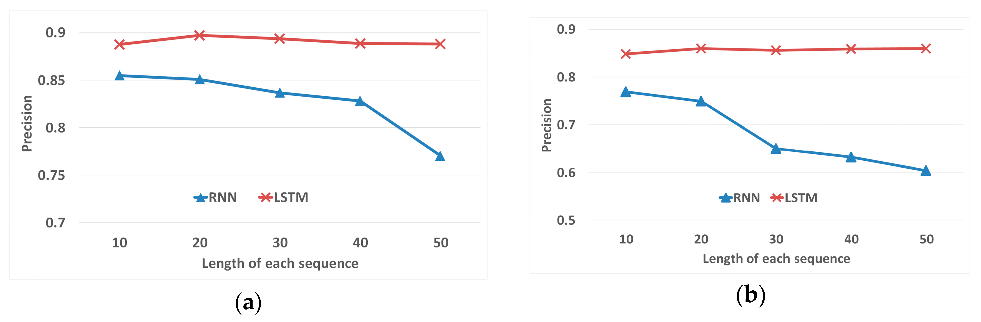
Evaluation based on the length of each sequence. The main difference between RNN and LSTM is the ability to learn long sequences. In the follow experiment, all other parameters and training data are kept the same, except for the . is set from 10 to 50 and the precisions of RNN and LSTM on two datasets are shown in Figure 18. The horizontal axis represents the length of each sequence and the vertical axis is the precision of prediction.
Evaluation based on the size of datasets. Experiments are executed to evaluate the influence of data size on the performance of the LSTM-based model. Two datasets are used and the training data are sampled randomly by 20%, 40%, 60%, 80%, and 100% of the original size. Testing data remains the same. The number of samples are listed in Column 1, and the results are shown in Table 10.
4.4. Evaluation Based on Visualization
The proposed algorithm is designed to solve practical problems in applications such as food delivery or bus system. One basic need of these services is to visualize the result of the predicted location on the map. In this section, the result of the proposed algorithm is drawn by the QGIS software, cooperated with the map data stored in the PostgreSQL. A trajectory from the courier dataset that has never been used in the training is used as test data, showed as the blue line in Figure 15a. During the STS feature extraction, time bin size is set to 2 s, and the distance threshold is the max length of each road for better visualization. Points mapped to the same road will be represented by one road ID and the location is visualized by the road segment. The location sequence after the feature extraction is (391182785, 391187049, 162362370, 163825162, 121991160, 121657041, 122100440,177353870, 22799950, 177353867, 22799950, 177353867), represented by the orange lines with road id in Figure 15a. For better and concise illustration, the location sequences of the fixed road IDs are replaced as (ID0, ID1, ID2, ID3, ID4, ID5, ID6, ID7, ID8, ID9, ID8, ID9).
The of the LSTM model is set to 5. Suppose that the current and latest four locations are collected and used as test data, as shown in Figure 15b. The rest of the sequence is used as the ground truth. The predicted location of (ID0, ID1, ID2, ID3, ID4) given by the LSTM model is ID5. The distance between the actual point and the prediction is calculated by the deviation distance, which is 11.6 meters. Then ID5 is added to the location sequences and a new sequence (ID1, ID2, ID3, ID4, ID5) is imported to the model. The output of the model is 11.5 m away from the actual point. The process is repeated and the results are listed in Table 11. All seven locations in the ground truth are successfully predicted because the deviation distance is relatively small. The seven predicted locations are drawn step by step with different colors in Figure 19c. The LSTM model will continuously predict even though the raw trajectory has ended. The next five locations are shown in Figure 19d.
4.5. Discussion
Performance of the STS feature extraction. During the experiments, internal parameters of the STS feature extraction including the size of time bin and the distance threshold are adjusted to observe the variation of the prediction precision. The results are shown in Table 6 and Table 7. There exists an overall trend that the precision, recall, and F-score of the courier datasets are higher than the bus datasets. From the comparison between the two datasets, as shown in Table 3, the courier data is more precise because the average sampling rate and the average distance between two track points are much less than the bus data. Furthermore, predictions with smaller time bin size are better. With smaller time bin, more locations are extracted from raw trajectories, so the model will learn more and offer better predictions. According to the demand of certain application, the time and distance thresholds of the courier data are set to 16 s, 10 m, and 30 s, 50 m for the bus data.
Results in Table 8 indicate that the STS outperforms Geohash on both datasets. The STS feature extraction method has achieved low deviation distance, which mean that mapping to the nearest points on the road is more precisely than mapping to the central of the Geohash grid. The precision rate of the proposed method is 10.4% higher than Geohash on the courier dataset, and 27.1% higher than that of the bus dataset. Therefore, the STS algorithm has achieved a stable result by mapping trajectory to fixed reference points while keeping the spatial, temporal, and semantic information of the raw trajectory.
Performance of the LSTM-based model. The location sequences generated by the STS feature extraction algorithm are used to train different models. First, parameter tuning methods are utilized to ensure each model is in the best status. Then models are trained by the same location sequences with .
- (1)
- Precision, recall, and F-score. The results showed in Table 9 indicate that the RNN and LSTM outperform the other two classification models on both datasets. Though HMM and XGBoost utilize different ideas of classification, neither of them can take advantage of temporal information. However, neural network-based models are designed for sequential data, which can take advantage of the recent locations as well as the past locations. The precision of RNN is 17.1% higher than the XGBoost and the precision of LSTM is 25.1% higher than the XGBoost. The LSTM achieves the best performance on both datasets. Training time of LSTM is similar to XGBoost and the prediction time is tolerable.
- (2)
- Performance on different lengths of each sequence. Furthermore, experiments have been conducted to evaluate the differences between LSTM and RNN. By alternating the length of the input sequence from 10 to 50, the advantages of LSTM gradually revealed. As illustrated in Figure 18, when the length of location sequence is short, RNN is slightly less than LSTM. However, the performance of RNN declines rapidly when the length is larger than 30. LSTM remains steady on both datasets and performs better than RNN dealing with long sequences.
- (3)
- Performance on different sizes of data. As shown in Table 10, the performance of the LSTM increases as more data is used for training. In the courier dataset, the precision of prediction with 100% of training data is 5.5% higher than training with 20% data. In the MTA bus dataset, the precision of prediction with 100% of training data is 17.3% higher than training with 20% data. The data quantity of the bus dataset has greater impact on the courier dataset. As discussed in Section 4.1.1, the movements of the courier along the same route are more frequent in a short period of time. Therefore, the LSTM can learn the pattern with a small quantity of training data if the data is of good quality. The amount of data used for training depends on specific applications.
- (4)
- Visualization Analysis. The trajectory of the courier is transformed to a sequence of road ID. Though there might be many points on one road, only one road ID is selected as representative for better visualization. All seven predictions are closed to the ground truth. Moreover, the LSTM based model has the ability to generate location sequences. The predicted location of the current is used for the next step prediction. As shown in Figure 19d, the trajectory in red shows the return route from the neighborhood back to the restaurant, which is a regular pattern of the courier. However, the precision of the prediction will decline as more predicted locations are put into the model.
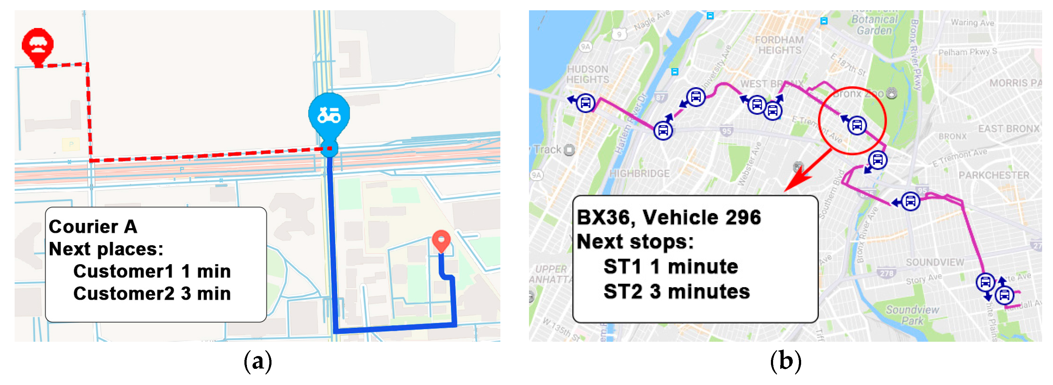
Applications. The proposed STS-LSTM algorithm has advantages on predicting locations on the road, which is suitable for applications such as food delivery and bus system. There are two main application scenarios of the algorithm. The first is the real-time location visualization. For example, in food delivery system, locations of the courier may not be uploaded all the time. It may decline the user’s satisfaction if no positions are showed on the map. The algorithm can predict the location of the courier based on the latest observation, as shown in Figure 20a. The blue point is the predicted location where the courier is right now. Moreover, the result of prediction can be used to estimate the arrival time. For example, location sequences of bus 296 can be generated based on its current location. The time interval of each location is 30 s, and the arrival time to the next stop can be calculated, as shown in Figure 20b.
5. Conclusions
In this paper, a spatial-temporal-semantic neural network algorithm for location prediction is proposed. The algorithm consists of two steps, the spatial-temporal-semantic (STS) feature extraction and the LSTM-based model building. Aiming at solving the problem that traditional methods based on cell partitioning or clustering ignore a large amount of information about points along the road, the STS feature extraction algorithm is proposed. The method transforms the trajectory into location sequences by mapping track points to fixed and discrete points in the road networks. The STS can take advantage of points along the road, which meets the demand of services like delivering systems and transportation systems. After feature extraction, trajectories are transformed into long location sequences. Traditional models cannot perform well with long sequential data; therefore, an LSTM-based model is proposed to overcome the difficulty. The model can better deal with long location sequences to gain better prediction results. Experiments on two real-world datasets show that the proposed STS feature extraction algorithm has lower deviation distance. The location sequences generated by the STS can improve the prediction precision by 27%. Moreover, the proposed LSTM-based model can improve the precision of 25% compared with traditional classification models. The STS-LSTM algorithm has stable and better performance on both datasets.
There are several potential extensions of this paper. Aiming at solving practical problems, the algorithm should be robust to trajectory of poor quality. More data preprocessing works, such as data compression, noise filtering, and data filling could be done in the future. Moreover, the LSTM-based model could be further modified to accept more features and dimensions, such as temporal features like month, week, and day, and semantic features, like stay points. Moreover, LSTM could be combined and intercepted into other classification models, or replaced by a similar but simpler structure called the gated recurrent unit (GRU) [37].
Acknowledgments
This paper is supported by the National Natural Science Foundation of China (No. 41501485).
Author Contributions
Fan Wu and Kun Fu conceived and designed the experiments; Fan Wu and Zhibin Xiao performed the experiments; Fan Wu, Xingyu Fu, and Yang Wang analyzed the data; Fan Wu wrote the paper.
Conflicts of Interest
The authors declare no conflict of interest.
References
- Koren, Y.; Bell, R.; Volinsky, C. Matrix factorization techniques for recommender systems. Computer 2009, 42, 30–37. [Google Scholar] [CrossRef]
- Xiong, L.; Chen, X.; Huang, T.K.; Schneider, J.G.; Carbonell, J.G. Temporal collaborative filtering with bayesian probabilistic tensor factorization. In Proceedings of the Siam International Conference on Data Mining (SDM 2010), Columbus, OH, USA, 29 April–1 May 2010; pp. 211–222. [Google Scholar]
- Zheng, V.W.; Zheng, Y.; Xie, X.; Yang, Q. Collaborative location and activity recommendations with gps history data. In Proceedings of the International Conference on World Wide Web (WWW 2010), Raleigh, NC, USA, 26–30 April 2010; pp. 1029–1038. [Google Scholar]
- Bahadori, M.T.; Yu, R.; Liu, Y. Fast multivariate spatio-temporal analysis via low rank tensor learning. Adv. Neural Inf. Process. Syst. 2014, 4, 3491–3499. [Google Scholar]
- Zhuang, J.; Mei, T.; Hoi, S.C.H.; Xu, Y.Q.; Li, S. When recommendation meets mobile:Contextual and personalized recommendation on the go. In Proceedings of the Ubiquitous Computing, International Conference (UBICOMP 2011), Beijing, China, 17–21 September 2011; pp. 153–162. [Google Scholar]
- Monreale, A.; Pinelli, F.; Trasarti, R.; Giannotti, F. Wherenext: A location predictor on trajectory pattern mining. In Proceedings of the ACM SIGKDD International Conference on Knowledge Discovery and Data Mining, Paris, France, 28 June–1 July 2009; pp. 637–646. [Google Scholar]
- Jiang, B.; Yin, J.; Zhao, S. Characterizing the human mobility pattern in a large street network. Phys. Rev. E Stat. Nonlinear Soft Matter Phys. 2009, 80, 1711–1715. [Google Scholar] [CrossRef] [PubMed]
- Jeung, H.; Liu, Q.; Shen, H.T.; Zhou, X. A hybrid prediction model for moving objects. In Proceedings of the IEEE 24th International Conference on Data Engineering (ICDE 2008), Cancun, Mexico, 7–12 April 2008; pp. 70–79. [Google Scholar]
- Yavaş, G.; Katsaros, D.; Ulusoy, Ö.; Manolopoulos, Y. A data mining approach for location prediction in mobile environments. Data Knowl. Eng. 2005, 54, 121–146. [Google Scholar] [CrossRef]
- Morzy, M. Mining frequent trajectories of moving objects for location prediction. In Proceedings of the International Conference on Machine Learning and Data Mining in Pattern Recognition (MLDM 2007), Leipzig, Germany, 18–20 July 2007; pp. 667–680. [Google Scholar]
- Giannotti, F.; Nanni, M.; Pedreschi, D. Efficient mining of temporally annotated sequences. In Proceedings of the Siam International Conference on Data Mining, Bethesda, MD, USA, 20–22 April 2006; pp. 346–357. [Google Scholar]
- Li, Z.; Ding, B.; Han, J.; Kays, R.; Nye, P. Mining periodic behaviors for moving objects. In Proceedings of the 16th ACM SIGKDD International Conference on Knowledge Discovery and Data Mining, Washington, DC, USA, 25–28 July 2010; pp. 1099–1108. [Google Scholar]
- Li, Z.; Han, J.; Ji, M.; Tang, L.A.; Yu, Y.; Ding, B.; Lee, J.G.; Kays, R. Movemine: Mining moving object data for discovery of animal movement patterns. ACM Trans. Intell. Syst. Technol. 2011, 2, 37. [Google Scholar] [CrossRef]
- Lathia, N.; Hailes, S.; Capra, L. Temporal collaborative filtering with adaptive neighbourhoods. In Proceedings of the International ACM SIGIR Conference on Research and Development in Information Retrieval (SIGIR 2009), Boston, MA, USA, 19–23 July 2009; pp. 796–797. [Google Scholar]
- Cheng, C.; Yang, H.; King, I.; Lyu, M.R. Fused matrix factorization with geographical and social influence in location-based social networks. In Proceedings of the AAAI Conference on Artificial Intelligence, Toronto, ON, Canada, 22–26 July 2012. [Google Scholar]
- Rendle, S.; Freudenthaler, C.; Schmidt-Thieme, L. Factorizing personalized markov chains for next-basket recommendation. In Proceedings of the International Conference on World Wide Web, Raleigh, CA, USA, 26–30 April 2010; pp. 811–820. [Google Scholar]
- Mathew, W.; Raposo, R.; Martins, B. Predicting future locations with hidden markov models. In Proceedings of the ACM Conference on Ubiquitous Computing, Pittsburgh, PA, USA, 5–8 September 2012; pp. 911–918. [Google Scholar]
- Jeung, H.; Shen, H.T.; Zhou, X. Mining Trajectory Patterns Using Hidden Markov Models; Springer: Berlin/Heidelberg, Germany, 2007; pp. 470–480. [Google Scholar]
- Alvares, L.O.; Bogorny, V.; Kuijpers, B. Towards Semantic Trajectory Knowledge Discovery; Springer: Berlin/Heidelberg, Germany, 2007. [Google Scholar]
- Bogorny, V.; Kuijpers, B.; Alvares, L.O. ST-MQL: A semantic trajectory data mining query language. Int. J. Geogr. Inf. Sci. 2009, 23, 1245–1276. [Google Scholar] [CrossRef]
- Ying, J.C.; Lee, W.C.; Tseng, V.S. Mining geographic-temporal-semantic patterns in trajectories for location prediction. ACM Trans. Intell. Syst. Technol. 2013, 5, 2. [Google Scholar] [CrossRef]
- Liu, Q.; Wu, S.; Wang, L.; Tan, T. Predicting the next location: A recurrent model with spatial and temporal contexts. In Proceedings of the Thirtieth AAAI Conference on Artificial Intelligence, Phoenix, AZ, USA, 12–17 February 2016; pp. 194–200. [Google Scholar]
- Mikolov, T.; Karafiát, M.; Burget, L.; Cernocký, J.; Khudanpur, S. Recurrent neural network based language model. In Proceedings of the Conference of the International Speech Communication Association (INTERSPEECH 2010), Makuhari, Chiba, Japan, 26–30 September 2010; pp. 1045–1048. [Google Scholar]
- The Open Street Map Project. Available online: http://www.openstreetmap.org (accessed on 13 February 2017).
- Newson, P.; Krumm, J. Hidden markov map matching through noise and sparseness. In Proceedings of the ACM Sigspatial International Symposium on Advances in Geographic Information Systems (ACM-GIS 2009), Seattle, WA, USA, 4–6 November 2009; pp. 336–343. [Google Scholar]
- Goh, C.Y.; Dauwels, J.; Mitrovic, N.; Asif, M.T. Online map-matching based on hidden markov model for real-time traffic sensing applications. In Proceedings of the 2012 15th International IEEE Conference on Intelligent Transportation Systems (ITSC), Anchorage, AK, USA, 16–19 September 2012; pp. 776–781. [Google Scholar]
- Graves, A.; Mohamed, A.R.; Hinton, G. Speech recognition with deep recurrent neural networks. In Proceedings of the IEEE International Conference on Acoustics, Speech and Signal Processing, Vancouver, BC, Canada, 26–31May 2013; pp. 6645–6649. [Google Scholar]
- Rumelhart, D.E.; Hinton, G.E.; Williams, R.J. Learning representations by back-propagating errors. Cogn. Model. 1988, 5, 1. [Google Scholar] [CrossRef]
- Bengio, Y.; Simard, P.; Frasconi, P. Learning long-term dependencies with gradient descent is difficult. IEEE Trans. Neural Netw. 1994, 5, 157. [Google Scholar] [CrossRef] [PubMed]
- Hochreiter, S.; Schmidhuber, J. Long short-term memory. Neural Comput. 1997, 9, 1735–1780. [Google Scholar] [CrossRef] [PubMed]
- The MTA Bus Dataset. Available online: http://web.mta.info/developers/MTA-Bus-Time-historical-data.html (accessed on 13 February 2017).
- The Geohash Algorithm. Available online: https://en.wikipedia.org/wiki/Geohash (accessed on 13 February 2017).
- Chen, T.; Guestrin, C. Xgboost: A scalable tree boosting system. In Proceedings of the 22nd ACM SIGKDD International Conference on Knowledge Discovery and Data Mining, San Francisco, CA, USA, 13–17 August 2016; pp. 785–794. [Google Scholar]
- Rabiner, L.R. A tutorial on hidden markov models and selected applications in speech recognition. Read. Speech Recognit. 1990, 77, 267–296. [Google Scholar]
- Friedman, J.H. Greedy function approximation: A gradient boosting machine. Ann. Stat. 2001, 1189–1232. [Google Scholar] [CrossRef]
- Complete Guide to Parameter Tuning in Xgboost (with Codes in Python). Available online: https://www.analyticsvidhya.com/blog/2016/03/complete-guide-parameter-tuning-xgboost-with-codes-python/ (accessed on 13 February 2017).
- Cho, K.; Merrienboer, B.V.; Gulcehre, C.; Bahdanau, D.; Bougares, F.; Schwenk, H.; Bengio, Y. Learning phrase representations using rnn encoder-decoder for statistical machine translation. Comput. Sci. 2014. [Google Scholar]
Figure 1.
Trajectories of a courier during continuous working day from Hangzhou, China, which appeal regularity. (a) Track on 12 August 2016; (b) Track on 13 August 2016; (c) Track on 14 August 2016.
Figure 1.
Trajectories of a courier during continuous working day from Hangzhou, China, which appeal regularity. (a) Track on 12 August 2016; (b) Track on 13 August 2016; (c) Track on 14 August 2016.

Figure 2.
The frequent patterns of the courier.

Figure 3.
The accuracy of the prediction is influenced by the granularity of the cell partition. Track points from a courier in Hangzhou, China. (a) Partitioning into large cells and smaller cells; (b) The actual boundaries of the neighborhoods.
Figure 3.
The accuracy of the prediction is influenced by the granularity of the cell partition. Track points from a courier in Hangzhou, China. (a) Partitioning into large cells and smaller cells; (b) The actual boundaries of the neighborhoods.
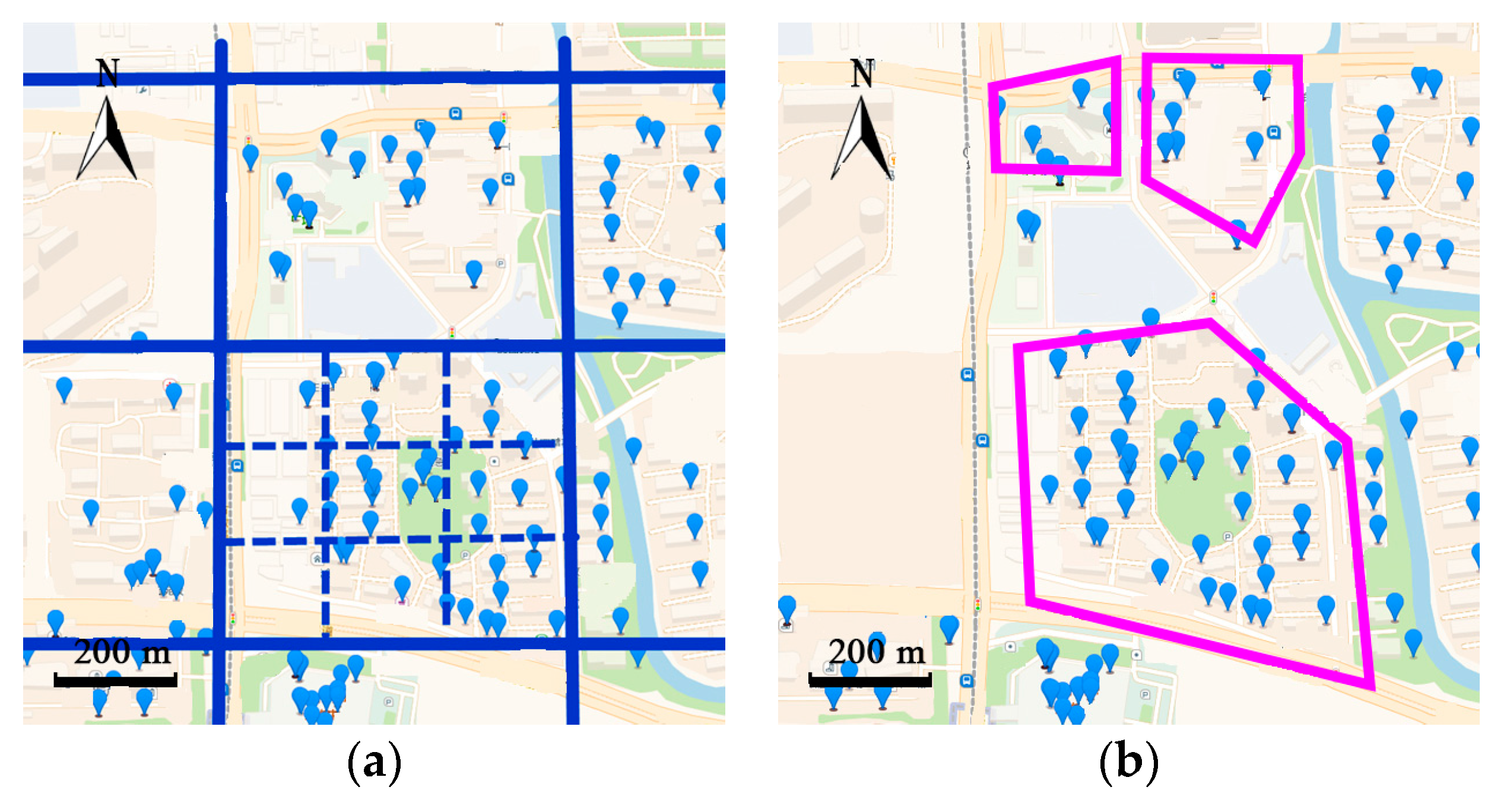
Figure 4.
The necessity of transforming trajectories into discrete and fixed locations.

Figure 5.
Flowchart of the STS-LSTM.

Figure 6.
Process of the mapping of time bins.
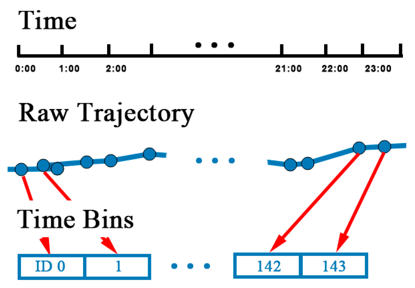
Figure 7.
The road network data of Beijing, used as reference points in the geo-feature mapping.
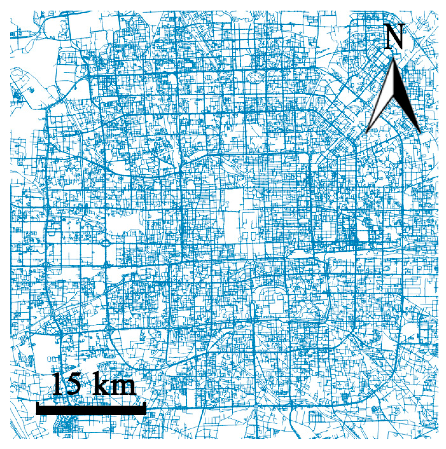
Figure 8.
Process of the geographic feature mapping. (a) Projection of each track point to the nearest line; (b) calculated fixed points on the line by ; (c) mapping track points to the nearest fixed points.
Figure 8.
Process of the geographic feature mapping. (a) Projection of each track point to the nearest line; (b) calculated fixed points on the line by ; (c) mapping track points to the nearest fixed points.

Figure 9.
A running example of the spatial-temporal-semantic feature extraction. (a) The blue dots are the original trajectory. The red dots is the track points after temporal matching. (b) The red dots are the location sequences after the geographical and semantic feature matching.
Figure 9.
A running example of the spatial-temporal-semantic feature extraction. (a) The blue dots are the original trajectory. The red dots is the track points after temporal matching. (b) The red dots are the location sequences after the geographical and semantic feature matching.
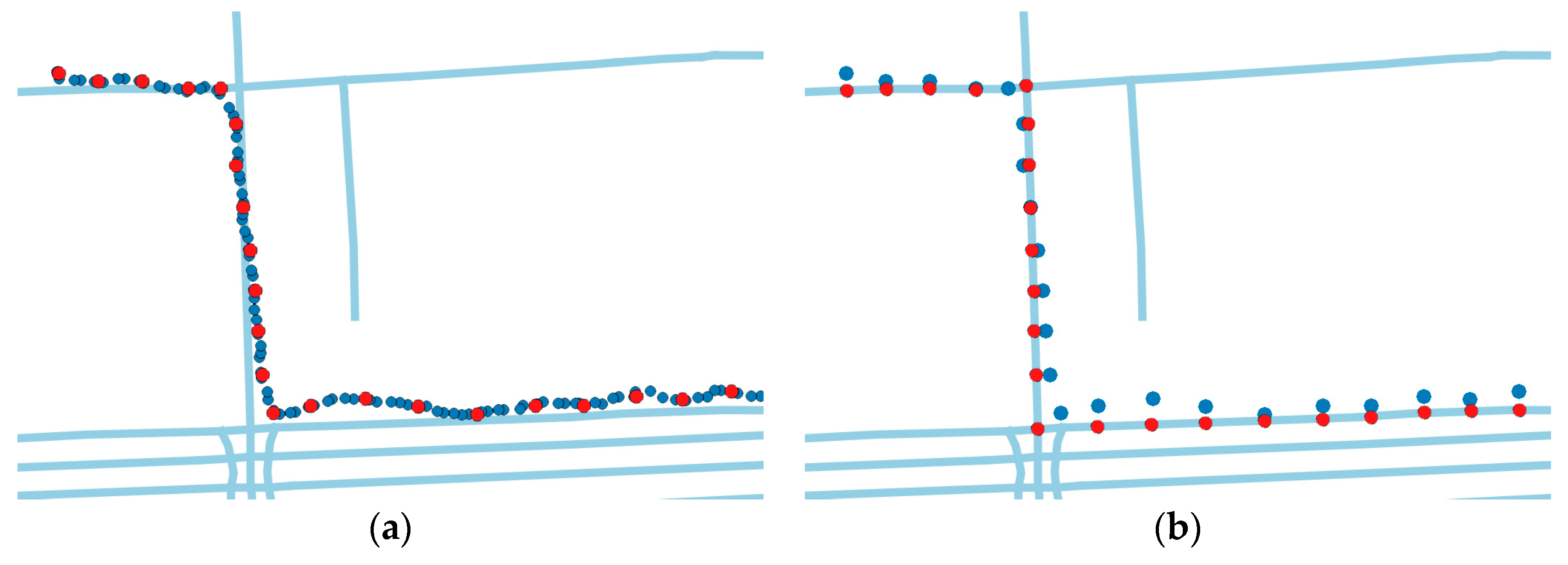
Figure 10.
The structure of the RNN.

Figure 11.
The structure of the repeating module in the LSTM.
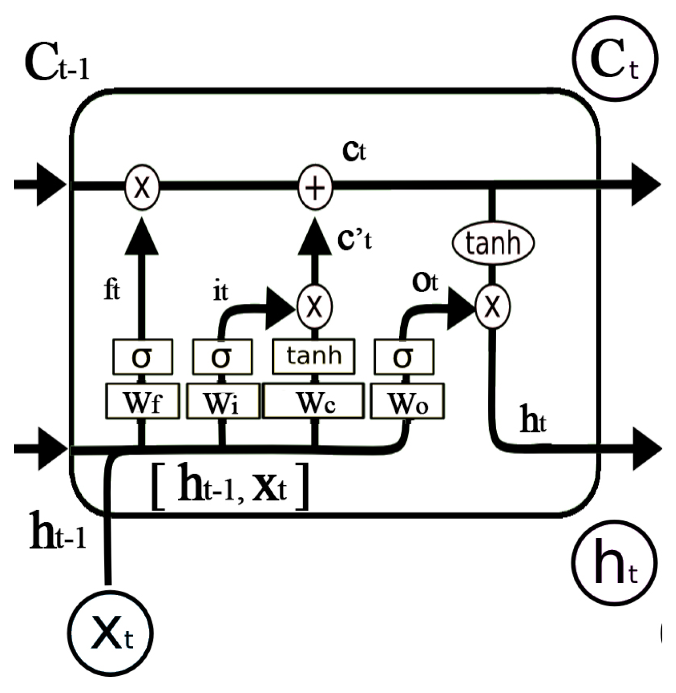
Figure 12.
The process of feature engineering.
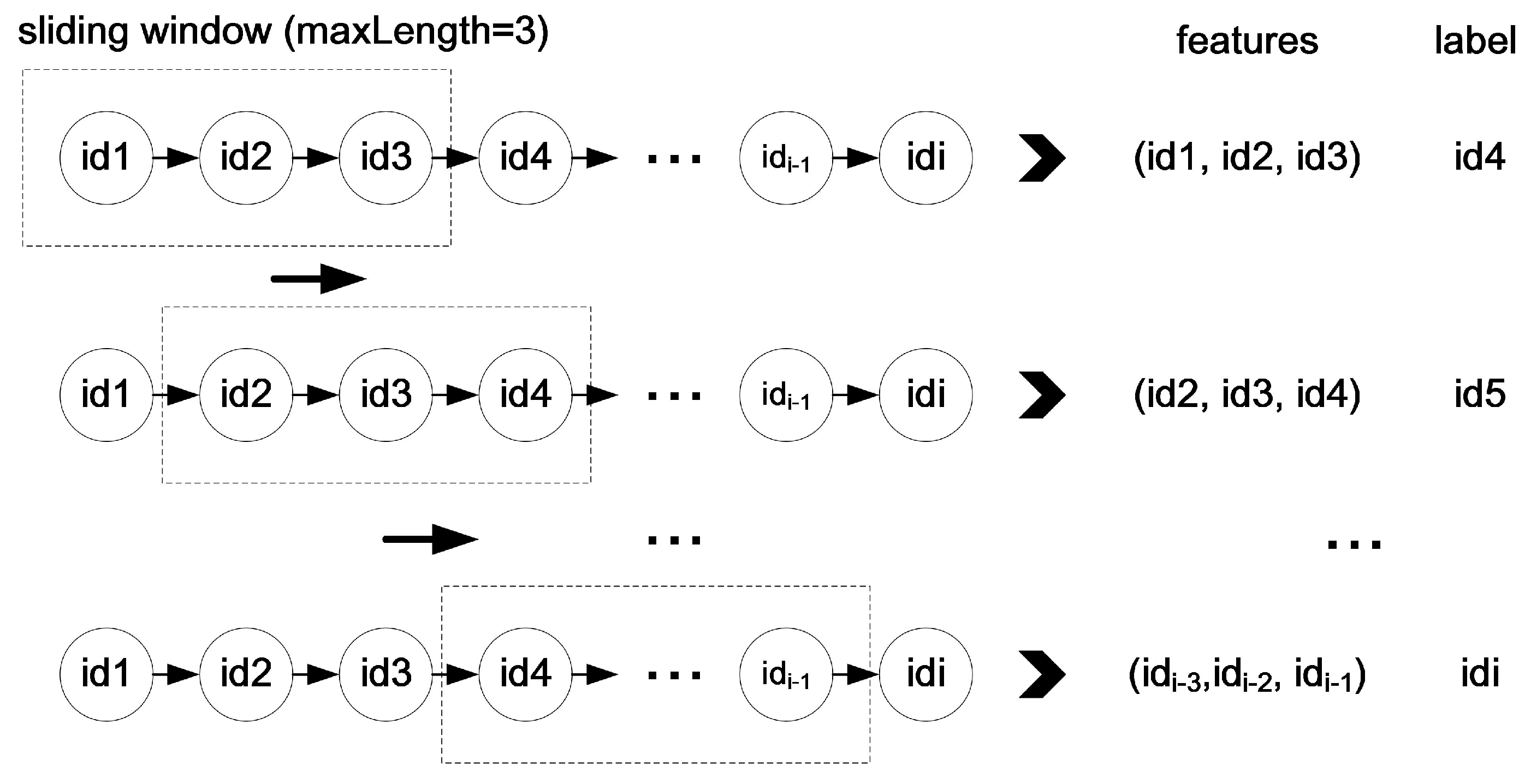
Figure 13.
The process of feature engineering.
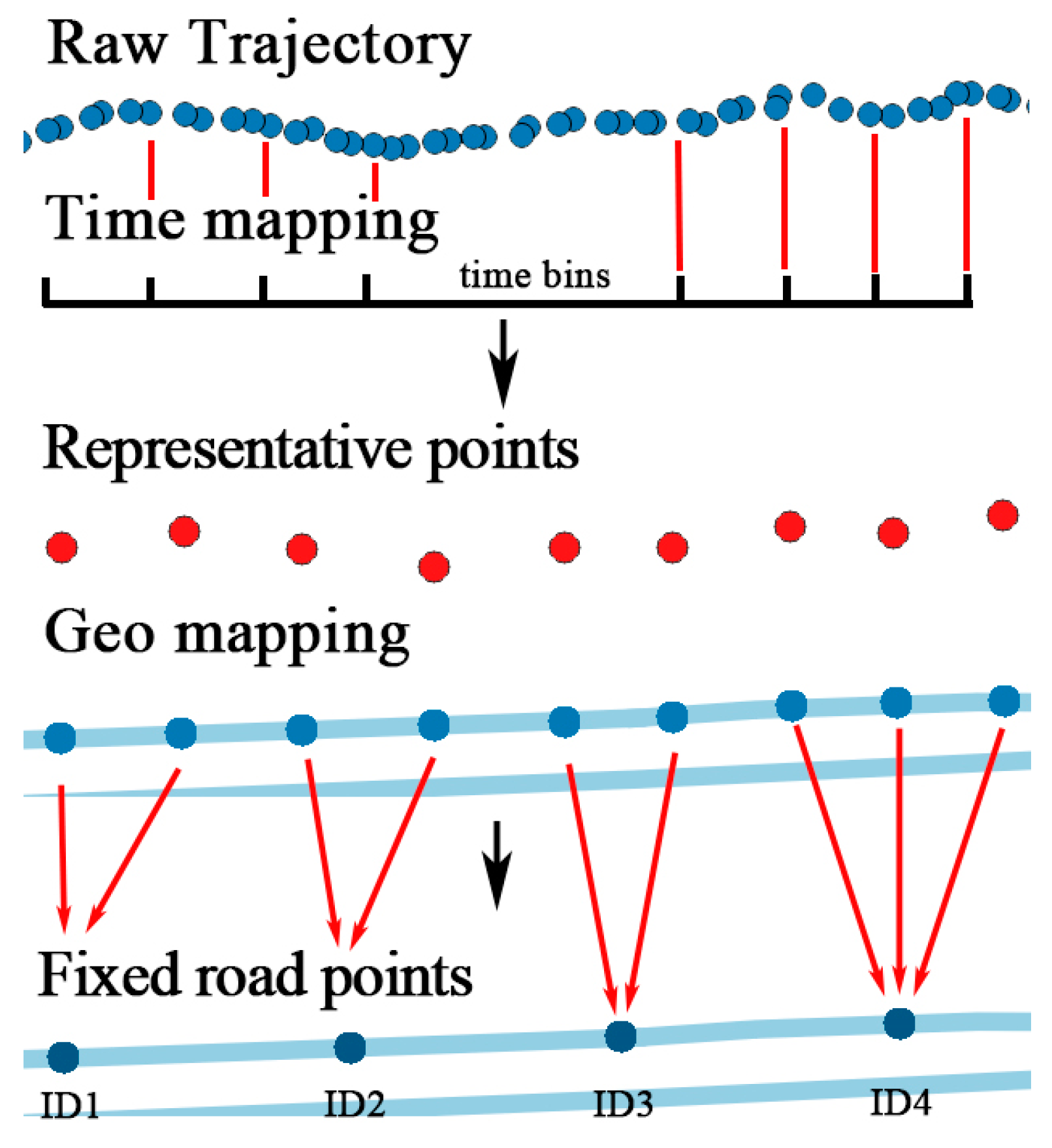
Figure 14.
The processes of the model training and location predicting.

Figure 15.
Visualization of the trajectories of a courier from the courier dataset. (a) The heat map of all the tracks in the courier dataset. (b) Trajectories from 10 November to 12 November.
Figure 15.
Visualization of the trajectories of a courier from the courier dataset. (a) The heat map of all the tracks in the courier dataset. (b) Trajectories from 10 November to 12 November.

Figure 16.
Visualization of the MTA bus dataset. Trajectories of bus whose ID is 296 are selected. (a) The heat map of all the tracks in the MTA bus dataset. (b) Trajectories on 2 and 4 August. (c) Trajectories on 12 and 15 August.
Figure 16.
Visualization of the MTA bus dataset. Trajectories of bus whose ID is 296 are selected. (a) The heat map of all the tracks in the MTA bus dataset. (b) Trajectories on 2 and 4 August. (c) Trajectories on 12 and 15 August.

Figure 17.
The calculation of deviation distance. (a) The deviation distance of the Geohash. (b) The deviation distance of the STS feature extraction.
Figure 17.
The calculation of deviation distance. (a) The deviation distance of the Geohash. (b) The deviation distance of the STS feature extraction.
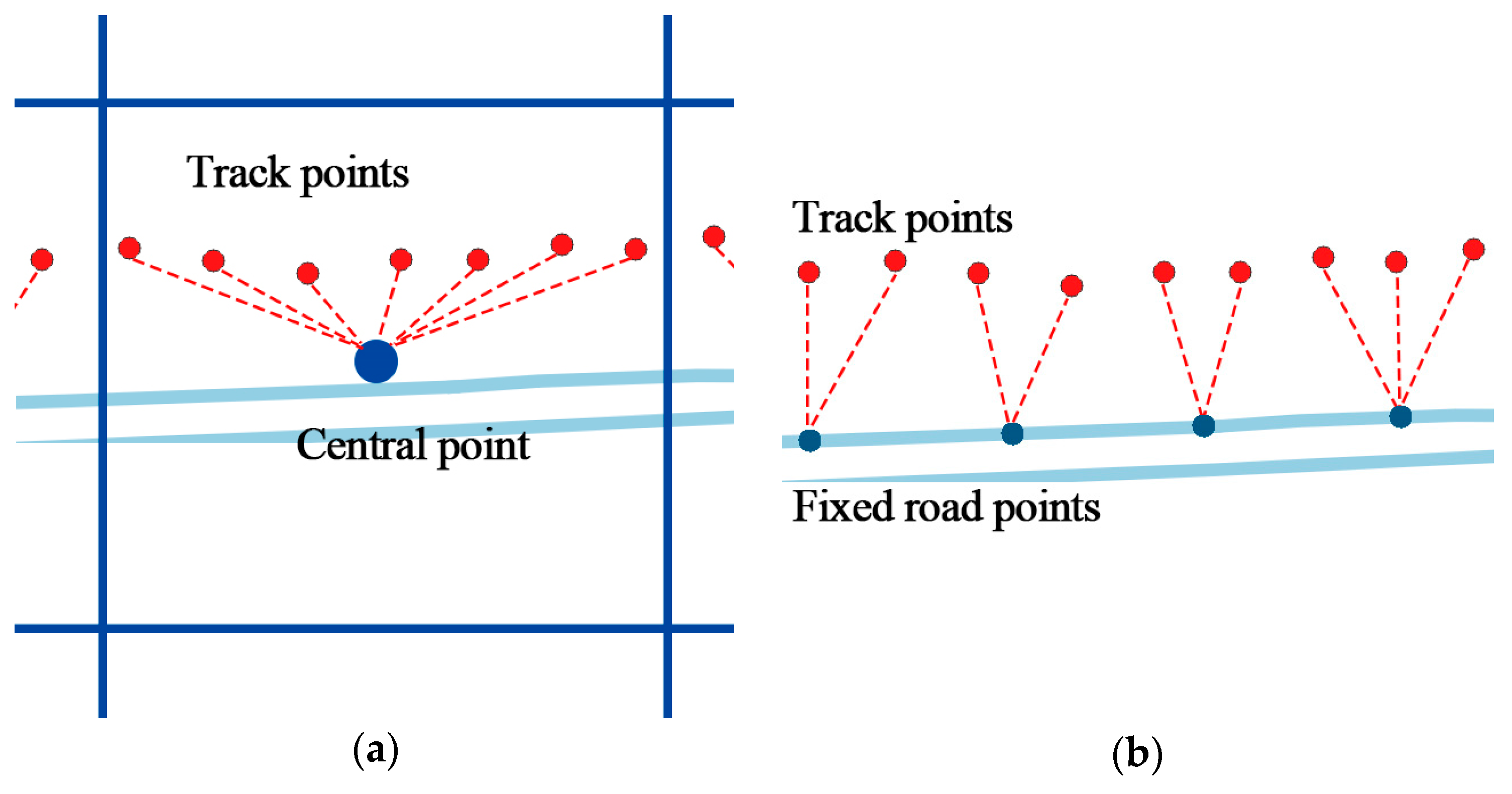
Figure 18.
Figure of the comparison between RNN and LSTM of the ability to handle long sequences. (a) Results on the courier dataset; (b) Results on the MTA bus dataset.
Figure 18.
Figure of the comparison between RNN and LSTM of the ability to handle long sequences. (a) Results on the courier dataset; (b) Results on the MTA bus dataset.

Figure 19.
Visualization of the prediction results. (a) Blue line represents the raw trajectory, and the orange line is the location sequence after STS feature extraction. (b) Current locations of the courier. (c) The next five predicted locations by the algorithm in five iterations, marked as different colors. (d) Further predictions that exceed the original trajectory.
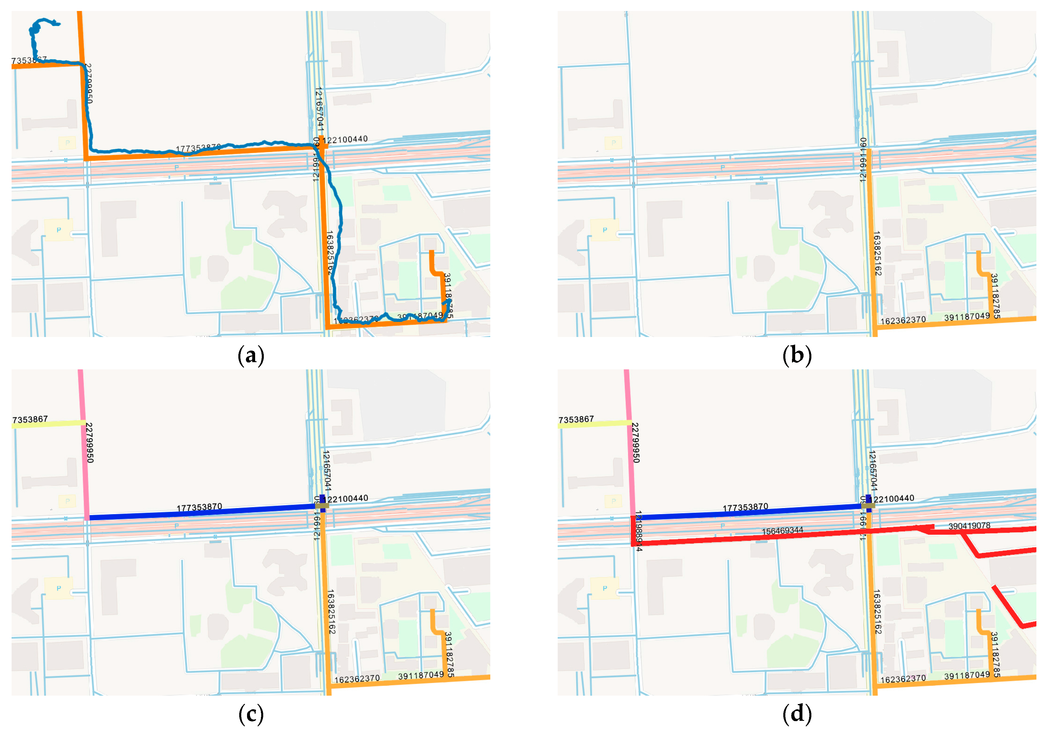
Figure 20.
Application scenarios of the STS-LSTM algorithms. (a) In a food delivery system, given the last location (the red circle) and the current location (the blue point), the next location can be predicted (the red point on the left). (b) In a bus system, the location predicted can be used to estimate the arrival time of each bus stop.

Table 1.
Summary of location prediction methods.
| Methods | Studies | Data Type | Model Type | Specialties | |
|---|---|---|---|---|---|
| Location Recommender | Koren [1] | Event data | Recommender/Simple models | Matrix Factorization | |
| Xiong [2] | Event data | Tensor Factorization | |||
| Zheng [3] | Trajectory | Spatial Factorization | |||
| Bahadori [4] | Check-in data | Spatial-temporal Tensor Factorization | |||
| Zhuang [5] | Event data | Geo-location, time | |||
| Monereale [6] | Trajectory | Using crowds to infer personal behavior | |||
| Movement Pattern Mining | Mobile patterns | Jiang [7] | Trajectory | Simple model | Location sequence, flight pattern |
| Jeung [8], Yavas [9] | Trajectory | Pattern recognition/Unsupervised learning | Motion functions, a priori algorithm | ||
| Morzy [10] | Sensor data | PrefixSpan | |||
| Spatial-temporal patterns | Giannotti [11] | Synthetic sequence | Travel time-aware | ||
| Li [12,13] | Trajectory | Period and swarm pattern | |||
| Prediction Model Building | Neighborhood-based model | Lathia [14] | Event data | Unsupervised learning | Time-aware neighborhood |
| Cheng [15] | LSBNs data | Multi-center Gaussian | |||
| Markov Chain model (MC) | Rendle [16] | Purchase data | Classification/Supervised learning | Factorization Markov Chain | |
| Mathew [17] | Trajectory | Trajectory clustering, Hidden Markov model | |||
| Jeung [18] | Trajectory | Cell partition, Hidden Markov model | |||
| Semantic-based model | Alvares [19] | Trajectory | Pattern recognition/Unsupervised learning | Stop dectection, sequential mining | |
| Bogorny [20] | Trajectory | Hierarchical cluster with semantic | |||
| Ying [21] | Trajectory | Spatial-temporal-semantic, pattern tree | |||
| Neural Network-based model | Liu [22] | Check-in data | Classification/Neural Networks | Spatial-temporal RNN | |
Table 2.
Semantic tags of the road networks.
| Tag (ID) | Name | Type | ... | Coordinates |
|---|---|---|---|---|
| 391182785 | Zhong Guancun East Rd. | Motor | ... | [116.330, 39.982], [116.330, 39.983], ... |
| 391182778 | Bao Fusi Rd. | Bike | ... | [116.329, 39.983], [116.328, 39.983], ... |
Table 3.
Statistics of two trajectory datasets.
| Dataset | Days | Trajs | AvgPts/tra | AvgPts/day | AvgRate (Hz) | AvgDis/pt (m) | AvgDis/day (km) |
|---|---|---|---|---|---|---|---|
| Courier | 66 | 198 | 582 | 1746 | 0.5 | 3.5 | 6.1 |
| MTAbus | 90 | 149 | 710 | 1176 | 0.03 | 82.3 | 58.4 |
Table 4.
Four categories of classification problems.
| True Condition | Predicted Condition | |
|---|---|---|
| Positive | Negative | |
| Positive | True Positives (TP) | True Negatives (FN) |
| Negative | False Positives (FP) | False Negatives (TN) |
Table 5.
Summary of experimental settings.
| Feature Extraction | Model Building | |||||
|---|---|---|---|---|---|---|
| Internal Comparison | STS * | Parameter setting | mLSTM * | |||
| Time bin size | 8/30 s | 16/60 s | 32/90 s | |||
| Distance Threshold | 5/50 m | 10/100 m | 15/150 m | |||
| External Comparison | STS with fixed parameters vs. Geohash | mLSTM | ||||
| STS with fixed parameters | LSTM vs. XGBoost, HMM, RNN | |||||
* STS and LSTM are proposed methods in this paper.
Table 6.
The evaluation results of prediction with different parameter settings of the courier dataset.
Table 6.
The evaluation results of prediction with different parameter settings of the courier dataset.
| Parameter | Precision | Recall | F-Score | |
|---|---|---|---|---|
| Time Bin Size | Distance Threshold | |||
| 8 s | 5 m | 0.9150 | 0.9169 | 0.9130 |
| 10 m | 0.9277 | 0.9252 | 0.9228 | |
| 15 m | 0.9286 | 0.9306 | 0.9267 | |
| 16 s | 5 m | 0.8863 | 0.8803 | 0.8785 |
| 10 m | 0.8975 | 0.8890 | 0.8874 | |
| 15 m | 0.8945 | 0.8863 | 0.8855 | |
| 32 s | 5 m | 0.8474 | 0.8396 | 0.8369 |
| 10 m | 0.8612 | 0.8611 | 0.8564 | |
| 15 m | 0.8704 | 0.8688 | 0.8666 | |
Table 7.
The results of prediction with different parameter settings of the MTA bus dataset.
| Parameter | Precision | Recall | F-Score | |
|---|---|---|---|---|
| Time Bin Size | Distance Threshold | |||
| 30 s | 50 m | 0.8605 | 0.8571 | 0.8511 |
| 100 m | 0.8656 | 0.8633 | 0.8603 | |
| 150 m | 0.8742 | 0.8688 | 0.8652 | |
| 60 s | 50 m | 0.8295 | 0.8204 | 0.8187 |
| 100 m | 0.8369 | 0.8257 | 0.8235 | |
| 150 m | 0.8434 | 0.8324 | 0.8302 | |
| 90 s | 50 m | 0.8118 | 0.8021 | 0.7965 |
| 100 m | 0.8220 | 0.8117 | 0.8068 | |
| 150 m | 0.8301 | 0.8189 | 0.8114 | |
Table 8.
The precision of prediction between Geohash and STS feature extraction on two datasets.
| Datasets | Methods | Avg Deviation Distance (Meters) | Precision | Recall | F-Score |
|---|---|---|---|---|---|
| Courier | Geohash | 53.09 | 0.8377 | 0.8256 | 0.8234 |
| STS Feature | 9.51 | 0.8957 | 0.8890 | 0.8874 | |
| MTA Bus | Geohash | 53.12 | 0.6734 | 0.6648 | 0.6650 |
| STS Feature | 3.35 | 0.8605 | 0.8571 | 0.8511 |
Table 9.
The performance of different models on two datasets.
| Datasets | Methods | Precision | Recall | F-Score | Training Time (s) | Predicting Time (s) |
|---|---|---|---|---|---|---|
| Courier | HMM | 0.6741 | 0.6678 | 0.6709 | 2433.40 | 12.85 |
| XGBoost | 0.7152 | 0.7113 | 0.6897 | 221.33 | 0.33 | |
| RNN | 0.8370 | 0.8462 | 0.8380 | 61.03 | 0.59 | |
| LSTM | 0.8975 | 0.8890 | 0.8874 | 205.73 | 1.43 | |
| MTA Bus | HMM | 0.5378 | 0.5204 | 0.5289 | 4320.42 | 20.67 |
| XGBoost | 0.6012 | 0.5996 | 0.6004 | 450.85 | 1.07 | |
| RNN | 0.7501 | 0.7539 | 0.7520 | 135.67 | 1.21 | |
| LSTM | 0.8605 | 0.8571 | 0.8511 | 654.92 | 4.29 |
Table 10.
The influence of data quantity on the performance of the LSTM models on two datasets.
| Datasets | Data Quantity (Number of Samples) | Precision | Recall | F-Score | Training Time (s) | Predicting Time (s) | |
|---|---|---|---|---|---|---|---|
| Courier | 20% | 2187 | 0.8505 | 0.8528 | 0.8468 | 46.38 | 1.29 |
| 40% | 4375 | 0.8834 | 0.8791 | 0.8749 | 78.89 | 1.33 | |
| 60% | 6563 | 0.8844 | 0.8824 | 0.8794 | 112.04 | 1.44 | |
| 80% | 8751 | 0.8830 | 0.8750 | 0.8722 | 144.51 | 1.36 | |
| 100% | 10939 | 0.8975 | 0.8890 | 0.8874 | 205.73 | 1.43 | |
| MTA Bus | 20% | 8996 | 0.7331 | 0.7381 | 0.7191 | 146.13 | 3.70 |
| 40% | 17992 | 0.8199 | 0.8171 | 0.8067 | 276.48 | 3.73 | |
| 60% | 26989 | 0.8455 | 0.8417 | 0.8338 | 404.66 | 3.85 | |
| 80% | 35985 | 0.8540 | 0.8521 | 0.8430 | 532.62 | 3.98 | |
| 100% | 44982 | 0.8605 | 0.8571 | 0.8511 | 654.92 | 4.29 | |
Table 11.
Running example of the input and output of the prediction model.
| Round | Input Sequence | Predict Location | Ground Truth | Deviation Distance (m) |
|---|---|---|---|---|
| 1 | ID0, ID1, ID2, ID3, ID4 | ID5 (116.327, 39.982) | (116.327, 39.984) | 11.6 |
| 2 | ID1, ID2, ID3, ID4, ID5 | ID6 (116.326, 39.984) | (116.327, 39.984) | 11.5 |
| 3 | ID2, ID3, ID4, ID5, ID6 | ID7 (116.324, 39.984) | (116.324, 39.984) | 16.4 |
| 4 | ID3, ID4, ID5, ID6, ID7 | ID8 (116.321, 39.985) | (116.321, 39.985) | 12.1 |
| 5 | ID4, ID5, ID6, ID7, ID8 | ID9 (116.319, 39.986) | (116.320, 39.987) | 68.6 |
| 6 | ID5, ID6, ID7, ID8, ID9 | ID8 (116.321, 39.985) | (116.321, 39.985) | 30.1 |
| 7 | ID6, ID7, ID8, ID9, ID8 | ID9 (116.319, 39.986) | (116.320, 39.987) | 15.6 |
| 8 | ID6, ID7, ID8, ID9, ID8, ID9 | ID8 | X | X |
| 9 | ID7, ID8, ID9, ID8, ID9, ID8 | 121988914 | X | X |
| 10 | ID8, ID9, ID8, ID9, ID8, 121988914 | 156469344 | X | X |
| 11 | ID9, ID8, ID9, ID8, 121988914, 156469344 | 390419078 | X | X |
| 12 | ID8, ID9, ID8, 156469344, 390419078 | 367394051 | X | X |
| 13 | ... | ... | ... |
© 2017 by the authors. Licensee MDPI, Basel, Switzerland. This article is an open access article distributed under the terms and conditions of the Creative Commons Attribution (CC BY) license (http://creativecommons.org/licenses/by/4.0/).
Share and Cite
MDPI and ACS Style
Wu, F.; Fu, K.; Wang, Y.; Xiao, Z.; Fu, X. A Spatial-Temporal-Semantic Neural Network Algorithm for Location Prediction on Moving Objects. Algorithms 2017, 10, 37. https://doi.org/10.3390/a10020037
AMA Style
Wu F, Fu K, Wang Y, Xiao Z, Fu X. A Spatial-Temporal-Semantic Neural Network Algorithm for Location Prediction on Moving Objects. Algorithms. 2017; 10(2):37. https://doi.org/10.3390/a10020037
Chicago/Turabian StyleWu, Fan, Kun Fu, Yang Wang, Zhibin Xiao, and Xingyu Fu. 2017. "A Spatial-Temporal-Semantic Neural Network Algorithm for Location Prediction on Moving Objects" Algorithms 10, no. 2: 37. https://doi.org/10.3390/a10020037
Note that from the first issue of 2016, this journal uses article numbers instead of page numbers. See further details here.