
Capacitor Current Feedback-Based Active Resonance Damping Strategies for Digitally-Controlled Inductive-Capacitive-Inductive-Filtered Grid-Connected Inverters


 ,
, 
Abstract
:
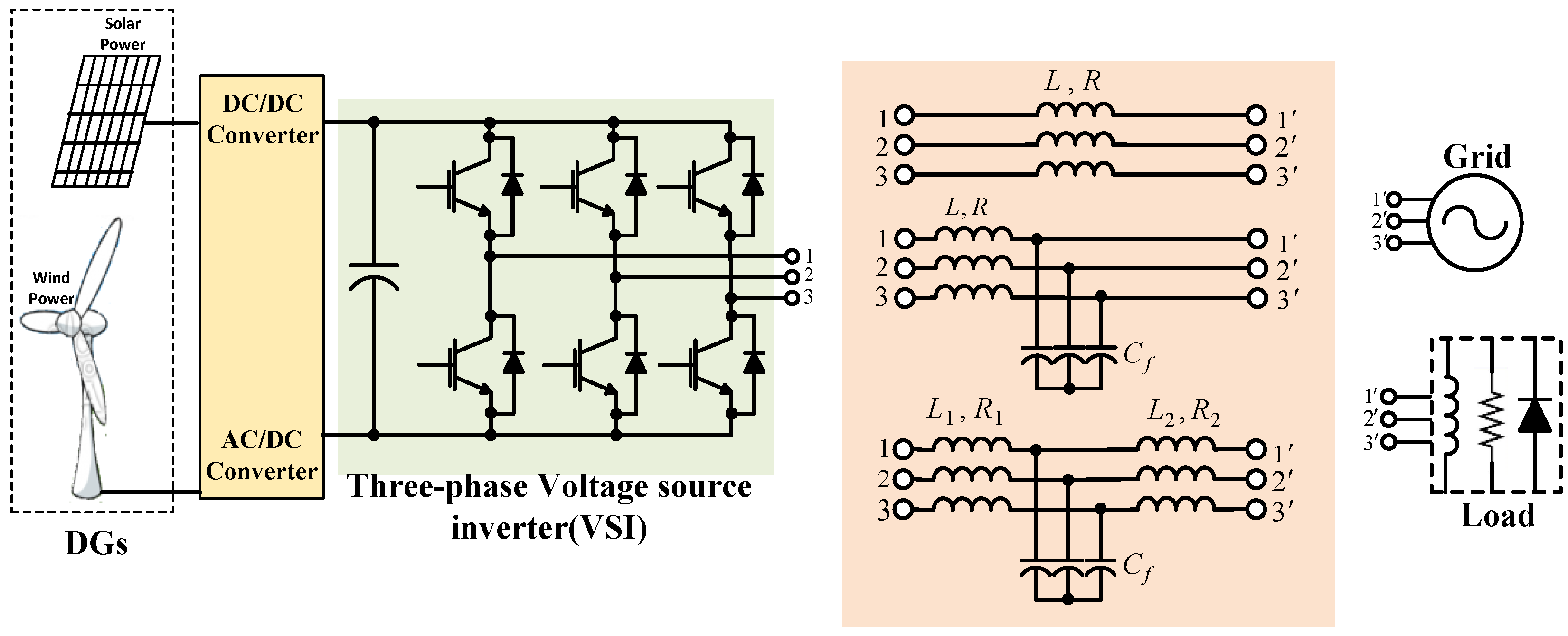
1. Introduction
- 1)
- To filter out all of the inverter output harmonics except for the fundamental frequency.
- 2)
- To have a cut off frequency much less than the switching frequency of the VSI (which typically should be lower than 0.1 of the switching frequency).
- 3)
- To limit the value of the filter inductances in order to reduce voltage drop and increase voltage transfer ratio at the rated current and also improve the voltage quality (by taking a low di/dt for large switching current ripples).
- 4)
- To minimize the total reactive power under the rated condition in order to ensure high power factor (should normally be limited to lower than 5%–10% of rated power).
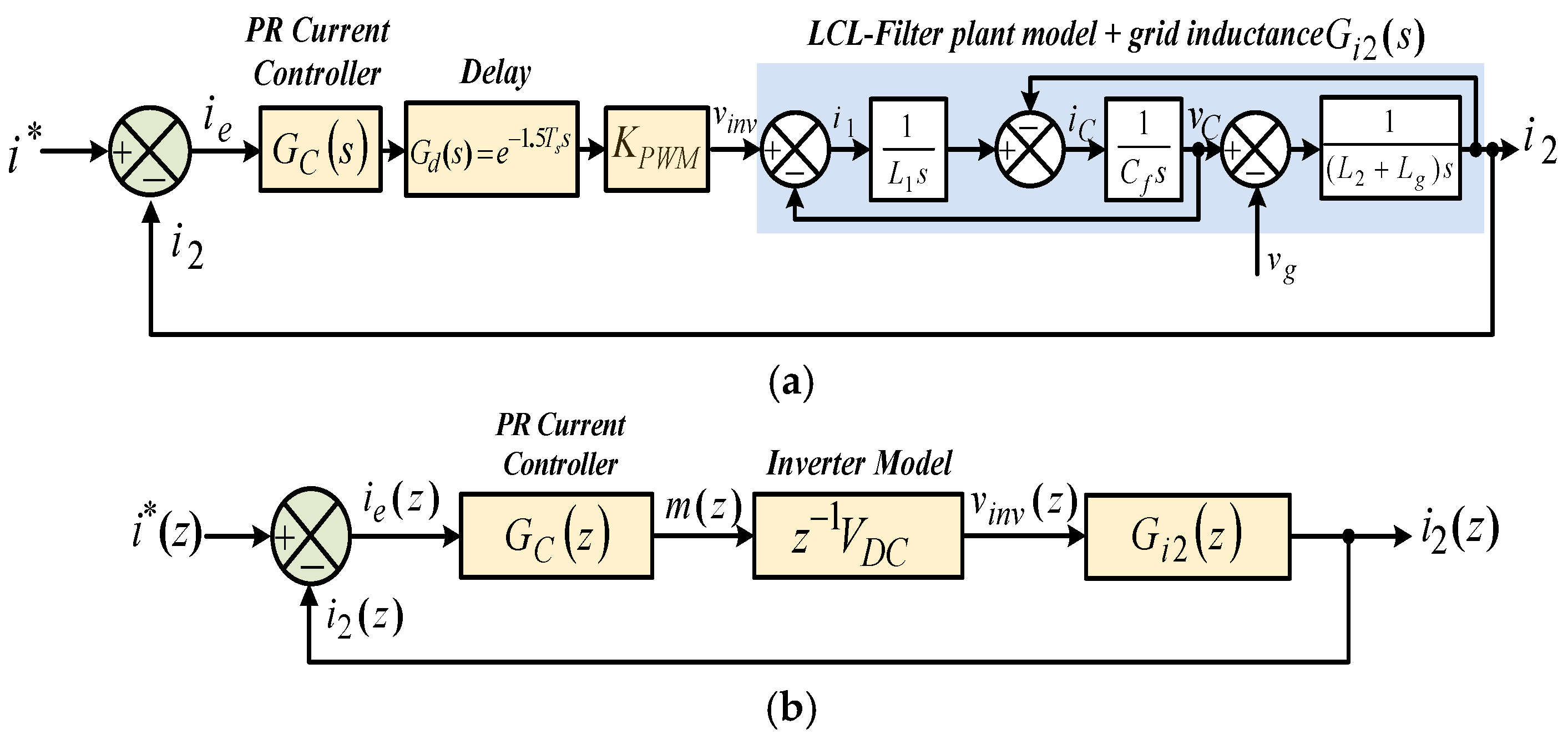
2. Stability Analysis for Single-Loop-Controlled Inductive-Capacitive-Inductive-Filtered Grid-Connected Inverter with Different Resonant Frequencies
2.1. Single-Loop Grid-Side Current Control Strategy in Discrete-Time Domain
2.1.1. System Description
2.1.2. Stability Analysis
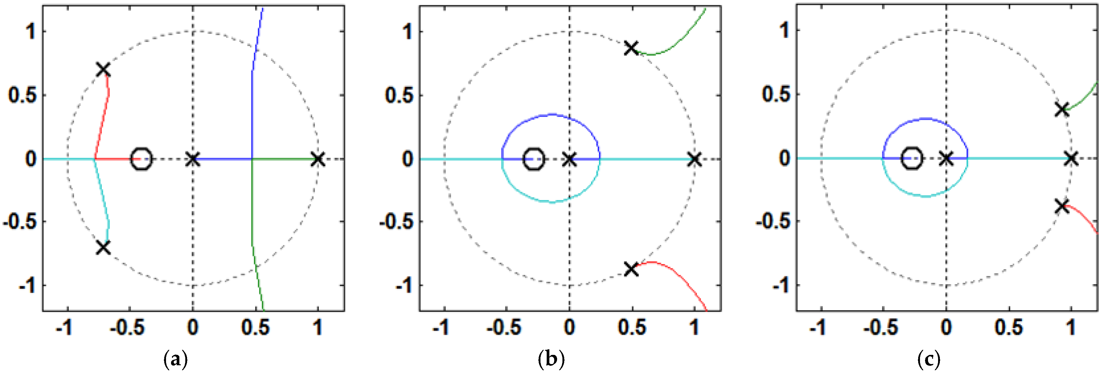
2.2. Current Controller Gains Determination for High Resonant Frequency Region
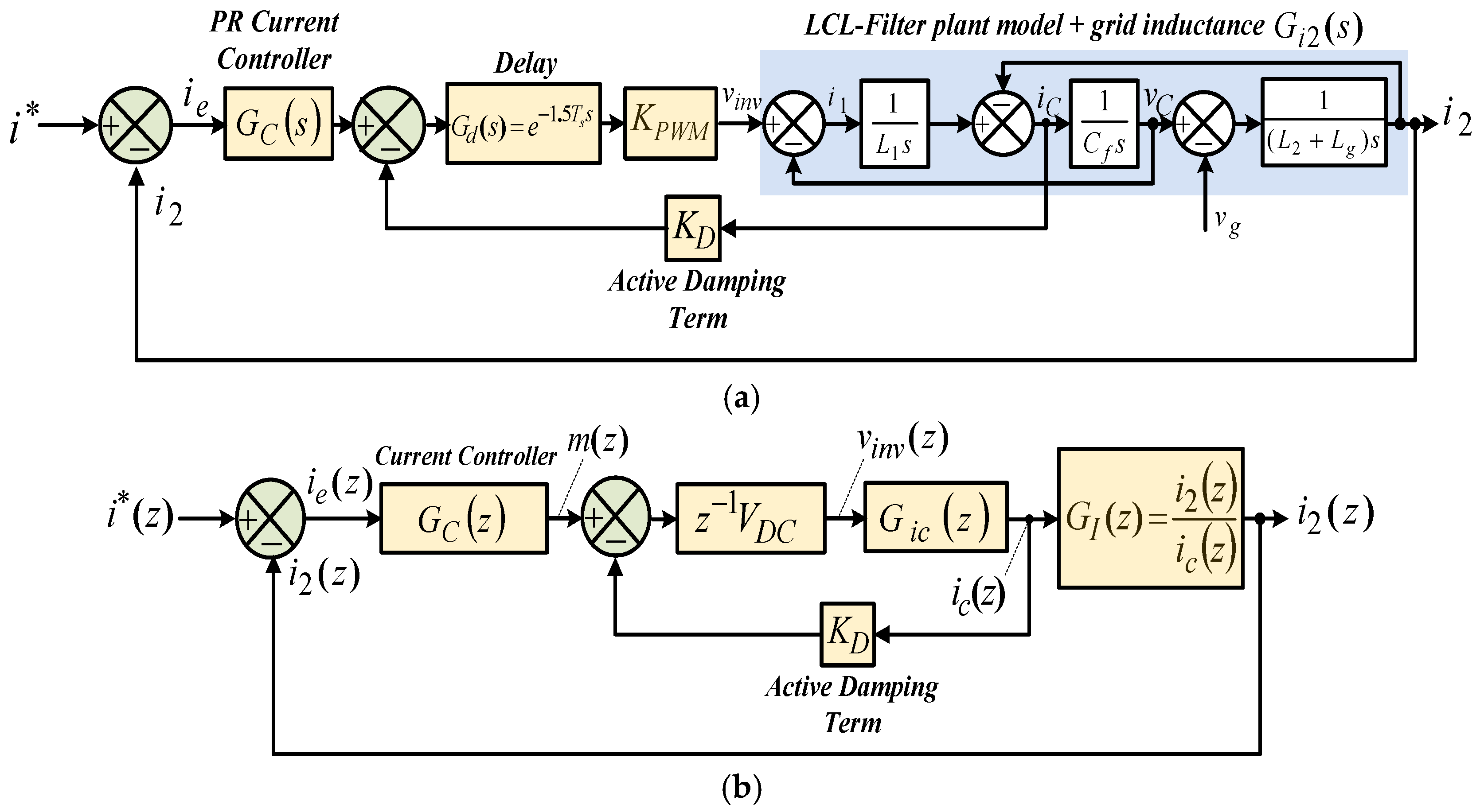
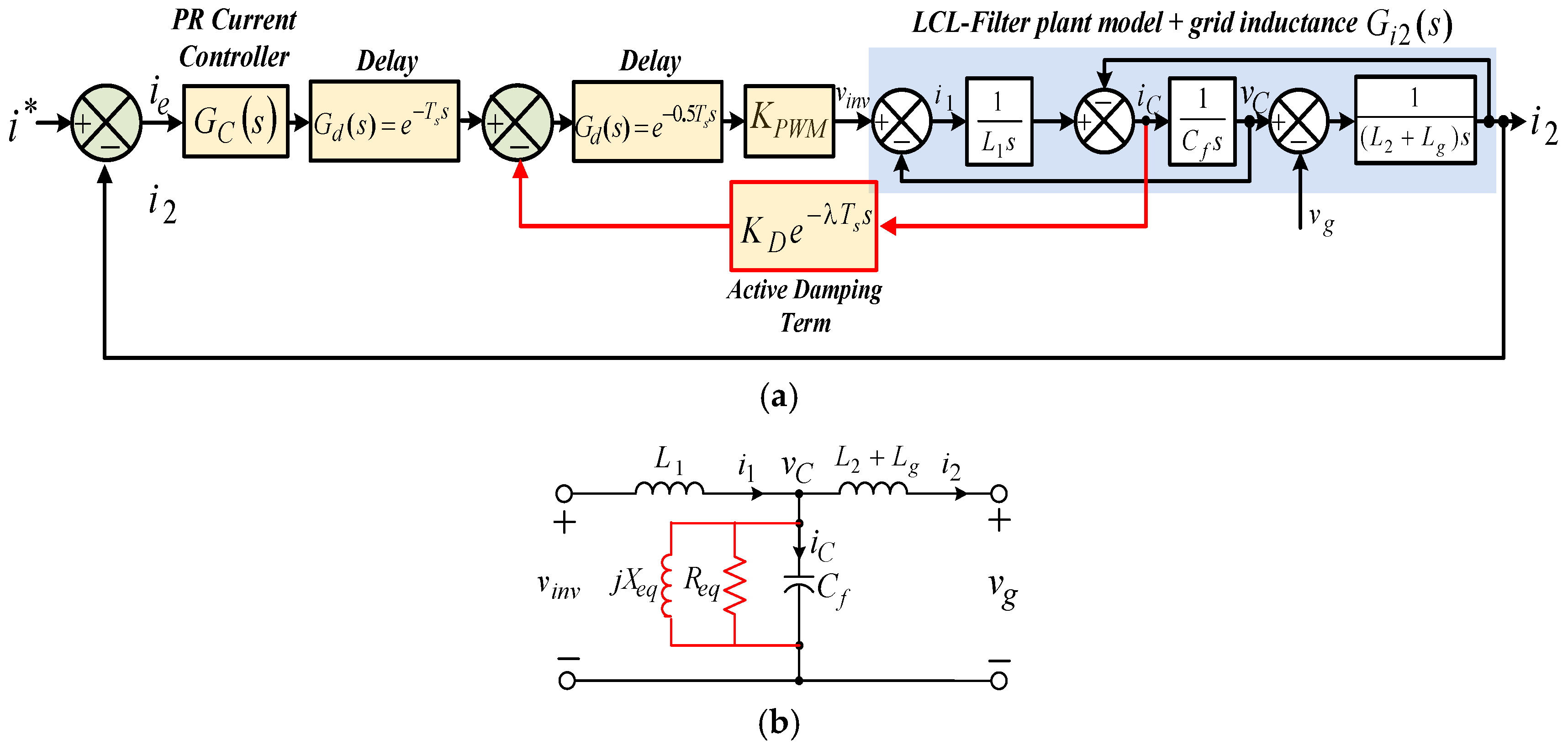
3. Proportional Capacitor Current Feedback Active Damping Approach
3.1. Impedance-Based Analysis
3.2. Computation and Pulse Width Modulation Delays Effect on the Resonance Damping Performance
- 1)
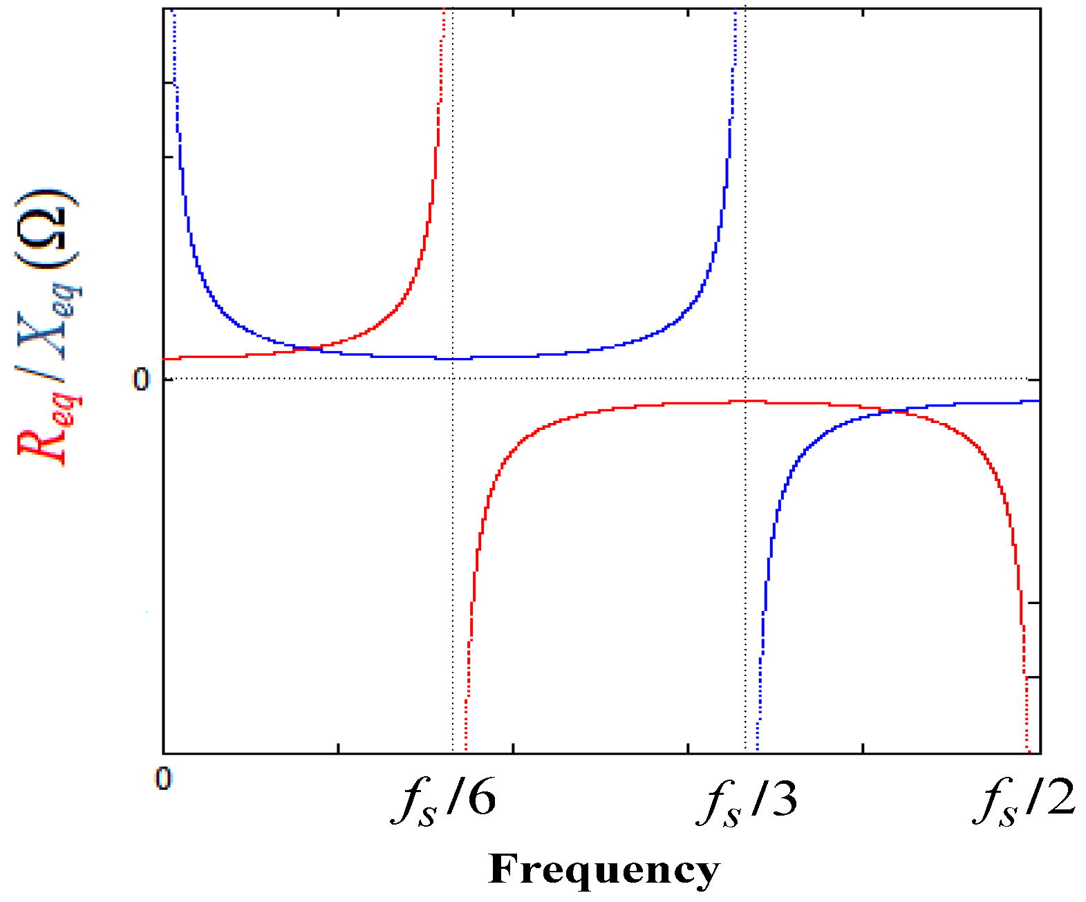
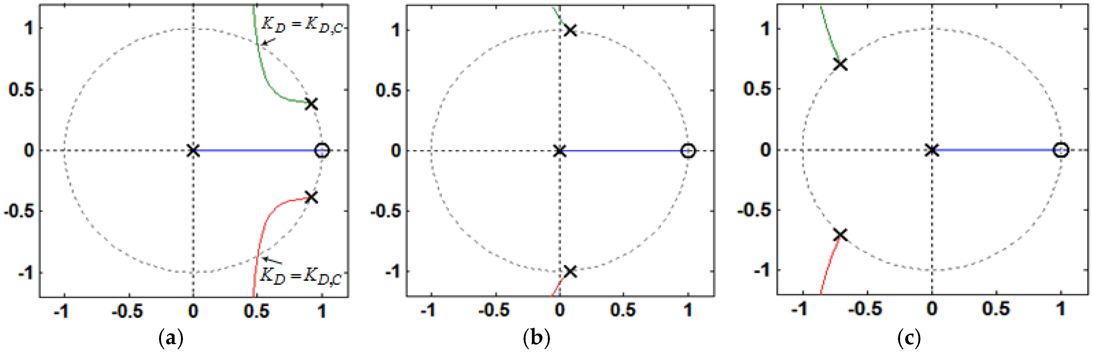
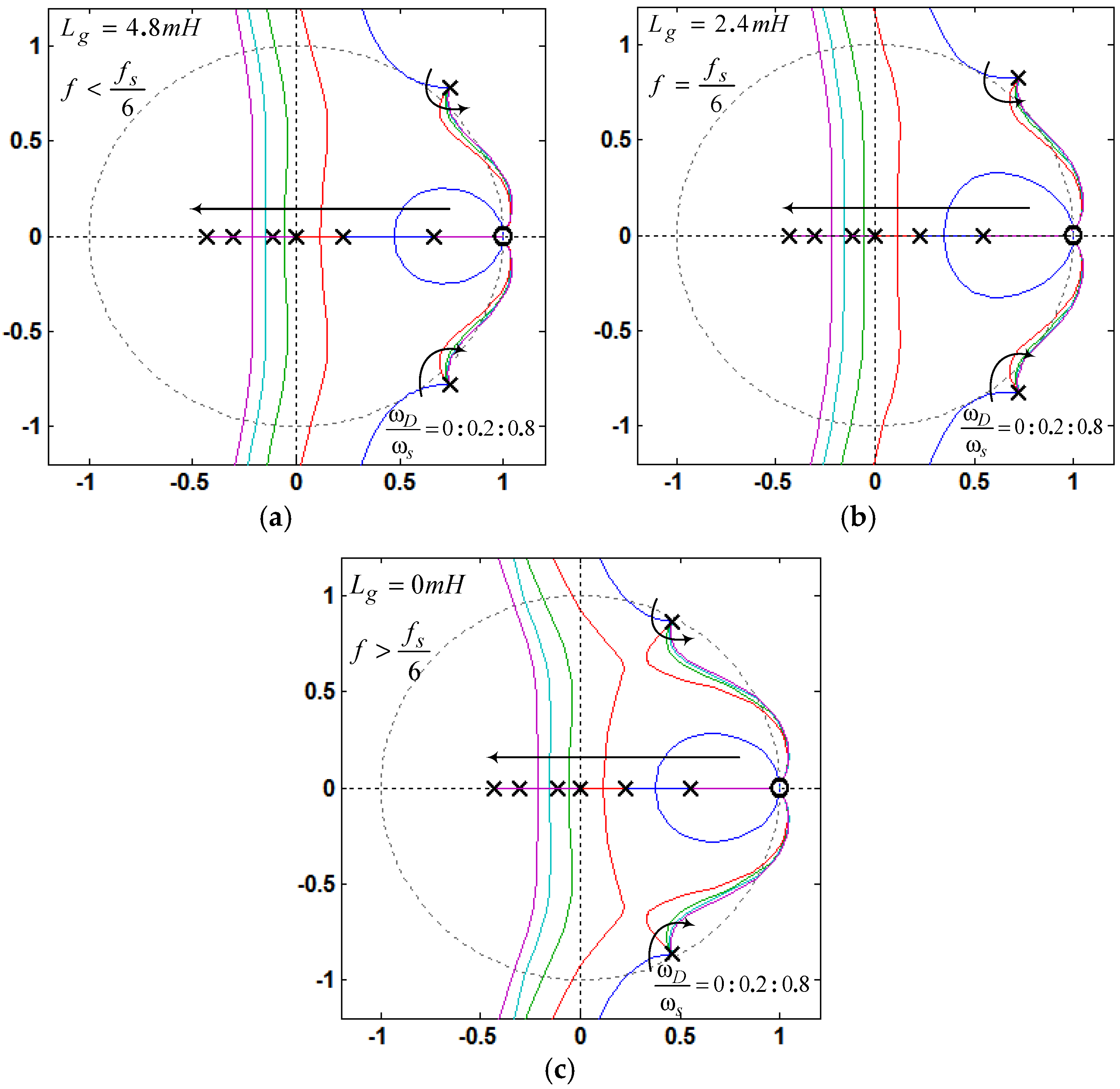
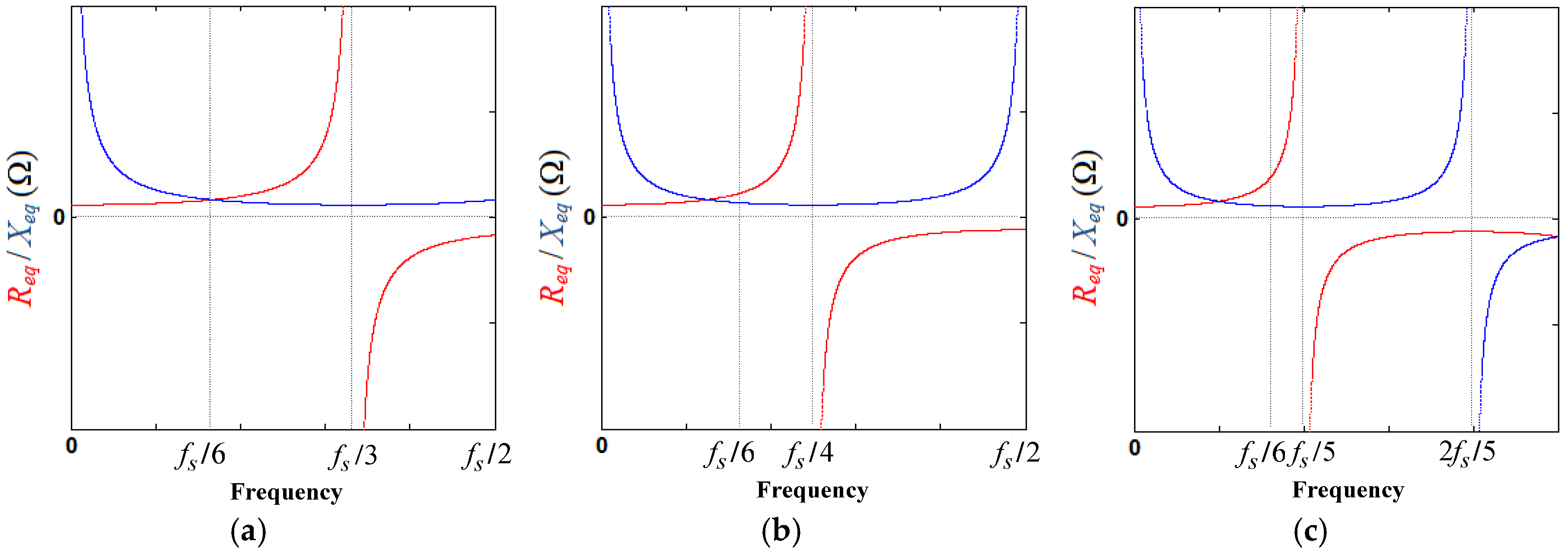
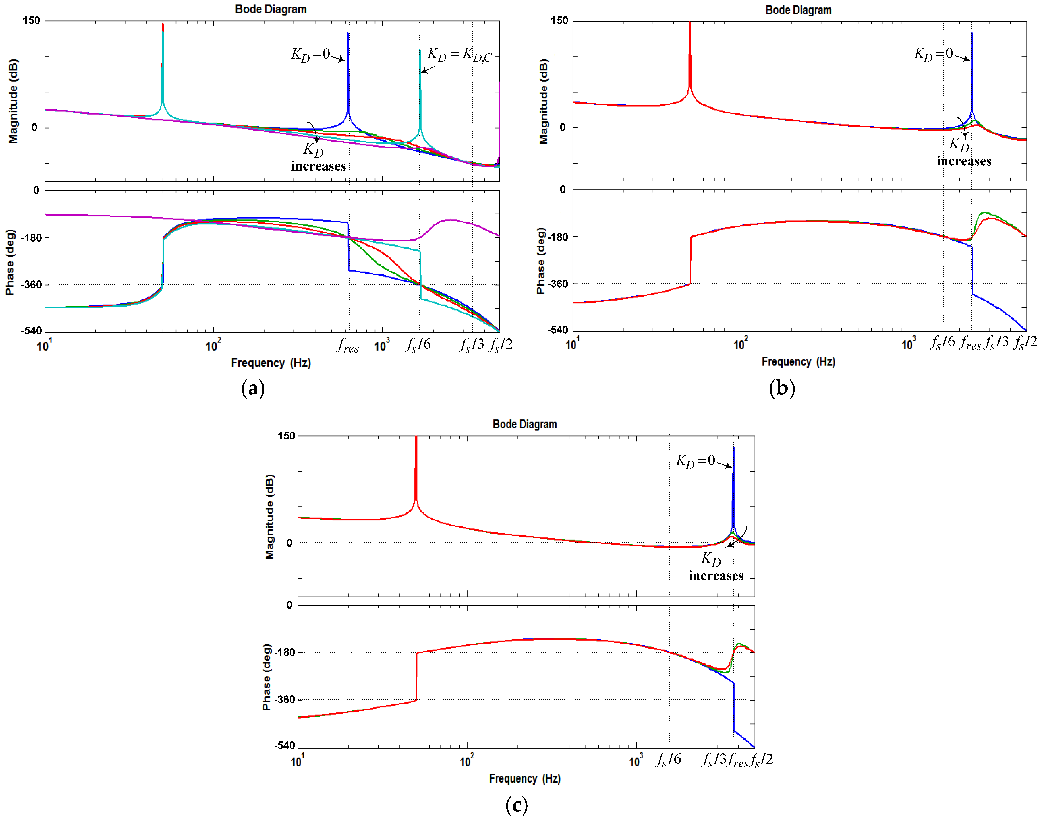
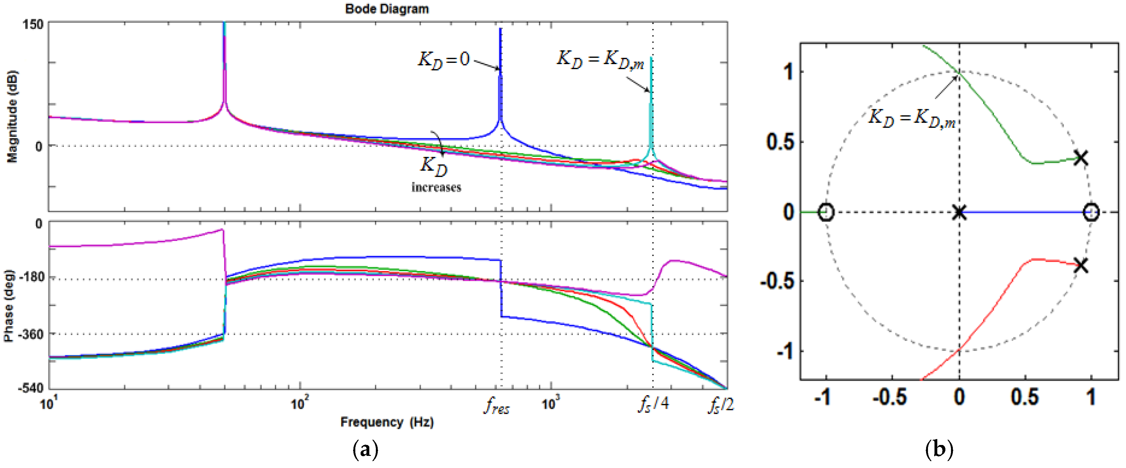
- If fres < fs/6 and 0 < KD < KD,C, i.e., < fs/6, Req is positive at (Figure 9), and no open-loop unstable poles exists, as seen in Figure 11a. Hence, the phase plot crosses over −180° only at fres in the direction of phase decrease as shown in Figure 10a. In addition, if fres < fs/6 and KD = KD,C, i.e., = fs/6, Req is infinite at (Figure 9), and no open-loop unstable poles exists, as seen in Figure 11a. In this case, it has no contribution to the resonance damping performance, and the phase plot also crosses over −180°only at fres in the direction of phase decrease (Figure 10a). As it is known well, for evaluating the stability, in the open-loop Bode diagram, the frequency ranges with amplitude above 0 dB must be investigated. In these frequency ranges, a −180° crossing in the direction of phase increase is considered as a positive crossing N+ if the gain margin at that −180° crossover frequency is smaller than 0 dB, and a −180° crossing in the direction of phase decrease is considered as a negative crossing N− if the gain margin at that −180° crossover frequency is smaller than 0 dB [42,50]. According to the Nyquist stability criterion [50], to ensure the system stability, the value of 2(N+ − N−) must be equal to the number of the open-loop unstable poles, otherwise, the system gets unstable. For fres < fs/6 and 0 < KD ≤ KD,C, i.e., ≤ fs/6, the value of (N+ − N−) is equal to zero since the gain margin at −180° crossover frequency (fres) is greater than 0 dB, as seen from Equation (34) (in dB). This means that the system will be stable in this frequency region:For KD = KD,C, Cf = 36 μF, Kp = 0.0261, and L2 = Lg = 1.8 mH, the gain margin GM1 in dB is 33.565.
- 2)
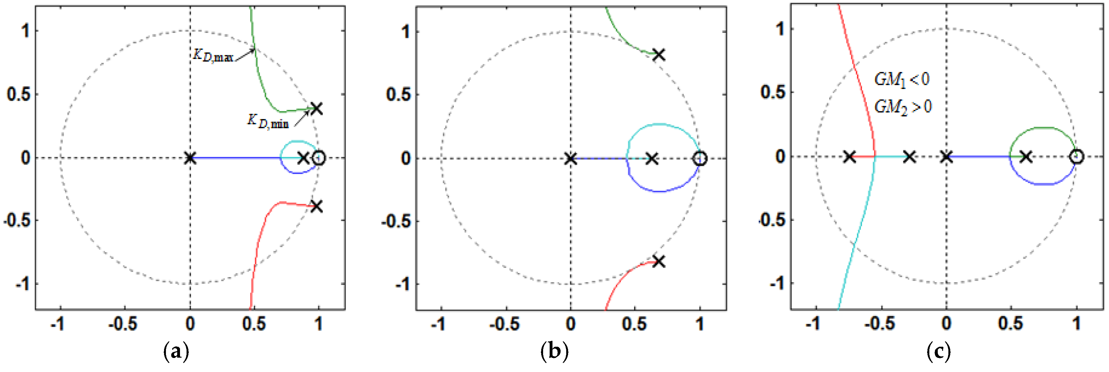
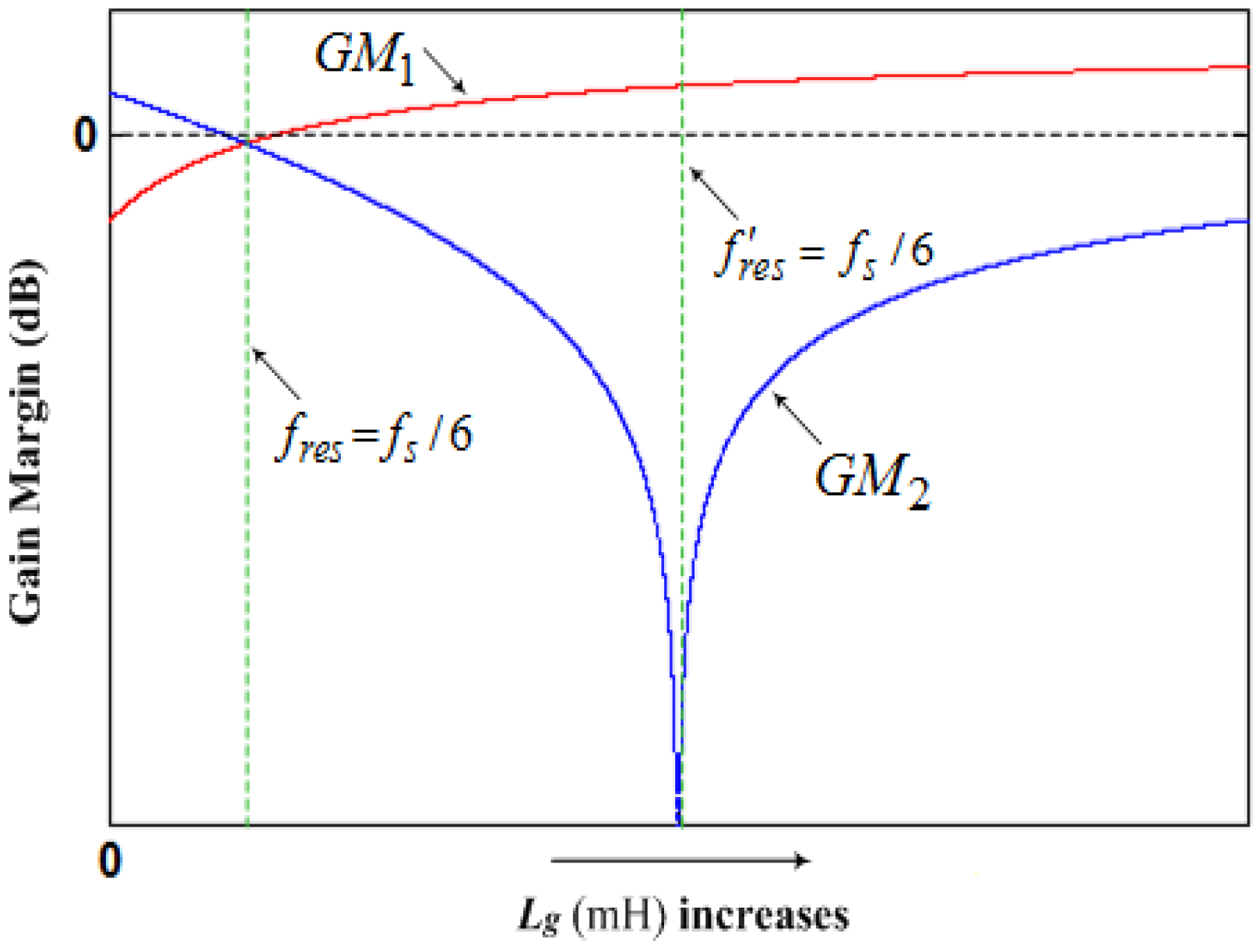
- If fres < fs/6 and KD > KD,C, i.e., > fs/6, Req is negative at (Figure 9), and a pair of open-loop unstable poles appears (non-minimum phase behavior in the closed-loop response), as seen in Figure 11a. In this case, the phase plot crosses over −180° both at fres and fs/6, respectively, in the direction of phase decrease and phase increase as shown in Figure 10a. Hence, according to the Nyquist stability criterion, to ensure the system stability, the value of 2(N+ − N−) must be equal to 2. It means that the gain margin at fres and fs/6, respectively, must be greater and smaller than 0 dB (GM1 > 0 dB and GM2 < 0 dB), i.e., N− = 0 and N+ = 1. The gain margin in dB at fs/6 can be derived from Equation (29) as Equation (35). By comparing Equations (34) and (35), one can easily understand that GM1 and GM2 will be equal, if fres = fs/6:
- 3)
- If fres ≥ fs/6 and KD > 0, i.e., > fs/6, Req is negative at (Figure 9), and a pair of open-loop unstable poles appears, as seen in Figure 11b,c. In this case, the phase plot crosses over −180° both at fs/6 and fres, respectively, in the direction of phase decrease and phase increase as seen in Figure 10b,c. Hence, to stabilize the system, GM1 < 0 dB and GM2 > 0 dB are both needed.
3.3. Robustness Evaluation Against the Grid-Impedance Variation
3.4. Current Controller and Damping Gains Determination for Low Resonant Frequency Region
4. Improved Capacitor Current Feedback Active Damping Schemes
4.1. Capacitor Current Feedback Active Damping Based on First-Order High-Pass Filter
Parameter Tunning, Stability Analysis, and Robustness Evaluation against Grid Impedance Variation
4.2. Capacitor Current Feedback Active Damping with Reduced Computation Delay
Performance of Resonance Damping with Reduced Computation Delay
5. Conclusions
Acknowledgments
Author Contributions
Conflicts of interest
References
- Carrasco, J.M.; Franquelo, L.G.; Bialasiewicz, J.T.; Galvan, E.; Guisado, R.C.P.; Prats, M.A.M.; Leon, J.I.; Moreno-Alfonso, N. Power-electronic systems for the grid integration of renewable energy sources: A survey. IEEE Trans. Ind. Electron. 2006, 53, 1002–1016. [Google Scholar] [CrossRef]
- Colak, E.; Kabalci, E.; Fulli, G.; Lazarou, S. A survey on the contributions of power electronics to smart grid systems. Renew. Sustain. Energy Rev. 2015, 47, 562–579. [Google Scholar] [CrossRef]
- Blaabjerg, F.; Teodorescu, R.; Liserre, M.; Timbus, A.V. Overview of control and grid synchronization for distributed power generation systems. IEEE Trans. Ind. Electron. 2006, 53, 1398–1409. [Google Scholar] [CrossRef]
- Bouloumpasis, I.; Vovos, P.; Georgakas, K.; Vovos, N.A. Current harmonics compensation in microgrids exploiting the power electronics interfaces of renewable energy sources. Energies 2015, 8, 2295–2311. [Google Scholar] [CrossRef]
- Langella, R.; Testa, A.; Et, A. IEEE Recommended Practice and Requirements for Harmonic Control in Electric Power System; IEEE Std. 519-1992/2014; IEEE Standards Association: New York, NY, USA, 2014. [Google Scholar]
- IEEE Guide—Adoption of IEC/TR 61000-3-7:2008, Electromagnetic Compatibility (EMC)—Limits—Assessment of Emission Limits for the Connection of Fluctuating Installations to MV, HV, and EHV Power Systems; IEEE Standards Association: New York, NY, USA, 2012.
- Liserre, M.; Blaabjerg, F.; Hansen, S. Design and control of an LCL-filter-based three-phase active rectifier. IEEE Trans. Ind. Appl. 2005, 41, 1281–1291. [Google Scholar] [CrossRef]
- Gabe, I.J.; Montagner, V.F.; Pinheiro, H. Design and implementation of a robust current controller for VSI connected to the grid through an LCL-filter. IEEE Trans. Power Electron. 2009, 24, 1444–1452. [Google Scholar] [CrossRef]
- Dannehl, J.; Wessels, C.; Fuchs, F.W. Limitations of voltage-oriented PI current control of grid-connected PWM rectifiers with LCL filters. IEEE Trans. Ind. Electron. 2009, 56, 380–388. [Google Scholar] [CrossRef]
- Loh, P.C.; Holmes, D.G. Analysis of multiloop control strategies for LC/CL/LCL-filtered voltage-source and current-source inverters. IEEE Trans. Ind. Appl. 2005, 41, 644–654. [Google Scholar] [CrossRef]
- Tang, Y.; Loh, P.C.; Wang, P.; Choo, F.H.; Gao, F. Exploring inherent damping characteristic of LCL-Filters for three-phase grid-connected. IEEE Trans. Power Electron. 2012, 27, 1433–1442. [Google Scholar] [CrossRef]
- Savaghebi, M.; Jalilian, A.; Vasquez, J.C.; Guerrero, J.M. Secondary control scheme for voltage unbalance compensation in an islanded droop-controlled microgrid. IEEE Trans. Smart Grid 2012, 3, 797–807. [Google Scholar] [CrossRef]
- Blasko, V.; Kaura, V. A novel control to actively damp resonance in input LC filter of a three-phase voltage source converter. IEEE Trans. Ind. Appl. 1997, 33, 542–550. [Google Scholar] [CrossRef]
- Tang, Y.; Loh, P.C.; Wang, P.; Choo, F.H.; Tan, K.K. Improved one cycle-control scheme for three-phase active rectifiers with input inductor capacitor-inductor filters. IET Power Electron. 2011, 4, 603–614. [Google Scholar] [CrossRef]
- Jalili, K.; Bernet, S. Design of LCL-filters of active-front-end two-level voltage-source converters. IEEE Trans. Ind. Electron. 2009, 56, 1674–1689. [Google Scholar] [CrossRef]
- Rockhill, A.A.; Liserre, M.; Teodorescu, R.; Rodriguez, P. Grid-filter design for a multi-megawatt medium-voltage voltage-source inverter. IEEE Trans. Ind. Electron. 2011, 58, 1205–1217. [Google Scholar] [CrossRef] [Green Version]
- Cao, W.; Liu, K.; Ji, Y.; Wang, Y.; Zhao, J. Design of a four-branch LCL-type grid-connecting interface for a three-phase, four-leg active power filter. Energies 2015, 8, 1606–1627. [Google Scholar] [CrossRef]
- Shen, G.; Xu, D.; Cao, L.; Zhu, X. An improved control strategy for grid-connected voltage source inverters with an LCL filter. IEEE Trans. Power Electron. 2008, 23, 1899–1906. [Google Scholar] [CrossRef]
- Shen, G.; Zhu, X.; Zhang, J.; Xu, D. A new feedback method for PR current control of LCL-filter-based grid-connected inverter. IEEE Trans. Ind. Electron. 2010, 57, 2033–2041. [Google Scholar] [CrossRef]
- He, N.; Xu, D.; Zhu, Y.; Zhang, J.; Shen, G.; Zhang, Y.; Ma, J.; Liu, C. Weighted average current control in a three-phase grid inverter with an LCL filter. IEEE Trans. Power Electron. 2013, 28, 2785–2797. [Google Scholar] [CrossRef]
- Twining, E.; Holmes, D.G. Grid current regulation of a three-phase voltage source inverter with an LCL input filter. IEEE Trans. Power Electron. 2003, 18, 888–895. [Google Scholar] [CrossRef]
- Dannehl, J.; Fuchs, F.W.; Hansen, S.; Thogersen, P.B. Investigation of active damping approaches for PI-based current control of grid-connected pulse width modulation converters with LCL filters. IEEE Trans. Ind. Appl. 2010, 46, 1509–1517. [Google Scholar] [CrossRef]
- Parker, S.G.; McGrath, B.P.; Holmes, D.G. Regions of active damping control for LCL filters. IEEE Trans. Ind. Appl. 2014, 50, 424–432. [Google Scholar] [CrossRef]
- Buso, S.; Mattavelli, P. Digital Control in Power Electronics; Morgan and Claypool: San Rafael, CA, USA, 2006. [Google Scholar]
- Holmes, D.G.; Lipo, T.A.; McGrath, B.P.; Kong, W.Y. Optimized design of stationary frame three phase AC current regulators. IEEE Trans. Power Electron. 2009, 24, 2417–2426. [Google Scholar] [CrossRef]
- Li, X.; Wu, X.; Geng, Y.; Yuan, X.; Xia, C.; Zhang, X. Wide damping region for LCL-type grid-connected inverter with an improved capacitor-current-feedback method. IEEE Trans. Power Electron. 2015, 30, 5247–5259. [Google Scholar] [CrossRef]
- Bao, C.; Ruan, X.; Wang, X.; Li, W.; Pan, D.; Weng, K. Step-by-step controller design for LCL-type grid-connected inverter with capacitor-current-feedback active damping. IEEE Trans. Power Electron. 2014, 29, 1239–1253. [Google Scholar]
- Channegowda, P.; John, V. Filter optimization for grid interactive voltage source inverters. IEEE Trans. Ind. Electron. 2010, 57, 4106–4114. [Google Scholar] [CrossRef]
- Pena-Alzola, R.; Liserre, M.; Blaabjerg, F.; Sebastian, R.; Dannehl, J.; Fuchs, F.W. Analysis of the passive damping losses in LCL-filter-based grid converters. IEEE Trans. Power Electron. 2013, 28, 2642–2646. [Google Scholar] [CrossRef]
- Wu, W.; He, Y.; Blaabjerg, F. An LLCL-power filter for single-phase grid-tied inverter. IEEE Trans. Power Electron. 2012, 27, 782–789. [Google Scholar] [CrossRef]
- Wu, W.; He, Y.; Tang, T.; Blaabjerg, F. A new design method for the passive damped LCL and LLCL filter-based single-phase grid-tied inverter. IEEE Trans. Ind. Electron. 2013, 60, 4339–4350. [Google Scholar] [CrossRef]
- Wu, W.; Sun, Y.; Huang, M.; Wang, X.; Blaabjerg, F.; Liserre, M.; Chung, H.S. A robust passive damping method for LLCL-filter-based grid-tied inverters to minimize the effect of grid harmonic voltages. IEEE Trans. Power Electron. 2014, 29, 3279–3289. [Google Scholar] [CrossRef]
- Beres, R.N.; Wang, X.; Blaabjerg, F.; Bak, C.L.; Liserre, M. A Review of Passive Filters for Grid-Connected Voltage Source Converters. In Proceedings of the IEEE Applied Power Electronics Conference and Exposition, Fort Worth, TX, USA, 16–20 March 2014; pp. 2208–2215.
- Dannehl, J.; Liserre, M.; Fuchs, F.W. Filter-based active damping of voltage source converters with LCL filter. IEEE Trans. Ind. Electron. 2011, 58, 3623–3633. [Google Scholar] [CrossRef]
- Xu, J.; Xie, S.; Tang, T. Active damping-based control for grid-connected LCL-filtered inverter with injected grid current feedback only. IEEE Trans. Ind. Electron. 2014, 61, 4746–4758. [Google Scholar] [CrossRef]
- Wang, X.; Blaabjerg, F.; Loh, P.C. Grid-current-feedback active damping for LCL resonance in grid-connected voltage-source converters. IEEE Trans. Power Electron. 2016, 31, 213–223. [Google Scholar] [CrossRef]
- He, J.; Li, Y.W. Generalized closed-loop control schemes with embedded virtual impedances for voltage source converters with LC or LCL filters. IEEE Trans. Power Electron. 2012, 27, 1850–1861. [Google Scholar] [CrossRef]
- Liu, F.; Duan, S.; Yin, J.; Liu, B.; Liu, F. Parameter design of a two current-loop controller used in a grid-connected inverter system with LCL filter. IEEE Trans. Ind. Electron. 2009, 56, 4483–4491. [Google Scholar]
- Li, Y.W. Control and resonance damping of voltage source and current source converters with LC filters. IEEE Trans. Ind. Electron. 2009, 56, 1511–1521. [Google Scholar]
- Wessels, C.; Dannehl, J.; Fuchs, F. Active Damping of LCL-Filter Resonance Based on Virtual Resistor for PWM Rectifiers-Stability Analysis with Different Filter Parameters. In Proceedings of the IEEE Power Electronic Specialists Conference, Rhodes, Greece, 15–19 June 2008; pp. 3532–3538.
- Jia, Y.; Zhao, J.; Fu, X. Direct grid current control of LCL-filtered grid-connected inverter mitigating grid voltage disturbance. IEEE Trans. Power Electron. 2014, 29, 1532–1541. [Google Scholar]
- Pan, D.; Ruan, X.; Bao, C.; Li, W.; Wang, X. Capacitor-current-feedback active damping with reduced computation delay for improving robustness of LCL-type grid-connected inverter. IEEE Trans. Power Electron. 2014, 29, 3414–3427. [Google Scholar] [CrossRef]
- Zou, Z.; Wang, Z.; Cheng, M. Modeling, analysis, and design of multifunction grid-interfaced inverters with output LCL filter. IEEE Trans. Power Electron. 2014, 29, 3830–3839. [Google Scholar] [CrossRef]
- Tang, Y.; Loh, P.C.; Wang, P.; Choo, F.H.; Gao, F.; Blaabjerg, F. Generalized design of high performance shunt active power filter with output LCL filter. IEEE Trans. Ind. Electron. 2012, 59, 1443–1452. [Google Scholar] [CrossRef]
- Wang, X.; Blaabjerg, F.; Loh, P.C. Design-Oriented Analysis of Resonance Damping and Harmonic Compensation for LCL-Filtered Voltage Source Converters. In Proceedings of the IEEE International Power Electronics Conference, Hiroshima, Japan, 18–21 May 2014; pp. 216–223.
- Pan, D.; Ruan, X.; Bao, C.; Li, W.; Wang, X. Optimized controller design for LCL-type grid-connected inverter to achieve high robustness against grid-impedance variation. IEEE Trans. Ind. Electron. 2015, 62, 1537–1547. [Google Scholar] [CrossRef]
- Sung-Yeul, P.; Chen, C.; Jih-Sheng, L.; Seung-Ryul, M. Admittance compensation loop control for a grid-tie LCL fuel cell inverter. IEEE Trans. Power Electron. 2008, 23, 1716–1723. [Google Scholar] [CrossRef]
- Harnefors, L.; Bongiorno, M.; Lundberg, S. Input-admittance calculation and shaping for controlled voltage-source converters. IEEE Trans. Ind. Electron. 2007, 54, 3323–3334. [Google Scholar] [CrossRef]
- Messo, T.; Jokipii, J.; Makinen, A.; Suntio, T. Modeling the Grid Synchronization Induced Negative-Resistor-Like Behavior in the Output Impedance of A Three-Phase Photovoltaic Inverter. In Proceedings of the 2013 4th IEEE International Symposium on Power Electronics for Distributed Generation Systems (PEDG), Rogers, AR, USA, 8–11 July 2013; pp. 1–7.
- Goodwin, G.C.; Graebe, S.F.; Salgado, M.E. Control. System Design; Universidad Tecnica Federico Santa Maria: Valparaiso, Chile, 2000. [Google Scholar]
- Yepes, A.G.; Freijedo, F.D.; Lopez, O.; Gandoy, J. High-performance digital resonant controllers implemented with two integrators. IEEE Trans. Power Electron. 2011, 26, 563–576. [Google Scholar] [CrossRef]
- Pogaku, N.; Green, T.C. Harmonic mitigation throughout a distribution system: A distributed-generator-based solution. IEE Proc. Gener. Transmiss. Distrib. 2006, 153, 350–358. [Google Scholar] [CrossRef]
- Wang, X.; Blaabjerg, F.; Loh, P.C. Virtual RC damping of LCL-filtered voltage source converters with extended selective harmonic compensation. IEEE Trans. Power Electron. 2015, 30, 4726–4737. [Google Scholar] [CrossRef]
- Liserre, M.; Aquilu, A.D.; Blaabjerg, F. Genetic algorithm-based design of the active damping for an LCL-filter three-phase active rectifier. IEEE Trans. Power Electron. 2004, 19, 76–86. [Google Scholar] [CrossRef]
- Liserre, M.; Teodorescu, R.; Blaabjerg, F. Stability of photovoltaic and wind turbine grid-connected inverters for a large set of grid impedance values. IEEE Trans. Power Electron. 2006, 21, 263–272. [Google Scholar] [CrossRef]
- Sun, J. Impedance-based stability criterion for grid-connected inverters. IEEE Trans. Power Electron. 2011, 26, 3075–3078. [Google Scholar] [CrossRef]
- Yin, J.; Duan, S.; Liu, B. Stability analyses of grid-connected inverter with LCL filter adopting a digital single-loop controller with inherent damping characteristic. IEEE Trans. Ind. Inf. 2013, 9, 1104–1112. [Google Scholar] [CrossRef]
- Pena-Alzola, R.; Liserre, M.; Blaabjerg, F.; Sebastian, R.; Dannehl, J.; Fuchs, F.W. Systematic design of the lead-lag network method for active damping in LCL-filter based three-phase converters. IEEE Trans. Ind. Inf. 2014, 10, 43–52. [Google Scholar] [CrossRef]
- Malinowski, M.; Bernet, S. A simple voltage sensor-less active damping scheme for three-phase PWM converters with an LCL-filter. IEEE Trans. Ind. Electron. 2008, 55, 1876–1880. [Google Scholar] [CrossRef]
- Liu, C.; Zhang, X.; Tan, L.H.; Liu, F. A Novel Control Strategy of LCL-VSC Based on Notch Concept. In Proceedings of the IEEE International Symposium on Power Electronics for Distributed Generation Systems, Hefei, China, 16–18 June 2010; pp. 343–346.


| System Parameters | L1 = 3.6 mH | L2 = 1.8 mH | Lg =1.8 mH |
| Ts = 1/fs = 100 μs (Sampling Period) | ω0 = 100π | 2VDC = 650 V | fsw = 5 kHz |
| Filter Capacitances and Resonance Frequencies | Cf = 36 μF | fres = 0.625 kHz | fres/fs = 0.0625 |
| Cf = 5 μF | fres = 1.67 kHz | fres/fs = 0.167 | |
| Cf = 1 μF | fres = 3.751 kHz | fres/fs = 0.3751 |
© 2016 by the authors; licensee MDPI, Basel, Switzerland. This article is an open access article distributed under the terms and conditions of the Creative Commons Attribution (CC-BY) license (http://creativecommons.org/licenses/by/4.0/).
Share and Cite
Lorzadeh, I.; Askarian Abyaneh, H.; Savaghebi, M.; Bakhshai, A.; Guerrero, J.M. Capacitor Current Feedback-Based Active Resonance Damping Strategies for Digitally-Controlled Inductive-Capacitive-Inductive-Filtered Grid-Connected Inverters. Energies 2016, 9, 642. https://doi.org/10.3390/en9080642
Lorzadeh I, Askarian Abyaneh H, Savaghebi M, Bakhshai A, Guerrero JM. Capacitor Current Feedback-Based Active Resonance Damping Strategies for Digitally-Controlled Inductive-Capacitive-Inductive-Filtered Grid-Connected Inverters. Energies. 2016; 9(8):642. https://doi.org/10.3390/en9080642
Chicago/Turabian StyleLorzadeh, Iman, Hossein Askarian Abyaneh, Mehdi Savaghebi, Alireza Bakhshai, and Josep M. Guerrero. 2016. "Capacitor Current Feedback-Based Active Resonance Damping Strategies for Digitally-Controlled Inductive-Capacitive-Inductive-Filtered Grid-Connected Inverters" Energies 9, no. 8: 642. https://doi.org/10.3390/en9080642