Article

Analysis and Modeling for Short- to Medium-Term Load Forecasting Using a Hybrid Manifold Learning Principal Component Model and Comparison with Classical Statistical Models (SARIMAX, Exponential Smoothing) and Artificial Intelligence Models (ANN, SVM): The Case of Greek Electricity Market

by
George P. Papaioannou
1,2,
Christos Dikaiakos
1,3,*,†,
Anargyros Dramountanis
3,† and
Panagiotis G. Papaioannou
4,†
1
Research, Technology & Development Department, Independent Power Transmission Operator (IPTO) S.A., 89 Dyrrachiou & Kifisou Str. Gr, Athens 10443, Greece
2
Center for Research and Applications in Nonlinear Systems (CRANS), Department of Mathematics, University of Patras, Patras 26500, Greece
3
Department of Electrical and Computer Engineering, University of Patras, Patras 26500, Greece
4
Applied Mathematics and Physical Sciences, National Technical University of Athens, Zografou 15780, Greece
*
Author to whom correspondence should be addressed.
These authors contributed equally to this work.
Energies 2016, 9(8), 635; https://doi.org/10.3390/en9080635
Submission received: 22 April 2016 / Revised: 5 July 2016 / Accepted: 27 July 2016 / Published: 16 August 2016

Abstract

:
In this work we propose a new hybrid model, a combination of the manifold learning Principal Components (PC) technique and the traditional multiple regression (PC-regression), for short and medium-term forecasting of daily, aggregated, day-ahead, electricity system-wide load in the Greek Electricity Market for the period 2004–2014. PC-regression is shown to effectively capture the intraday, intraweek and annual patterns of load. We compare our model with a number of classical statistical approaches (Holt-Winters exponential smoothing of its generalizations Error-Trend-Seasonal, ETS models, the Seasonal Autoregressive Moving Average with exogenous variables, Seasonal Autoregressive Integrated Moving Average with eXogenous (SARIMAX) model as well as with the more sophisticated artificial intelligence models, Artificial Neural Networks (ANN) and Support Vector Machines (SVM). Using a number of criteria for measuring the quality of the generated in-and out-of-sample forecasts, we have concluded that the forecasts of our hybrid model outperforms the ones generated by the other model, with the SARMAX model being the next best performing approach, giving comparable results. Our approach contributes to studies aimed at providing more accurate and reliable load forecasting, prerequisites for an efficient management of modern power systems.

Graphical Abstract

1. Introduction

The unique characteristic of electricity is that it cannot be stored. In order to achieve frequency stability energy production must be equal to the instantaneously consumed production. Considering also the physical constraints that impose limitations (congestion) on the power transferred in transmission lines we can realize why competitive pricing is not easy to implement in real-time markets.
Today energy markets’ products are defined in terms of delivering a predetermined amount of power over a specified period of time. These markets are usually called spot markets where the prices (spots) are determined within one hour or half an hour time periods (e.g., Australia). Spot prices emerge either from auctions which take place in the so-called market pool, where retailers and generators’ representatives make offers and bids or from trading on an exchange platform either in the day-ahead or in the real-time market [1,2,3]. The market clearing price is therefore determined by the most expensive unit dispatched in the abovementioned mechanisms over the respective trading period. The key factors that influence spot prices are mainly the demand or load as well as the ability to respond to this demand by the available generating units. Therefore, possible errors in load forecasting could have significant cost implications for the market participants. More specifically an underestimated predicted load could lead to unavailability the required reserve margin which in turn could lead to high costs from peak units. On the other hand, load overestimations would cause the problem of excess supply management pushing spot prices downwards.
Load prediction is a complex procedure because of the nature of the influencing factors—weather factors, seasonal factors and social-economic factors [4]. Weather factors include temperature, relative humidity, wind speed, dew point, etc. Seasonal factors include climate variation during a year while social-economic factors are depicted through periodicities inside the time-series of the load as well as trends through years.
An electricity utility also can use forecasts in making important decisions related to purchasing and generating electric power, load switching and investing in infrastructure development. Also, energy suppliers, financial institutions and other “players” in the electric energy generation and distribution markets can benefit from reliable load forecasting.
Load is a variable that is affected by a large number of factors whose influences are “imprinted” in its dynamic evolution. Its historical past values, weather data, the clustering of customers according to their consumption profiles, the number of types of electric appliances in a given region as well as consumer age, economic and demographic data and their evolution in the future, are some of the crucial factors taken into account in medium and long-term load forecasting.
Also, the time of the year, the day of the week and the hour of the day are time factors that must be included in load forecasting. The consumption of electricity for example in Mondays, Fridays, or holidays etc. is different. Load is also strongly influenced by weather conditions. In a survey performed in 2001 bu Hippert et al. [5], in out of 22 research papers, 13 only considered temperature, indicating the significance of this meteorological parameter in load forecasting. In this work, we have included the average temperature in the country, as a predictor, in the seasonal Auto-Regressive Integrated Moving Average (ARIMA) model for load forecasting.
Load forecasting is also a necessary tool for Transmission System Operators (TSOs) since it is used for different purposes and on different time scales. Short-term forecasts (one hour–one week) are useful for dispatchers to schedule short-term maintenance, unit commitment, fuel allocation, and cross-border trade, but also to operation engineers for network feature analysis such as optimal power flow, etc. Medium term forecasts (one week–one month) are used by TSOs for planning and operation of the power system while long-term forecasts (one month–years) are required for capacity planning and maintenance scheduling.
In this sense, load forecasting is of crucial importance for the operation and management of power systems and thus has been a major field of research in energy markets. There exist many statistical methods which are implemented to predict the behavior of electricity loads, with varying success under different market conditions [6]. In this approach, the load pattern is treated as a time series signal, where various time series techniques are applied. The most common approach is the Box-Jenkins’ Auto-Regressive Integrated Moving Average (ARIMA) [7] model and its generalized form Seasonal ARIMA with eXogenous parameters (SARIMAX) [8,9]. Models utilized in electricity load forecasting also include reg-ARIMA, a regressive ARIMA model, Principal Component Analysis and Holt-Winters exponential smoothing [10,11,12]. All of the abovementioned methods are structured in such a way in order to deal with the double seasonality (intraday and intraweek cycles) inherent in load data.
Neural Networks (NNs) and Artificial Neural Networks (ANNs) [13,14] are considered to be other more advanced forecasting methods. ANNs are useful for multivariate modeling but have not been reported to be so effective in univariate short-term prediction. However, the complexity of the latter and their questionable performance has relegated NNs and ANNs to being perhaps considered the last resort solution to any forecasting problem [15]. State space and Kalman filtering technologies have thus far proved to be one of the most complex, yet reliable methods in time series forecasting [16,17]. A number of different load forecasting methods have been developed over the last few decades, as described below.
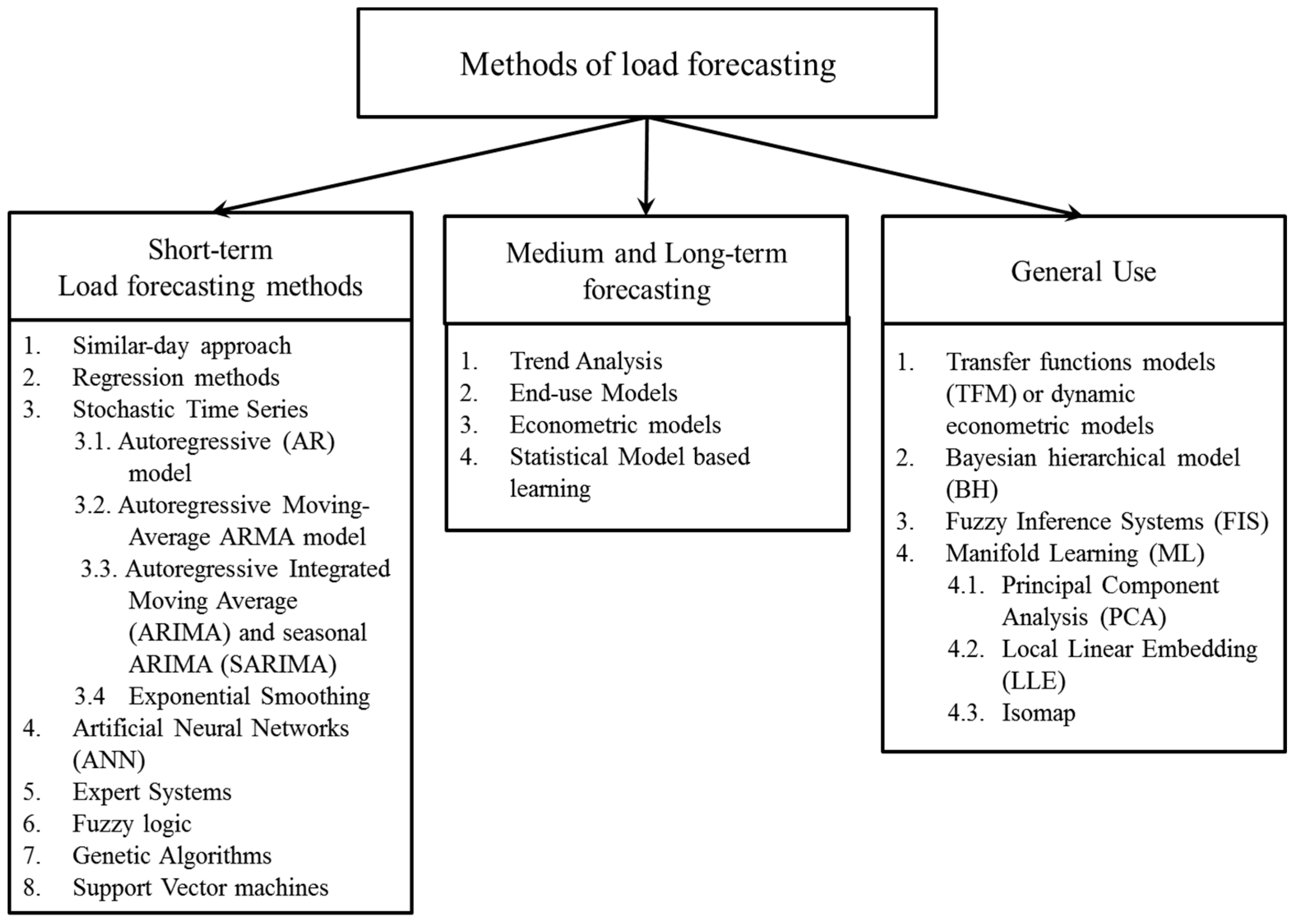
Figure 1 shows the spectrum of all methods categorized according to their short-term and medium to long-term usage, based on a literature review by the authors of this work. Other authors categorize the methods in two groups: classical mathematical statistical and artificial intelligence.
In order for this work to be as self-contained as possible with respect to the references we have decided to provide a short description of the most widely used methods in Figure 1. Further survey and review papers are provided for example in Heiko et al. [18], Kyriakides and Polycarpou) [19], Feinberg and Genethliou [20], Tzafestas and Tzafesta [21] and Hippert et al. [5] and a very recent one by Martinez-Alvarez et al. [22]. The group of models on the right part of Figure 1 contains new forecasting approaches that cannot be classified into any of the other two groups [
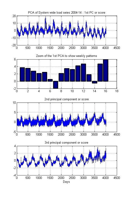
22]. A description of manifold learning Principal Component Analysis (PCA) technique is given in Section 4.3 and Section 5.2 below. Basic definitions of statistical tests and a short description of ETS models are given in Appendices A and B respectively while in Appendix C methods for Support Vector Machine (SVM) and ANN are also described.
Trend analysis uses historical values of electricity load and projects them into the future. The advantage of this method is that it generates only one result, future load, but provides no information on why the load evolves the way it does. The end-use method estimates electricity load, directly, by using records on end use and end users, like appliances, the customer usage profile, their age, type and sizes of buildings, etc. Therefore, end-use models explain electricity load as a function of how many appliances are in the market (Gellings [23]).
Combining economic theory and statistical analysis, the econometric models have become very important tools in forecasting load, by regressing various factors that influence consumption on load (the response variable). They provide detailed information on future levels of load, explain why future load increases and how electricity load is influenced by all the factors. The works of Genethliou and Feinberg [20], Fu Nguyen [24], and Li Yingying.; Niu Dongxiao [25], describe in depth both their theoretical structure and how they are applied in various markets. Feinberg et al., [26,27] developed statistical models that learn the load model parameters by using past data values. The models simplify the work in medium-term forecasting, enhance the accuracy of predictions and use a number of variables like the actual load, day of the week, hour of the day, weather data (temperature, humidity), etc.
The similar-day approach is based on searching historical data for days within one, two or three years with features that are similar to the day we want to forecast. The load of a similar day is taken as a forecast and we can also take into consideration similar characteristics of weather, day of the week and the date.
The technique that is the most widely used is regression analysis modeling and forecasting. We regress load on a number of factors like weather, day type, category of customers etc. Holidays, stochastic effects as average loads as well as exogenous variables as weather, are incorporated in this type of models. The works of Hyde et al. [28], Haida et al. [29], Ruzic et al. [30] and Charytoniuk et al. [31], provide various applications of this kind of models to load prediction. Engle et al. [32,33] applied a number of regression models for forecasting the next day peak value of load.
Stochastic time series load forecasting methods detect and explore internal structure in load series like autocorrelation, trend or seasonal variation. If someone assumes that the load is a linear combination of previous loads, then the autoregressive (AR) model can be fitted to load data. If the current value of the time series is expressed linearly in terms of its values at previous periods and in terms of previous values of white noise, then the ARMA model results. This model as well as the multiplicative or seasonal Autoregressive Integrated Moving Average (ARIMA, for non-stationary series), are the models that we will use in this work and are described in Section 4. Chen et al. [34] have applied an adaptive ARMA model for load prediction, where the resulting available prediction errors are used to update the model. This adaptive model outperformed typical ARMA models. Now, in case that the series is non-stationary, then a transformation is needed to make time series stationary. Differentiating the series is an appropriate form of transformation. If we just need to differentiate the data once, i.e., the series is integrated of order 1, the general form of ARIMA (p,1,q) where p and q are the number or AR and MA parameters in the model (see Section 4 for more details). Juberias et al. [35] have created a real time load forecasting ARIMA model, incorporating meteorological variables as predictors or explanatory variables.
References [36,37,38,39,40] refer to application of hybrid wavelet and ANN [36], or wavelet and Kalman filter [37] models to short-term load forecasting STLF, and a Kalman filter with a moving window weather and load model, for load forecasting is presented by Al-Hamadi et al. [38]. In the Greek electricity market Pappas et al. [39] applied an ARMA model to forecast electricity demand, while an ARIMA combined with a lifting scheme for STLF was used in [40].
Artificial Neural Networks (ANN) have been used widely in electricity load forecasting since 1990 (Peng et al. [41]). They are, in essence, non-linear models that have excellent non-linear curve fitting capabilities. For a survey of ANN models and their application in electricity load forecasting, see the works of Martinez-Alvarez et al. [22], Metaxiotis [42] and Czernichow et al. [43]. Bakirtzis et al. [44] developed an ANN based on short-term load forecasting model for the Public Power Corporation of Greece. They used a fully connected three-layer feed forward ANN and back propagation algorithm for training. Historical hourly load data, temperature and the day of the week, were the input variables. The model can forecast load profiles from one to seven days. Papalexopoulos et al. [45] developed and applied a multi-layered feed forward ANN for short-term system load forecasting. Season related inputs, weather related inputs and historical loads are the inputs to ANN. Advances in the field of artificial intelligence have resulted in the new technique of expert systems, a computer algorithm having the ability to “think”, “explain” and update its knowledge as new information comes in (e.g., new information extracted from an expert in load forecasting). Expert systems are frequently combined with other methods to form hybrid models (Dash et al. [46,47], Kim et al. [48], Mohamad et al. [49]).
References [50,51,52,53,54,55,56,57,58,59,60,61,62,63,64,65,66,67,68,69,70] cover the period 2000–2015 in which the work of Maier et al. [50] is one of the first ones related to ANN application in forecasting water resources, while during the same period we note also the creation of hybrid methods combining the strengths of various techniques that still remain popular until today. A combination of ANN and fuzzy logic approaches to predict electricity prices is presented in [51,52]. Similarly, Amjady [53] applied a feed-forward structure and three layers in the NN and a fuzzy logic model to the Spanish electricity price, outperforming an ARIMA model. Taylor [54] tested six models of various combinations (ARIMA, Exponential Smoothing, ANN, PCA and typical regression) for forecasting the demand in England and Wales. Typical applications of ANN on STLF are also presented in [55,56,57,58]. The book of Zurada [59] also serves as a good introduction to ANN. A wrapper method for feature selection in ANN was introduced by Xiao et al. [60] and Neupane et al. [61], a method also adopted by Kang et al. [62]. A Gray model ANN and a correlation based feature selection with ANN are given in [63,64]. The Extreme Learning Machine (ELM), a feed-forward NN was used in the works [65,66] and a genetic algorithm, GA, and improved BP-ANN was used in [67]. Cecati et al. [68] developed a “super-hybrid” model, consisting of Support Vector Regression (SVR), ELM, decay Radial Basis function RBF-NN, and second order and error correction, to forecast the load in New England (USA). A wavelet transform combined with and artificial bee colony algorithm and ELM approach was also used by Li et al. [69] for load prediction in New England. Jin et al. [70] applied Self Organizing Maps (SOM), a method used initially in discovering patterns in data to group the data in an initial stage, and then used ANN with an improved forecasting performance. One of the most recent and powerful methods is SVM, originated in Vapnik’s (Vane [71]) statistical learning theory (see also Cortes and Vapnik [72], and Vapnik [73,74]). SVM perform a nonlinear (kernel functions) mapping of the time series into a high dimensional (feature) space (a process which is the opposite of the ANN process). Chen et al. [75] provides an updated list of SVM and its extensions applied to load forecasting. SVM use some linear functions to create linear decision boundaries in the new space. SVM have been applied in load forecasting in different ways as in Mohandas [76], and Li and Fang [77], who blend wavelet and SVM methods.
References [76,77,78,79,80,81,82,83,84,85,86,87,88,89,90,91,92,93,94] on SVM and its various variations-extensions for performance improvement cover the period 2003–2016. Traditional SVM has some shortcomings, for example SVM cannot determine the input variables effectively and reasonably and it is characterized by slow convergence speed and poor forecasting results. Suykens and Vandewalle [78] proposed the least square support vector machine (LSSVM), as an improved SVM model. Hong [79] analyzed the suitability of SVM to forecast the electric load for the Taiwanese market, as Guo et al. [80] did for the Chinese market. To capture better the spikes in prices, Zhao et al. [81] adopted a data mining framework based on both SVM and probability classifiers. In order to improve the forecasting quality and reduce the convergence time, Wang et al. [82] combined rough sets techniques (RS) on the data and then used a hybrid model formed by SVM and simulated annealing algorithms (SAA). A combination of Particle Swarm Optimization (PSO) and data mining methods in a SVM was used by Qiu [83] with improved forecasting results. In general, various optimization algorithms are extensively used in LSSVM to improve its searching performance, such as Fruit Fly Optimization (FFO) [85,88], Particle Swarm Optimization (PSO) [93], and Global Harmony Search Algorithm [75].
The most recent developments on load forecasting are reviewed by Hong and Fan [95]. An interesting big data approach on load forecasting is examined by Wang [96], while Weron’s recent work is mostly focused on improving load forecast accuracy combining sister forecasts [97]. New methods on machine learning are covered in [98,99]. A regional case study is performed by Saraereh [100] using spatial techniques. Kim and Kim examine the error measurements for intermittent forecasts [101].
The structure of this paper is as follows: Section 2 includes a short description of the Greek electricity market with emphasis on the dynamic evolution of load during the 2004–2014 period. In Section 3 we quote the load series data performing all tests which are required for further processing by our models (stationarity tests, unit-root tests, etc.). Section 4 is the suggested methodology; it encompasses the mathematical formulation of the proposed models (SARIMAX, Exponential Smoothing and PC Regression analysis). 
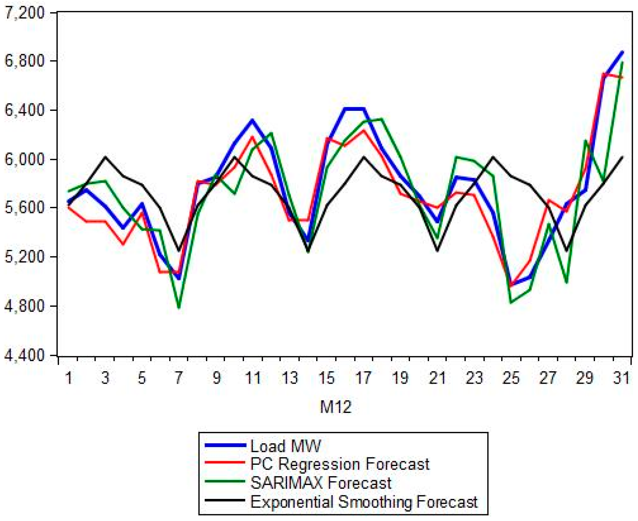
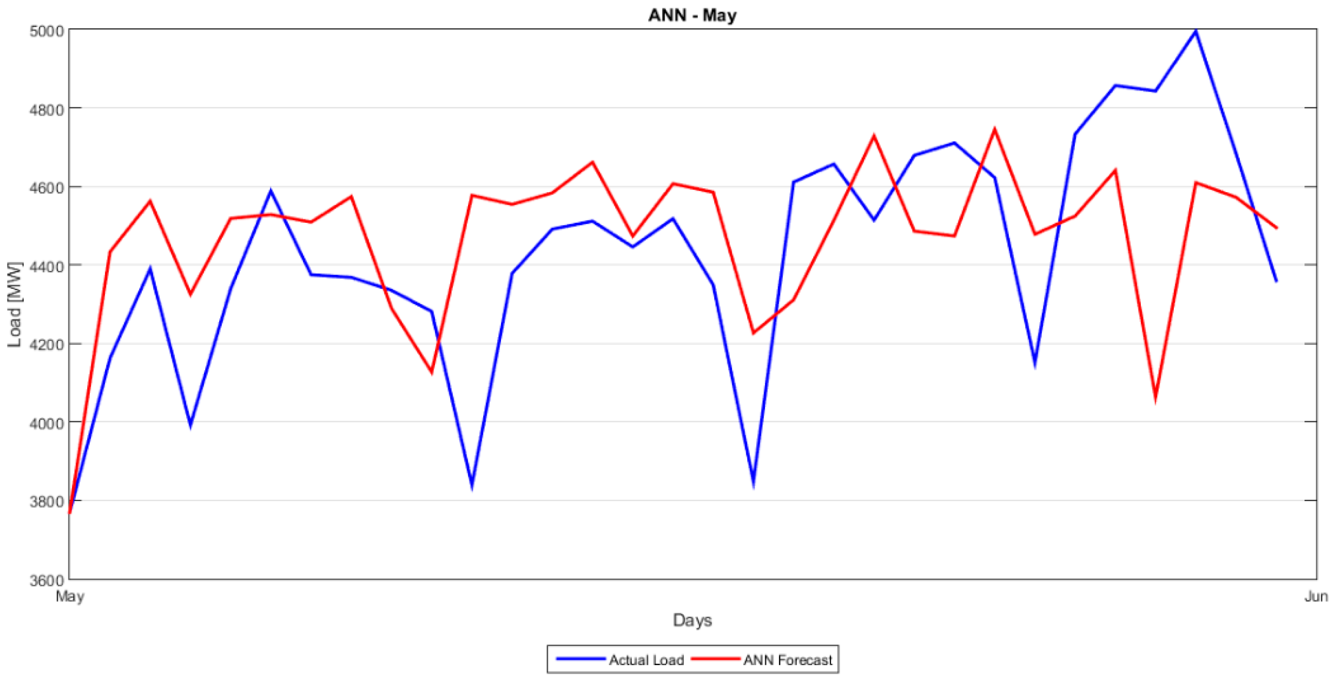
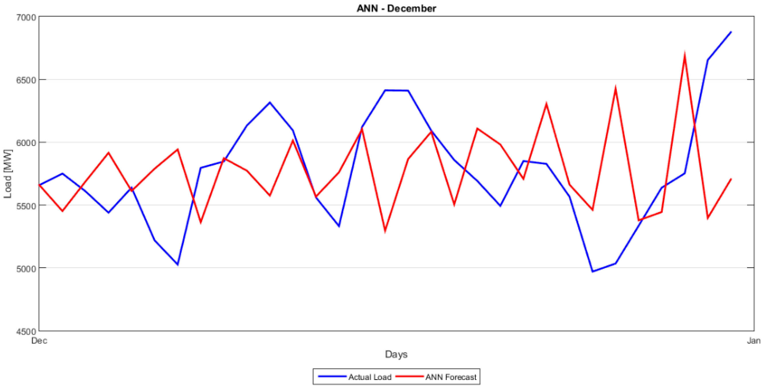
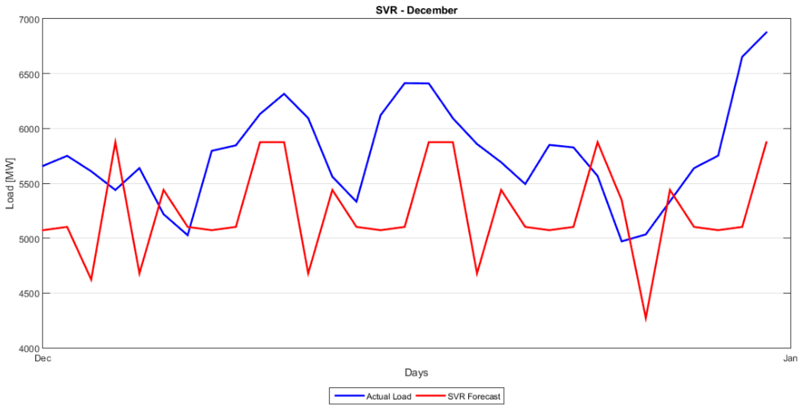
Section 5 presents the comparison between the proposed hybrid model and the classical forecasting methods as well as the more recent ANN and SVM approaches. A number of forecasting quality measures Mean Absolute Percentage Error (MAPE), Root Mean Squared Error (RMSE), etc. are evaluated and strengths and weaknesses of each model are noted. Section 6 (Conclusions) summarizes and proposes the next steps. A short description of the ANN and SVM methods is given in Appendix C.

2. Greek Electricity Market

A Short Description of the Greek Electricity Market

Greece’s liberalized electricity market was established according to the European Directive 96/92/EC and consists of two separate markets/mechanisms:
(1)
the Wholesale Energy and Ancillary Services Market;
(2)
The Capacity Assurance Mechanism.
The wholesale electricity market is a day ahead mandatory pool which is subject to inter-zonal transmission constraints, unit technical constraints and reserve requirements. More specifically, based on forecasted demand, generators’ offers, suppliers’ bids, power stations’ availabilities, unpriced or must-run production (e.g., hydro power mandatory generation, cogeneration and RES outputs), schedules for interconnection as well as a number of transmission system’s and power station’s technical constraints, an optimization process is followed in order to dispatch the power plant with the lower cost, both for energy and ancillary services. In this pool, market “agents” participating in the Energy component of the day-ahead (DA) market submit offers (bids) on a daily basis. The bids are in the form of a 10-step stepwise increasing (decreasing) function of pairs of prices (€/MWh) and quantities (MWh) for each of the 24 h period of the next day. A single price and quantity pair for each category of reserve energy (primary, secondary and tertiary) is also submitted by generators. Deadline for offer submission is at 12.00 pm (“gate” closure time).
The Operator of Electricity Market in Greece (LAGIE) [102] is responsible for the solution of the so-called day ahead (optimization) problem. This problem is formulated as a security constrained unit commitment problem, and its solution is considered to be the optimum state of the system at which the social welfare is maximized for all 24 h of the next day simultaneously. This is possible through matching the energy to be absorbed with the energy injected into the system, i.e., matching supply and demand (according to each unit’s separate offers). In the abovementioned optimization problem besides the objective function there are also a number of constraints. These are the transmission system constraints the technical constraints of the generating units and the energy reserves requirements. The DA solution, therefore, determines the way of operation of each unit for each hour (dispatch period) of the dispatch day as well as the clearing price of the DA market’s components (energy and reserves).
The ultimate result of the DA solution is the determination of the System Marginal Price (SMP, which is actually the hourly clearing price). At this price load representatives buy the absorbed energy for their customers while generators are paid for their energy injected into the system. The Real-Time Dispatch (RTD) mechanism refers to adjusting the day-ahead schedule taking into consideration data regarding availability and demand as well as security constraints. The dispatch scheduling (DS) is used in time period between day-ahead scheduling (DAS) and RTD where the producers have the right to change their declarations whenever a problem has been occurred regarding the availability of their units. Any deviations from the day-ahead schedule are managed via the imbalances settlement (IS) operation of the market. During the IS stage an Ex-Post Imbalance Price (EXPIP) is produced after the dispatch day which is based on the actual demand, unit availability and RES production. The capacity assurance mechanism is a procedure where each load representative is assigned a capacity adequacy obligation and each producer issues capacity availability tickets for its capacity. Actually this mechanism is facing any adequacies in capacity and is in place for the partial recovery of capital costs.
The most expensive unit dispatched determines the uniform pricing in the day-ahead market. In case of congestion problems and as a motive for driving new capacity investment, zonal pricing is a solution, but at the moment this approach has not been activated. Physical delivery transactions are bounded within the pool although market agents may be entering into bilateral financial contracts that are not currently in existence. The offers of the generators are capped by an upper price level of 150 €/MWh.

3. Data Description and Preparation

This section is devoted to the description and preprocessing of the data available. The main time series we focus on is the system load demand in the Greek electricity market. This is defined as the system’s net load; more specifically the system’s net load is calculated as the sum demanded by the system (total generation including all types of generation units, plus system losses, plus the net difference of imports & exports, minus the internal consumption of the generating units). In this article we use the terms system load and load interchangeably.
The raw data are provided by Independent Power Transmission Operator (IPTO or ADMIE) (http://www.admie.gr) and include the hourly and daily average load, for the 10 year period from 1 January 2004 to 31 December 2014, as well as average external temperature in Greece, for the same time period.
In this work, we aim to capture the effect of seasonal events on the evolution of the load demand [4,103]. For this reason and as bibliography suggests, we also include as exogenous variables three indicator vectors that use Boolean logic notation to point states like working days, weekend and holidays. The study is conducted on the Greek electricity market, therefore we consider the Greek holidays (Christmas, Orthodox Easter, Greek national holidays). The abovementioned vectors and the temperature are imported as exogenous variables to the SARIMA model for building our final SARIMAX model (see Section 4).
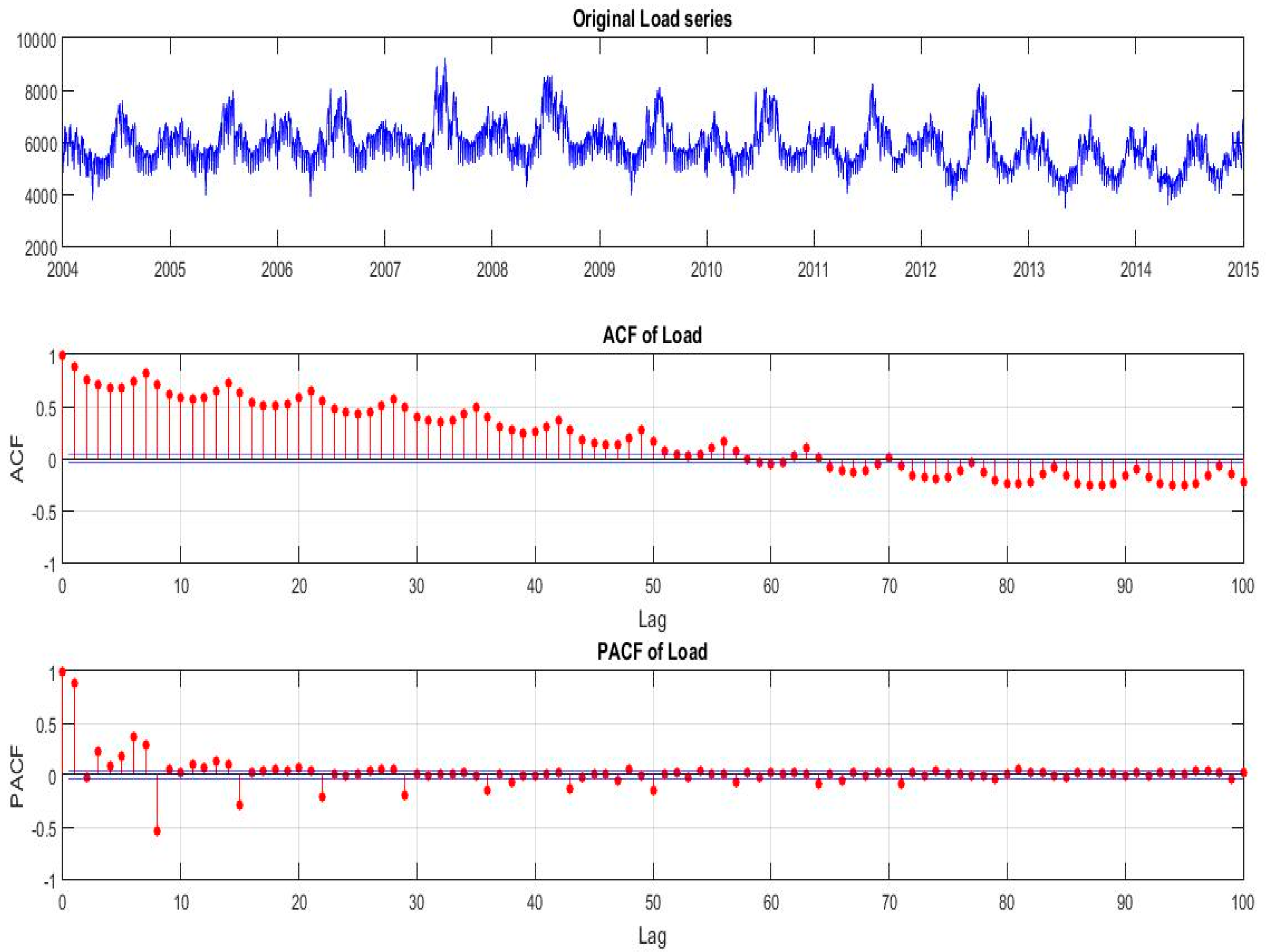
Figure 2 shows the evolution of load demand in Greece for the time period 2004–2014. We also plot the Autocorrelation Function (ACF) and Partial Autocorrelation Function (PACF) of the load for the period 2004–2014. From this plot we observe strong, persistent 7-day dependence and that both the ACF and PACF decay slowly, indicating a strong autocorrelated or serially correlated time series. This is a strong indication of seasonality in our load series and also an implication of non-stationarity. The PACF also shows the seasonality with spikes at lags 8, 15, 22 and so on. Table 1 provides the summary or descriptive statistics of the load and temperature time series.
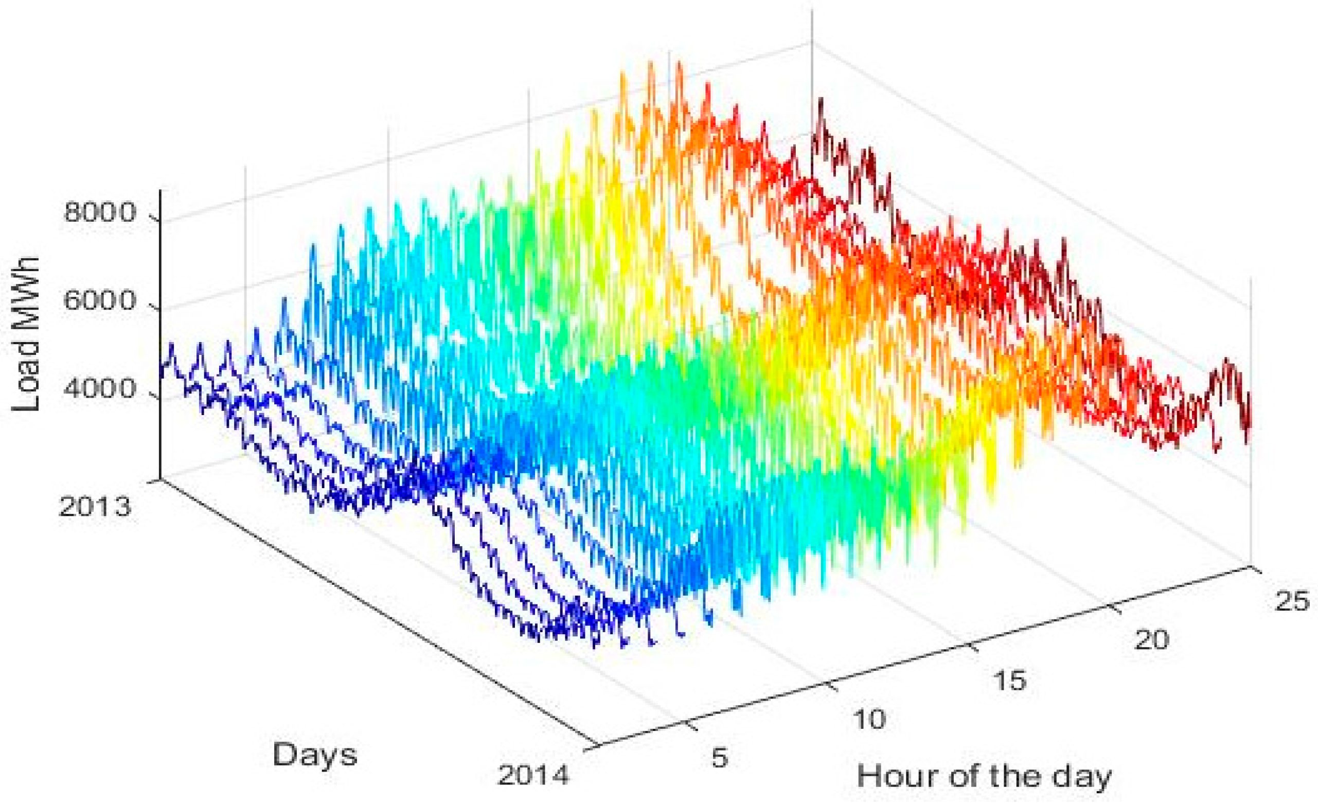
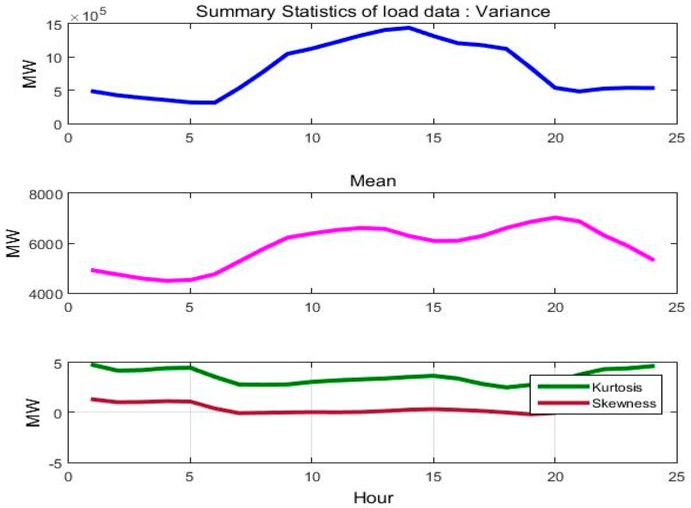
Figure 3 depicts the evolution of load for each hour of the day for the year 2013, while in Figure 4 we show the fluctuation of the mean, variance, kyrtosis and skewness of load for each hour of the day and for the period 2004–2014.
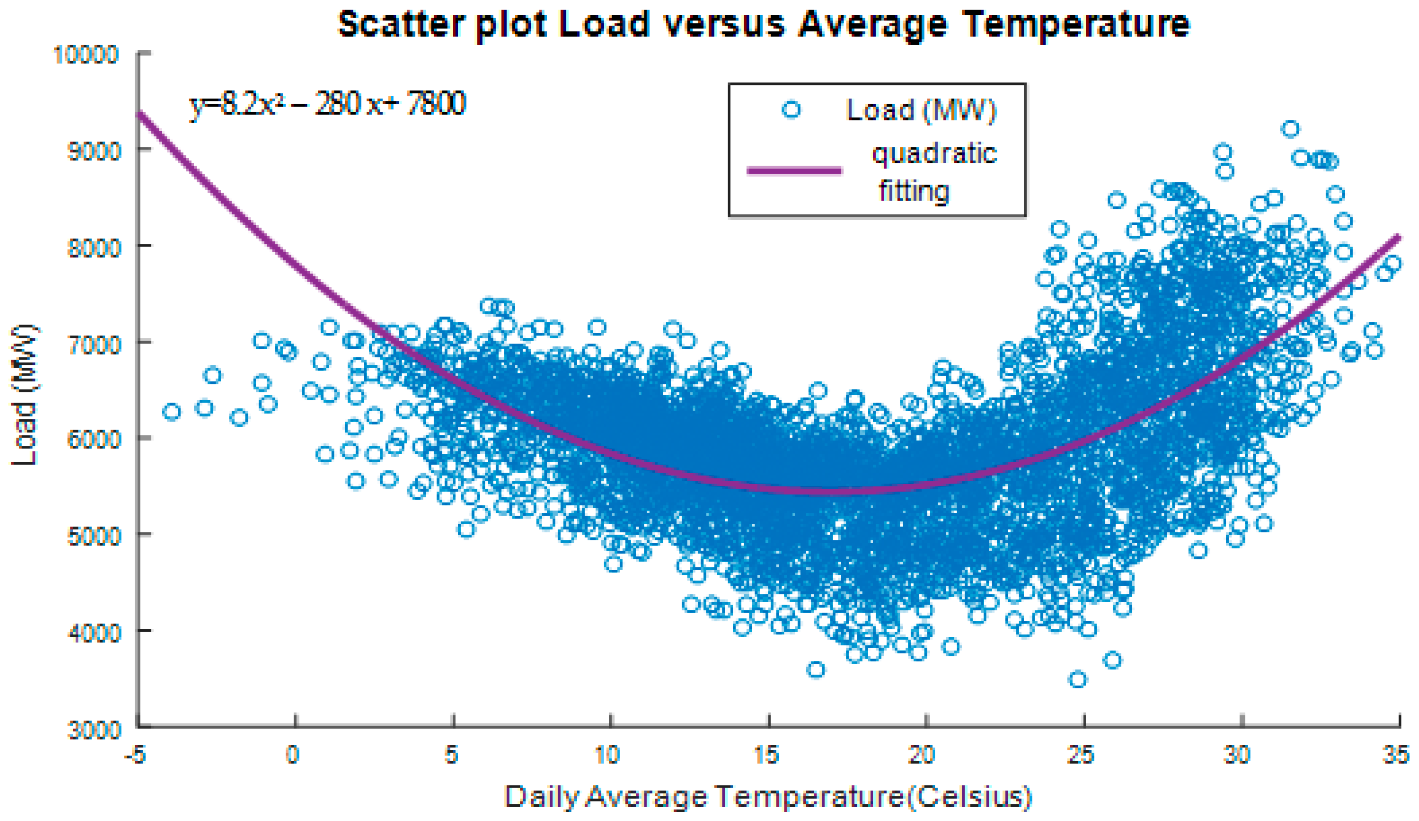
The variation of load with average daily temperature is depicted in Figure 5.
The graph shows a parabolic shape indicating increased consumption at high and low temperatures [33]. It suggests also that forecasting future load (demand), requires the knowledge of load growth profile, relative to a certain reference i.e., the current year. The polynomial function of load versus temperature shown on the graph seems a reasonable approximation for load forecasting. Due to quadratic and strong correlation between temperature and load, we have included temperature as an exogenous—explanatory variable in the modeling in order to enhance model’s predictive power. More specifically, we have considered the temperature deviation from comfortable living conditions temperature in Athens, for the current and previous day T A t h 2 ( t ) ,   T A t h 2 ( t 1 ) respectively (Tsekouras [104]):
T d e v i a t i o n 2 = { ( T c T ) 2 , T < T c 0 , T c < T < ( T T h ) 2 , T h < T T h
where Tc = 18 °C, Th = 25 °C. This expression for T d e v i a t i o n capture the nonlinear (parabolic) relation of temperature and system load shown in Figure 5.
The same plot is expected if instead of the daily average temperature we use daily maximum or minimum temperature. 
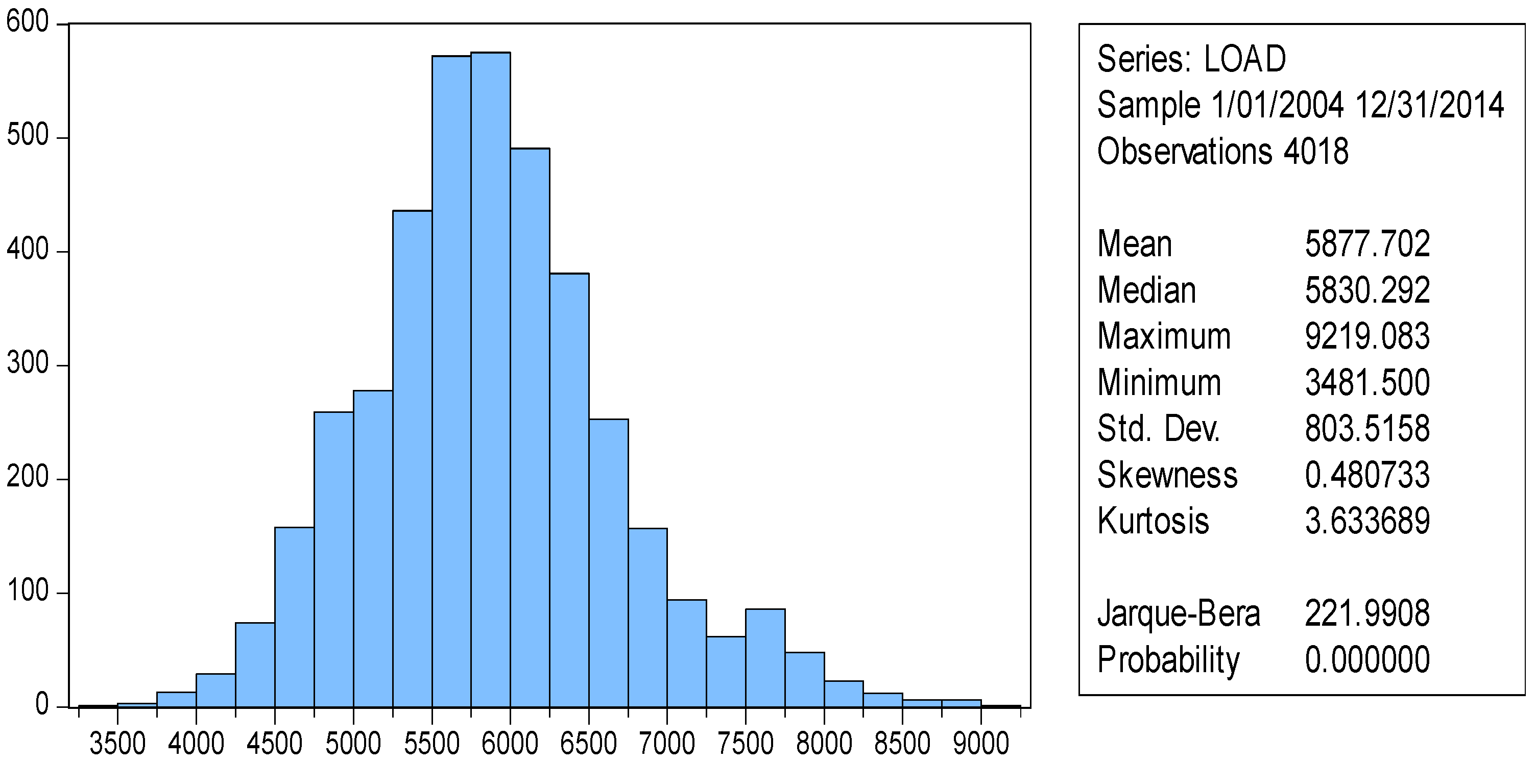
Figure 6 gives the histogram of the load as well as its summary statistics.
Before proceeding to formulate a model, we apply various statistical tests in order to examine some core properties of our data, namely stationarity, normality, serial correlation, etc. The Jarque and Bera (JB) algorithm [105] assumes the null hypothesis that the sample load series has a normal distribution. The test as we see rejected the null hypothesis at the 1% significance level, as it is shown in the analysis (p = 0.000, JB Stat significant). From the descriptive statistics of the above figure the positive skewness and kurtosis indicate that load distribution has an asymmetric distribution with a longer tail on the right side, fat right tail. Thus load distribution is clearly non-normally distributed as it is indicated by its skewness (different but still close to zero), and excess kurtosis (>3) since normal distribution has kurtosis almost equal to three (3). That means that our data need to be transformed in such way in order to have a distribution as close to normal as possible.
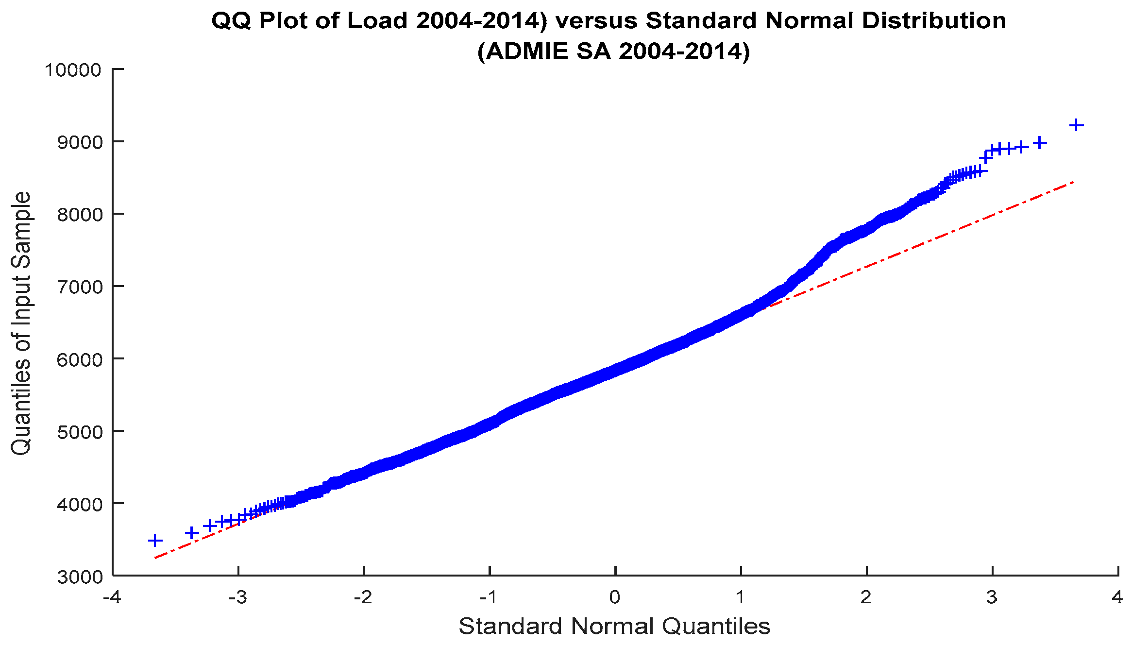
The deviation of load distribution from normality is also apparent in the Q-Q plot, Figure 7. We see that the empirical quantiles (blue curve) versus the quantiles of the normal distribution (red line) do not coincide, even slightly and exhibit extreme right tails:
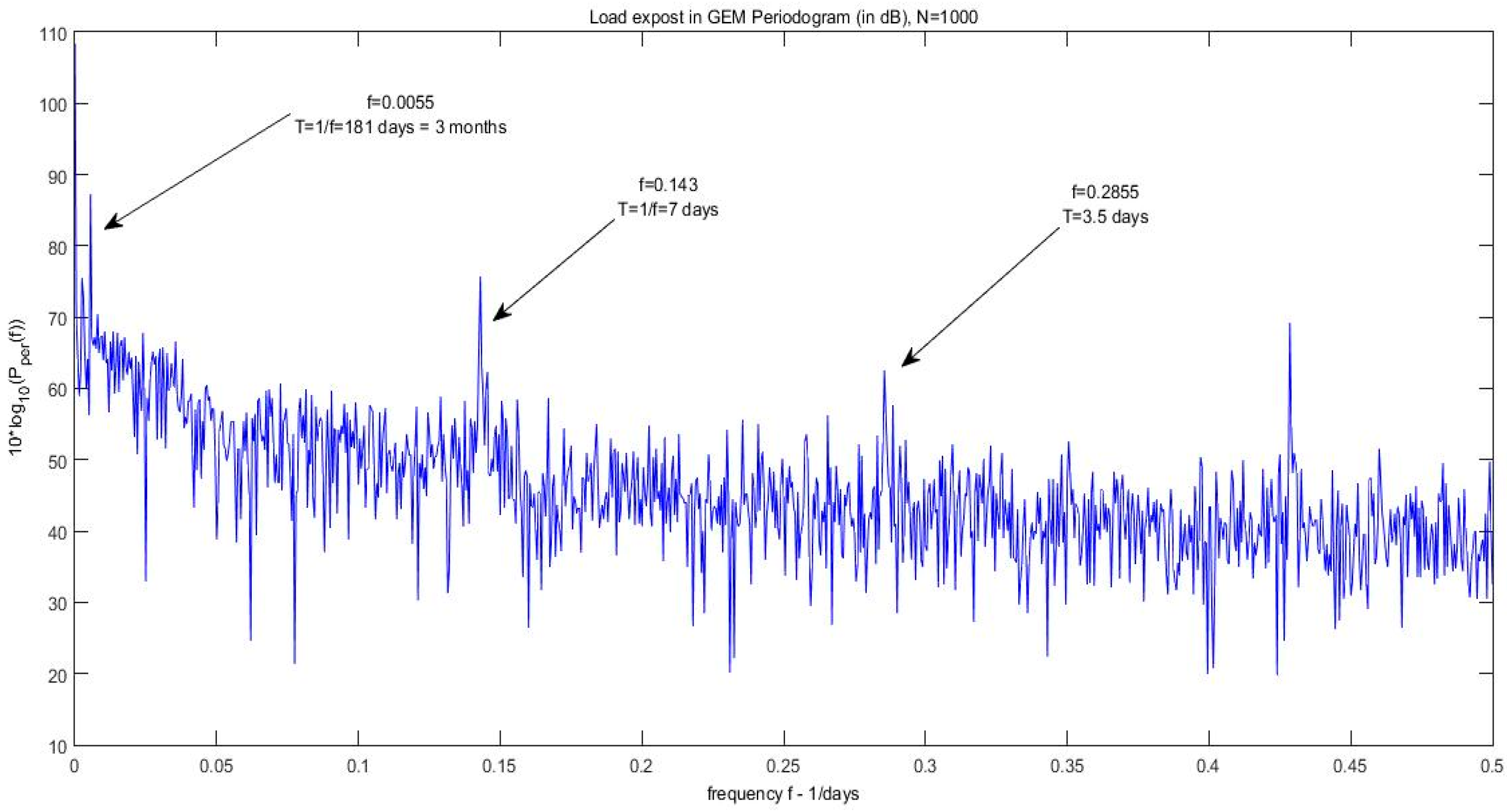
In this section we also identify the cyclical patterns of load for the period 2004 to 2014. This can be done by decomposing our signals which contain cyclical components in its sinusoidal functions, expressed in terms of frequency i.e., cycles per unit time, symbolized by ω. The period, as we know, is the reciprocal of ω i.e., T = 1/ω. Since our signal is expressed in daily terms, a weekly cycle is obviously 1/0.4128 = 7 days or 1/52.14 = 0.0192 years expressed annually. A typical tool for revealing the harmonics or spectral components is the periodogram. Let our set of signal measurements or the load time series is {xi, i = 1,…n}, then the periodogram is given as follows:
I n ( ω k ) = 1 n   | t = 1 n x t e x p i ( t 1 ) ω k | 2
where ω k = 2 π ( k / n ) are the Fourier frequencies, given in radians per unit time. In Figure 8 the periodogram of daily average system load is shown, for the same period as before. Obviously the signal exhibits the same periods and its harmonics as described above. The periodic harmonics identified in this graph correspond to 7-day period (peak), 3.5-day and 2.33-day (bottom part) which in turn correspond to frequencies ωk = 0.1428, 0.285 and 0.428 respectively (upper part of the figure). The existence of harmonics i.e., multiples of the 7-day periodic frequency reveal that the data is not purely sinusoidal.
We treat load as a stochastic process and before proceeding further in our analysis, it is necessary to ensure that conditions of stability and stationarity are satisfied. For this purpose, we will utilize the necessary tests proposed by bibliography [106], Augmented-Dickey-Fuller (ADF) [107] test for examination of the unit-root hypothesis and Kwiatkowski-Phillips-Schmidt-Shin (KPSS) [108] test for stationarity. Applying the ADF test we acquire the information that the series is stable; therefore null hypothesis is rejected. Additionally performing the KPSS test to the load series, we also obtain that the null hypothesis is rejected hence our time series is non-stationary. Even after applying 1st difference, although this forces the time series to become stationary, as the KPSS test applied on the 1st difference also confirms, the ACF and PACF still suggest that a seasonality pattern is present, at every 7 lags. Therefore, we will proceed and filter our data through with a 1st and 7th order differencing filter. The above tests ensure that the stability and stationarity requirements are met [8]. The aforementioned preliminary tests, as shown in Table 2, indicate that our time series has to be differenced before we fit it in a regressive model.
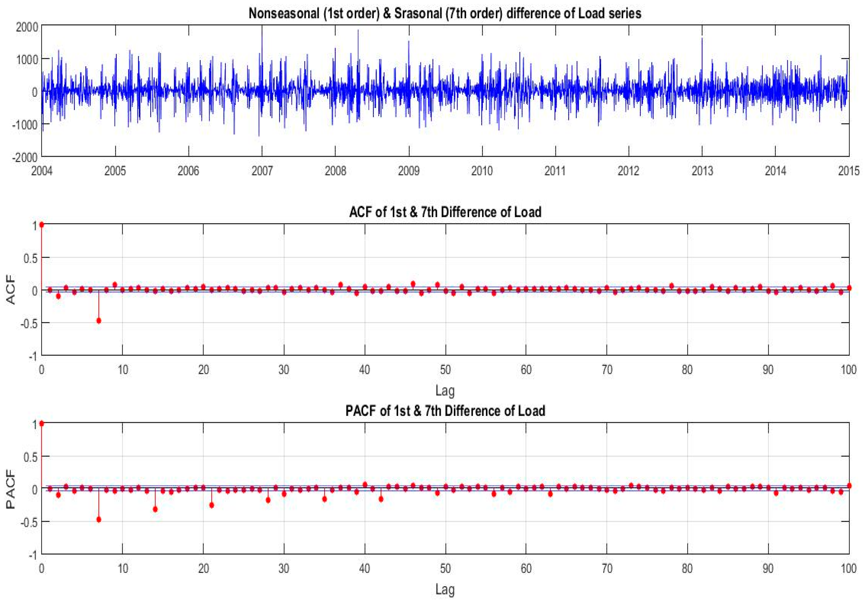
The slowly decaying positive ACF in Figure 2, after 1st differencing, becomes a slowly decaying but still an oscillatory behavior with 7 lags period, a fact suggesting the need to fit a seasonal (multiplicative) ARMA model to our data. The damping of this oscillation is faster as the ACF value is away for the value of 1. Therefore, in order to capture the 7 lags-period seasonality in load time series, we must also apply, in addition to 1st difference operator (1−B), the operator (1−B7), on x t (load). The needed transformed series is given by:
( 1 B ) ( 1 B 7 ) x t
i.e., the nonseasonal first difference times the seasonal (of period 7 days) difference times Load, where B s x t = x t s , the lag operator. In Figure 9 we show the ACF and PACF of the transformed series.

4. Suggested Methodology—Mathematical Formulation

4.1. The Seasonal ARIMA and ARIMAX Models

The seasonal (or multiplicative) ARIMA model (SARIMA) is an extension of the Autoregressive Integrated Moving Average (ARIMA) [8,9] model, when the series contains both seasonal and non-seasonal behavior, as our time series load does. This behavior of load makes the typical ARIMA model inefficient to be used. This is because it may not be able to capture the behavior along the seasonal part of the load series and therefore mislead to a wrong selection for non-seasonal component.
Let d and D are nonnegative integers, the series { x t } is a seasonal ARIMA (p, d, q) (P, D, Q)S process with seasonality or period s if the differenced series:
y t = ( 1 B ) d ( 1 B s ) D x t
is a casual ARMA process (Brockwell and Davis, [9]), defined by:
φ p ( B ) Φ P ( Β s ) y t = θ q ( B ) Θ Q ( B s ) ε t   ,   ε t   ~ W N ( 0 , σ 2 )
where B is the difference or lag operator, defined in Section 3, and φ(x), Φ(x), θ(x) and Θ(x) polynomials defines as follows:
φ p ( x ) = 1 φ 1 x φ p x p ,   Φ P ( x ) = 1 Φ 1 x Φ P x P
θ q ( x ) = 1 + θ 1 x + + θ q x q   a n d   Θ Q ( x ) = 1 + Θ 1 x + + Θ Q x Q
In the ARIMA form (p, d, q) (P, D, Q)S the term (p, d, q) is the non-seasonal and P, D, Q)S is the seasonal part. We note here that the process y t is casual if and only if φ(x) ≠ 0 and Φ(x) = 0 for | x | 1 while in applications d is rarely more than 1, D = 1 and P and Q are typically less than 3 (Brockwell & Davis, 1996) [9]. Also, if the fitted model is appropriate, the rescaled residuals should have properties similar to those of a white noise ε t driving the ARMA process. All the diagnostic tests that follow, on the residuals, after fitting the model, are based on the expected properties of residuals under the assumption that the fitted model is correct and that { ε t } ~ W N ( 0 , σ 2 ) .
In order to incorporate eXogenous variables in the SARIMA model, to obtain a SARIMAX model the previous model is modified as follows:
φ p ( B ) Φ P ( Β s ) y t = c + β X t + θ q ( B ) Θ Q ( B s ) ε t
where y t as previously is the univariate response series, in our case load X t is the row t of X, which is the matrix of predictors or explanatory variables, β is a vector with the regression coefficients corresponding to predictors, c is the regression model intercept, and ε t is a white noise innovation process. The φ p ,   Φ P ,   θ q and Θ Q are as previously defined i.e., the lag operator polynomials, seasonal and nonseasonal:
φ p ( B ) n o n s e a s o n a l   A R Φ P ( Β s ) s e a s o n a l A R   ( S A R ) ( 1 B ) d n o n s e a s o n a l i n t e g r a t i o n ( 1 B s ) D s e a s o n a l   i n t e g r a t i o n x t =
= c i n t e r c e p t + β X t e x o g e n o u s   v a r i a b l e s + θ q ( B ) n o n s e a s o n a l   M A Θ Q ( B s ) s e a s o n a l   M A   ( S M A ) ε t   ,   ε t   ~ W N ( 0 , σ 2 )

4.2. A Short Description of Exponential Smoothing (ES) and Error-Trend-Seasonal (ETS) Forecasting Methods

The exponential smoothing approaches date back to the 1950s. However, procedures for model selection were not developed until relatively during our days. All exponential smoothing methods (including non-linear methods) have been shown to be optimal forecasts from innovations state space models (Hyndman et al. [109,110]). Pegels [111] was the first to make a taxonomy of the exponential smoothing methods. Hyndman et al. [109] modified the work of Gardner [112] who had previously extended the work of Pegels’ [111] classification table. Finally, Taylor [113] provided the following Table 3 with all fifteen methods of exponential smoothing.
However, a subset of these methods is better known with other names. For instance, the well-known simple exponential smoothing (or SES) method corresponds to cell (N, N). Similarly, cell (A, N) is Holt’s linear method, and the damped trend method is given by cell (Ad, N). Also, the additive Holt-Winters’ method is given by cell (A, A) while and the multiplicative Holt-Winters’ method is given by cell (A, M). As it is described in Weron [114] and Taylor [115], exponential smoothing is the traditional model used in forecasting load data series. Due to its satisfactory results it has been adopted by lots of utilities. However, it is pointed out in the above paper that seasonal multiplicative smoothing, SMS, or a variant of it Holt-Winter’s SMS are very useful in capturing the seasonal (periodicity) behavior. Centra [116], has applied a Holt-Winter’s SMS model to forecast hourly electricity load.
The given time series Y may be decomposed into a trend (T), seasonal (S) and error (E) components. The trend reflects the long-term movement of Y, the seasonal corresponds to a pattern with known periodicity and the error is the uncertain, unpredictable constituent of the series.
In a purely additive model we have: Y = T + S + E or Y = S + T, while in a pure multiplicative model: Y = T·S·E or Y = T·E. Hybrid models are: Y = (T·S) + E or Y = (T + S)(1 + E).
Let now the forecasted trend T h periods out, by these models, be decomposed into a level term (l) and a growth term (b) in a number of ways. Let also 0 < φ < 1 be the damping parameter. The five different trend types, according to different assumptions about the growth term.
Additive T h = l + b · h
Additive damped T h = l + b · φ h
Multiplicative T h = l · b h
Multiplicative damped T h = l · b φ
None T h = l
where φ h s = 1 h φ s .
Let also s represent the included seasonal terms, we can define the general p-dimensional state vector:
x t ( l t , b t , s t , s t 1 , , s t m )
A nonlinear dynamic model representation of the ES equations using state space model with a common error part (Ord [117]):
y t = h ( x t 1 , θ ) + k ( x t 1 , θ ) ε t
x t = f ( x t 1 , θ ) + g ( x t 1 , θ ) ε t
where h, k continuous scalar functions, f and g continuous functions with continuous derivatives, p P and ε t ~ i i d   W N ( 0 , σ 2 ) , independent past realizations of y and x. θ is a parameter set. Intuitively, y t reflects the way the various state variables ( l t 1 , b t 1 , s t m ) are combined to express y t ^ = h ( x t 1 , θ ) and ε t . With additive errors we have k ≡ 1, so:
y t = h ( x t 1 , θ ) + ε t
with multiplicative errors, k h , so:
y t = h ( x t 1 , θ ) ( 1 + ε t )
For the ETS models we applied in this work, we consider the updating smoothing equations as being weighted average of a term depending on the current prediction error (and prior states), and one depending on the prior states. The general form of the resulting state equations is:
l t = a P ( x t 1 , ε t ) + ( 1 a ) Q ( x t 1 )
b t =   β R ( x t 1 , ε t ) + ( 1 β ) φ 1 b t 1 φ 2
s t   = γ T ( x t 1 , ε t ) + ( 1 γ ) s t m
where P t P ( x t 1 , ε t ) R t and T t are functions of the forecasting error and lagged states and Q t = Q ( x t 1 ) is a function of the lagged states. φ 1 ,   φ 2 are the damping parameters for linear trend and multiplicative trend models respectively (they are = 1, in the absence of damping). The exact form of (10–12) depends on the specific ETS specifications. Hydman et al. [118], list all the 30 possible specifications (see Tables 2.2, 2.3, pages 21–22 in this reference).

Simple Exponential Smoothing (A,N,N)

By inserting x t = l t and h ( x t 1 , θ ) = l t 1   ,   P t = l t 1 + ε t and Q t = l t 1 in Equations (8) and (9) the ETS representation of this (A,N,N) model, in the form of (10–12) is:
y t = l t 1 + ε t
l t = l t 1 + a ε t
Similarly, the ETS expressions for the models Holt’s Method with multiplicative Errors (M,A,N) and Holt-Winters method with multiplicative errors and seasonal (M,A,M), and fully multiplicative method with damping (M,Md,M), are given in the Appendix B.

4.3. Manifold Learning and Principal Component Analysis in Electricity Markets

The Need for a Low Dimensional Presentation of Electricity Load Series

The work needed to analytically model the dynamic evolution of a load curve is daunting since the load series is a relatively “high-dimensional” quality. Each load value at a point in time (say an each hour of the day) on the load curve essentially contains one dimension of uncertainty, due to the concurrent influence of both fundamental and random disturbance factors. Therefore, it seems natural to reduce the dimensionality of modeling a load curve and identify the major random factors that affect its dynamics.
Principal Component Analysis (PCA) is a linear manifold learning technique, mainly suited for extracting the linear factors of a data or time series. In the case of hourly day-ahead electricity load series, the assumption that a low-dimensional structure capturing the longest amount of randomness in the load dynamics seems to be reasonable. Furthermore, while the electricity delivered in the next 24 h corresponds to different commodities, the different 24 prices all result from equilibrating the fundamental supply and demand (load). The load demand and supply conditions in all 24 h suggests for a possible linear or non-linear representation of both the 24-dimensional load and price series in a manifold or space of lower dimension.
In this work we apply the PCA method of manifold learning, in order to analyze the “hidden” structures and features of our high-dimensional load data. Other more advanced method in manifold learning, like Locally Linear Embedding (LLE) or Isometric Feature Mapping (ISOMAP), to capture intrinsic non-linear characteristics in load data, could be used, but this is left for our next work.
As it is observed, the load demand series is highly correlated, hinting that the high dimension of the original data can be reduced to a minimum realization state space. To achieve the necessary dimension reduction we seek data structures of the fundamental dimension hidden in the original observations. For this reason we apply PCA (Jolliffe, [119]) and seek data sets that maintain the variance of the initial series, allowing only an insignificant portion of the given information to be lost. The PCA provides a new data set of drastically reduced dimension, to which a regression model is applied. This strategy provides a reliable forecasting method, with variables reduced to the minimum necessary dimension, allowing for faster calculations and reduced computational power.
In a multiple regression, one of main tasks is to determine the model input variables that affect the output variables significantly. The choice of input variables is generally based on a priori knowledge of casual variables, inspections of time series plots, and statistical analysis of potential inputs and outputs. PCA is a technique widely used for reducing the number of input variables when we have huge volume of information and we want to have a better interpretation of variables (Çamdevýren et al. [120], Manera et al. [121]). The PCA approach introduces a few combinations for model input in comparison with the trial and error process. Given a set of centered input vectors h 1 , h 2 , …, h m (i.e., hour 1 ( h 1 ) , hour 2 ( h 2 ) ,..., hour 24 ( h 24 ) ) and t = 1 m h t = 0 . Then the covariance matrix of vector is given by:
C = 1 l t = 1 l h t h t T
The principal components (PCs) are computed by solving the eigenvalue problem of covariance matrix C:
λ i u i = C u i   ,   i = 1 , 2 , , m ,
where λ i is one of the eigenvalues of C and u i is the corresponding eigenvector. Based on the estimated u i , the components of z t ( i ) are then calculated as the orthogonal transforms of h t :
z t ( i ) = u i T h t ,   i = 1 , 2 , , m .
The new components z t ( i ) are called principal components. By using only the first several eigenvectors sorted in descending order of the eigenvalues, the number of principal components in z t can be reduced, so PCA has the dimensional reduction characteristic. The principal components of PCA have the following properties: z t ( i ) are linear combinations of the original variables, uncorrelated and have sequentially maximum variances (Jolliffe [119]). The calculation variance contribution rate is:
V i = λ i i = 1 m λ i × 100 %
The cumulative variance contribution rate is:
V ( p ) = i 1 p V i
The number of the selected principal components is based on the cumulative variance contribution rate, which as a rule is over 85%–90%.
Table 4 gives the four (4) largest eigenvalues λ i or variance of the Covariance matrix C , the corresponding variance contribution rate (or % of variance explained) V i and the cumulative variance contribution. Figure 10 provides the patterns of the first four eigenvectors.
We see that the first principal component explains the largest part of the total variation (83.82% on average), which represents the system load pattern within a typical week. The second and third components (8.79% and 3.65%, respectively) capture some specific aspects of system load, basically daily effects and environmental factors.
Looking at the middle part of Figure 4, we observe that the mean average system load curve exhibits a significant difference in its pattern between night and day. In Figure 10 we show the four eigenvectors u i associated with the first four eigenvalues λ i ( i = 1 , , 4 ) .
The 24 coefficients associated with u 1 , mimic very closely the pattern of the average system load curve, confirming the explanatory power of this component. By observing the values of the first PC ( Z t ( 1 ) ) in Figure 11 (a zoom), they are positive and almost constant during the first part of the week, while reduced during Saturdays and finally negative during Sundays. This is actually the general shape of the aggregate system load daily pattern, i.e., more “active” during working days and “less” active on week-ends and holidays. These features are captured well by PC1. The differences in load values between working days and week-ends within each week, are captured by the coefficient of the second component u 2 . This component helps define the shape of the system load curve during working days.
The third component PC3 explains on average, as we already said, only a small proportion of the variance in system load and it probably accounts for the effects of weather conditions and environmental factors. The length of the day during winter is shorter so the electricity consumption for heating and lighting is very high during the late afternoon. On the contrary, consumption is lower in late afternoon in summer, due to the fact that daylight is intense and the mean temperature is not as high as in the middle of the day to justify a massive use of air conditioning.
We then perform a typical regression where the response variable is the daily average system load and predictors the first three PCs, following the same rationale as in [68]:
Y = l o a d = c 0 + c 1 z t ( 1 ) + c 2 z t ( 2 ) + c 3 z t ( 3 ) + ε t   ,   ε t ~ W N ( 0 , σ 2 )
As new information flows by (the set of new values of the system load for each hour of the new day), a new set of PCs is extracted from the updated covariance matrix C, and a new regression is performed.
Figure 12 shows the factor loading structure, the “projection” of the original matrix of data on the low dimensional manifold spanned by the three or four eigenvectors. It shows the loading of each variable h 1 ,…, h 24 (each hour in the day) on the 1st, 2nd, 3rd and 4th PC. PC1 explains the 83.83% of the total variability (variance) of the variables, while PC2 explains only the 8.79%, etc. We observe the coefficients of the loadings in Figure 12, while a 3D picture of the first four principal components or ‘scores’ is given in Figure 13. The distribution of points (dots) along the three individual axes (PC’s) of this 3D ‘manifold’ is very clear. The variances of the distribution of points on the axes correspond to the magnitude of the three largest eigenvalues of the covariance matrix. A piece of very interesting information results from comparing the profiles of structure of the first four eigenvectors in Figure 12 with the profiles of variance, mean and kurtosis of h 1 to h 24 , of Figure 4. The similarity of the profiles suggests that the four loadings provide information about the variance (corresponding to PC1), skewness (PC2), mean (PC3) and kurtosis (PC4) contained in our data set. The capacity of PCA to reproduce the “same” qualitative features of the original 24D manifold with a low dimensional (3D or 4D) manifold is clearly shown.

5. Proposed Load Forecasting Models and Comparison

5.1. Application of SARIMAX Model and Results

For the discussed load series (first difference of load), we extracted the best performing model following the Box-Jenkins methodology, from a huge set of 1521 possible models. The selected estimation sample includes observations starting from 1 January 2004 for each model, since we observed that shorter samples produce less efficient models.
Next we examine carefully the ACF and PACF of the filtered series in Figure 9. More specifically we observe the lags that are multiples of seven (s = 7) in order to determine the Q and P parameters from ACF and PACF, respectively. From the PACF we observe that lags at 7, 14, 21, 28, 35 and 42 are outside the bounds suggesting that P should be ranged between 1 and 6. Moreover, from the ACF we observe that the lag at 7 and possibly at 14 and 21 are outside the bounds suggesting Q = 1 to 3. The orders of p and q are then selected by observing the non-seasonal lags observed before lag 7, where we conclude at p = 1 to 4 (lags at 1 to 4) and q = 1 to 2. In other words a preliminary SARIMA model to start with, could have the following form:
SARIMAX   ( 1   to   4 ,   1 ,   1   to   2 ) ( 1   to   6 ,   1 ,   1   to   3 ) 7
We estimated all of the SARIMAX models developed in this work using the maximum likelihood standard procedure. The Schwartz Bayesian criterion or BIC and Akaike information criterion, AIC, were used to select the models with the requirements that all regression coefficients (see Table 5) were significant (at the 1% level). Table 6 provides the values of the above two criteria, which must be the minimum possible ones for a model to be a good candidate for selection.
The SARIMAX method involves the selection of the exogenous variables. Many research findings indicate that temperature is a crucial factor for load forecasting and more importantly, the deviation of temperature from the heating and cooling indices, 25 °C and 18 °C, respectively (Hor et al. [122], Tsekouras et al. [104]). In our case, as observed in Figure 5, there is a profound quadratic relation between temperature and the load curve. Thus, we conclude in a set of exogenous variables comprised of the deviation of temperature from the mentioned indices for the given day, and the deviation for the past two days, to account for the ‘social inertia’, a force that compels masses to react with a certain delay to events. Additionally, we take into consideration a couple of other social parameters that drive the demand of the load, working days and holidays.
The estimation output of the above SARIMAX model is given in the following Table 5. The estimation is based on a period of 10 years, 2004–2013. Table 5 shows the coefficient estimates all having the expected sign, the standard error, the t-statistics and the coefficient of determination R 2 . All coefficients are statistically significant at 1% level (p-values = 0.000).
Observing the fitted model we enhance our intuition on the relation between temperature and load. For example, the deviation of temperature to the heating index is weighted 7.569. Therefore, we expect for a working day with average temperature 30 °C that the load should increase roughly by 7.569 ( 25 30 ) 2 = 189.2   MW from its average value 5943.5 MW and it should equal 6132.7 MW. As it appears, given our data set, this expectation is reliable since in the case of the 8th of April 2014, the temperature is 29.9 °C and the load equals 6133.9 MW.
The model can be written as:
( 1 0.973 B ) ( 1 + 0.182 B 2 ) ( 1 0.465 B 3 ) ( 1 + 0.279 B 4 ) ( 1 0.999 B 49 ) ( 1 B ) ( 1 B 7 ) y t = [ 414.83 287.40 0.91 7.56 1.429 11.32 0.78 6.84 ] T X t + ( 1 0.329 B 3 ) ( 1 0.875 B 49 0.010 B 98 ) ε t
ε t   ~ W N ( 0 , σ 2 )
or more compactly SARIMAX (4,1,1)(1,1,2)7.
The evaluation of the model is provided in the following table. We observe almost excellent descriptive statistics’ results, with a coefficient of determination R 2 = 96.1 % indicating that our model explains 96.1% of the data variability as well as an almost ‘ideal’ Durbin-Watson stat DW = 1.992 (see Appendix A), indicating how close are the residuals of the fitting to the white noise distribution.
To measure the fit of each model to the given data, we use the Theil’s Inequality Coefficient (TIC) (see Appendix A). A small TIC indicates a good fit (zero indicates a perfect fit). The average TIC of our models is 0.020, showing a very good fit to the load series. Figure 14 shows the fitted in-sample SARIMAX model with the load series for the period 2004–2014.
The in-sample forecasting quality measures indicate a reliable predictive model, with an average fitting MAPE 2.91% (see Appendix A for the definition of MAPE). Performing the Ljung-Box Q-test (LBQ test) [123] and ARCH test on the residuals, we find that indeed they are not auto-correlated nor serially correlated, therefore they are independent. However, the residual series does not pass the Jarque-Bera test which indicates that they are not normally distributed. These results are shown in Table 7.
Figure 15 and Figure 16 show the SARIMAX’s model forecasts for May 2014 and December 2014 respectively.
The above models were selected after optimizing the model selection with the Akaike Information and BIC Schwarz criteria. As suggested by [8,9], we seek the most parsimonious model, in other words we seek to limit the number of parameters to the absolute necessary while at the same time the error remains bounded. The following Table 8 includes some of the best models under this optimization method.

5.2. Principal Components Regression Forecasting

As we have already mentioned in Section 4.3, the principal components method performs dimension reduction, transforming a set of correlated data to a set of orthogonal and independent variables. In our case, we will use the hourly electricity system load series and classify our data to 24 components, each for the respective hour of the day. Performing PCA, we find that out of the 24 classes only three are enough to account for the 96% of the variance of the original data (Table 4). It is evident that with this method we manage to decompose the data set with not significant data information loss.
A regressive model is built with response variable the system load and predictors the first three PCs, which we use in order to perform forecasts. The regression estimation process is significantly accelerated by using only three (transformed) predictor variables as well as by selecting a suitable training set. We have observed that a training set of a rolling window of 1 year (365 observations) is enough to produce satisfactory results. Evaluating the out-of-sample forecasting performance, we find that the principal components regression model produces an average MAPE 2.93 %, for all individual forecasting periods examined, using the three models. For example, Figure 17 and Figure 18 show the forecasting results for May and December 2014, respectively.
The forecasting results of PC regression are similar to these in works of Taylor [11,124], although the data used in there are hourly observations. It was found that the MARE of SARIMAX for 24 h forecasting horizon was slightly better than PC regression’s forecasting. It is also worth mentioning that the number of PCs that explains the largest part of the total variability of hourly data in a number of European Countries is 5 for Italy, 6 for Norway, 7 for Spain and 6 for Sweden [11], compared to 4 for the Greek market. This information enhances the view that PCA is a powerful tool in revealing the degree of complexity of a high dimensional system, as an energy market is.

5.3. Holt-Winters’ Triple Exponential Smoothing Forecasting

Triple exponential smoothing is an adaptive and robust method mainly utilized mainly for short-term forecasting. It allows adjustment of the models’ parameters to incorporate seasonality and trending features. The Holt-Winters’ method major advantage is that only a few observations are sufficient to produce a good training set. In our case, we have used a training set of equal length to that of the forecast, 31 observations. Using the log-likelihood optimization approach, we produced Multiplicative Error, No Trend, Multiplicative Seasonality (M,N,M) models for each forecast period. The average MAPE of the Holt-Winters’ method is 5.12%, indicating a reliable forecast given the significantly small estimation set. For each estimation period the model is realized as follows (please refer to Table 9):
The Exponential smoothing forecasts for May 2014 and December 2014 are shown in Figure 19 and Figure 20 respectively.

5.4. Model Comparison

Each of the three forecasting models discussed represents a statistical prediction approach for medium-term forecasting of data that exhibit profound seasonality. Each model has advantages and disadvantages, compelling us to accept a trade-off, whether it is reduced accuracy for a small estimation set or vice versa. After multiple applications of each model to different lengths of our original data set, we constructed the following table (Table 10) containing the average errors for each method. Figure 21 and Figure 22 show a comparison of our models with the actual load, for both May 2014 and December 2014 respectively.
It is evident that the model with the optimum combination of prediction accuracy and simplicity is the principal components regression, while SARIMAX is the second best performing and ETS is the worst performing. Surprisingly, the Holt-Winters’ method provides a good direction prediction movement, despite its small estimation set. This happens because the method manages to track the movement of the seasonality in the load despite its poor accuracy in predicting the next value of the load. The SARIMAX model produces a very reliable in-sample-fit and shows larger record of the most successful forecasting of “extreme” values or spikes load, while at the same time contains the average error to satisfactory levels. Overall, we find the principal component regression to be the most reliable method, due to its simplicity, limited need of computational power and very good prediction accuracy. The SARIMAX model is also very good and robust with a forecasting ability comparable to PC regression, while the ETS have been found to perform poorly in forecasting daily data. This behavior is completely different from its impressive prediction performance when it is fitted to hourly data [11].

5.5. Comparison with Machine Learning Techniques

In this section we apply the two most widely used machine learning approaches to short term load forecasting, namely artificial neural networks (ANN) and support vector machines (SVM) that will serve as benchmarks toward a comparison with our proposed PCA-regression model. The designed models are compared with these approaches. Other methods include fuzzy systems and knowledge based expert systems (see the literature review in the Introduction section). Such approaches are not recommended for precision forecasting and generally are based on the experts’ view, which can be influenced by various random parameters. Hybrid methods of the above techniques are also implemented for forecasting purposes, however we will not discuss them in this work.
For our ANN we use a 2-layer network as shown in Figure 23, with a Levenberg-Marquardt optimization algorithm and one training epoch between updates. The training set is the full set of previous observations beginning from 1 January 2004. The algorithm does not converge within 1000 iterations, bringing up the problem of the seemingly endless training.
For the SVM (support vector regression—SVR) approach we use linear kernel functions and chose to encode the following labels (equivalent to exogenous parameters in our regression models): (i) day of the week; (ii) temperature status (Boolean vector signaling high/low); (iii) holiday. For the training set, we chose the observations of the last year.
The proposed SVR structure is actually the model proposed by Chen et al. [75] and is commonly applied for the purposes of short term load forecast. To implement it we used the LibSVM library for MATLAB (see Chang C.C; Lin C. J, [125]). Convergence is achieved astonishingly quickly (within 2–3 iterations), however the accuracy of the forecast, given the 30 step window is reduced compared to the proposed regression models. The aforementioned techniques were applied to our data and comparative results are presented in Table 11 and Figure 23, Figure 24, Figure 25, Figure 26 and Figure 27.
Machine learning techniques are the basis of the most recent developments in short term load forecasting. Those methods provide reliable results for a very short forecasting period and are mostly implemented in online algorithms. However, in cases where the forecasting window is more than a couple of iterations, machine learning algorithms can provide dubious forecasts. This is shown more clearly in Figure 26 and Figure 27, where for the December month the error is well above the acceptable levels (7% and 10%), while the same methods for May produce more reliable results. Such methods are not robust in terms of the optimization algorithm that is applied, meaning that for different sets different algorithms may be more appropriate. SARIMAX and PC-regression do not experience these drawbacks since in their implementation the parameters remain unchanged, thus they are more easily adopted and applicable on a dataset.
From Table 11 and the figures above it is evident that our proposed model has shown better forecasting performance for the load data of the GEM. We conclude that we can produce better forecasts either by selecting the most appropriate parameters that shape the dynamics of the load series and then specify a SARIMAX model, or by applying the powerful non-parametric PC regression method that allows dimension reduction or data compression with very little loss of useful information. One crucial inherent property and advantage of PCA-regression is that this method is at the same time a very effective noise reduction technique, therefore “facilitating” and improving a lot the regression process.

6. Conclusions

There is an increasing emphasis on accurate load forecasting, as electricity markets are transformed into complex structures, facilitating energy commodities and financial-like instruments. In this work, we examined the Greek electricity market and attempted to build statistical models that limit the prediction error and provide valuable information to all market participants, from power generators to energy traders. We have built a hybrid model, in a similar way as in the work of Hong et al. [12] in which their hybrid PCA model outperformed an ANN model. The principal component analysis (PCA) approach is a linear tool of the manifold learning field applied on the load data. We considered the given series as a projection-measurement (or realization) taken from a high-dimensional dynamical object, the “load manifold”, since the underlying dynamics has a large number of degrees of freedom. This is equivalent to say that load if influenced by a very large number of factors in the electricity market. After applying PCA on load series we obtained a new low dimensional object, a 3D manifold on which the underlying dynamics of load is now influenced by only three factors or principal components (PCs-linear combinations of all the original variables, in our case the 24 hourly time series), that in total explain or capture 96% of the total variance of load. These PCs are independent, uncorrelated (since they are orthogonal to each other as they are extracted from PCA “filter”) and “ideal” predictors in a multiple regression model, where the response variable is the load series. We have compared our model with a seasonal ARIMA model with eXogenous parameters, (SARIMAX), the Holt-Winters’ exponential smoothing method and their improved extractions (ETS) as well as with ANN and SVM models. To the best of our knowledge, there has not been a study in the Greek electricity market involving PCA or the augmented ARMA model, SARIMAX. We have also chosen the ANN models that have been used extensively in the GEM (e.g., [14,44,45]), with known pros and cons. SARIMAX models however have not been used (although ARMA and ARIMA ones have been applied) [126]. The results indicate that the PC-regression method produces forecasts superior to the ones by the conventional, Holt-Winters’, ETS, ANN and SVM models (when applied to daily, day-ahead, aggregated load data). Table 10 and Table 11 compare the forecasts of the considered models. Focusing on MAPE which is the “benchmark measure” (a crucial measure of quality and reliability of the predictions and in estimating the financial consequences that result from the supply and demand interaction) in the forecasting “business”, we conclude that the hybrid PC-regression model outperforms all other models, with SARIMAX the next best performing. We however point out here that the abovementioned superiority of the PC-regression model in forecasting found in this work, has to be considered in conjunction with the type of the data on which it has been applied, i.e., daily, day-ahead, aggregated system-wide load data.
It is our intention, in the near future, to examine the application of our model also on hourly data. Moreover, as a future work, we plan to examine other novel techniques of manifold learning, in place of PC, as the Locally Linear Embedding (LLE) and Isometric Feature Mapping (Isomap) on load as well as price daily data, methods that have not been used so far in electricity load and price forecasting.

Acknowledgments

The authors would like to thank Independent Power Transmission Operator (IPTO)’s top management for their support towards implementing this research paper. The opinions expressed in this paper do not necessarily reflect the position of IPTO.

Author Contributions

The main focus and structure of this work was proposed by George P. Papaioannou, to whom coordination is accredited. The remaining authors contributed equally to this work.

Conflicts of Interest

The authors declare no conflict of interest.

Appendix A

A1. Mean Absolute Error (MAE), Root Mean Squared Error (RMSE), Mean Absolute Percentage Error (MAPE)

In practice, short-term forecasting results are more useful as they provide timely information for the correction of forecasting value. In this study, three main performance criteria are used to evaluate the accuracy of the models. These criteria are mean absolute error (MAE), root mean squared error (RMSE), and mean absolute percentage error (MAPE). The MAE, RMSE and MAPE are defined by
R M S E = 1 n t = 1 n ( y t y ^ t ) 2
M A E = 1 n t = 1 n | y t y ^ t |
M A P E = 1 n t = 1 n | y t y ^ t | y t

A2. Direction Statistics

In energy commodities price forecasting, improved decisions usually depend on correct forecasting of directions of actual price, y t , and forecasted price y ^ t . The ability to predict movement direction can be measured by a directional statistic (Dstat), which can be expressed as:
D s t a t = 1 N t = 1 n a t × 100 %
a t = { 1 ,   i f ( y t + 1 y t ) ( y ^ t + 1 y ^ t ) 0 0 ,   o t h e r w i s e

A3. Evaluation Tests for the Fitted Models

A3.1. Durbin-Watson Statistics

The Durbin-Watson statistics is defined by:
D W = t = 2 n ( e t e t 1 ) 2 t = 1 n e t 2
and it ranges in value from 0 through 4, with an intermediate value 2. If DW is near 2 (2 is the ideal value for white noise residuals), there are no autocorrelations in the residuals. For DW < 1 there are positive autocorrelations and for DW > 1 there are negative autocorrelations.

A3.2. Theil’s Inequality Coefficient

Theil’s Inequality Coefficient provides a way of measuring the fitting of the in-sample estimation to the actual time series of interest. It is defined by:
T I C = t = T + 1 T + h ( y ^ t y t ) 2 h t = T + 1 T + h y ^ t 2 h + t = T + 1 T + h y t 2 h
TIC takes values between 0 and 1, with 0 indicating a perfect fit and 1 no match at all.

A4. Statistical Tests for the Time Series

A4.1. Jarque-Bera Test (JB test) for Normality [105]

The Jarque-Bera is a statistical test that examines if the series in question comes from a normal distribution. More specifically, let H 0 be the null hypothesis:
H 0
the time series LOAD comes from a normal distribution process
The Jarque-Bera test ( JB ) for normality is based on two measures, skewness and kurtosis, the first referring to how symmetric the data are around the mean. Perfectly symmetric data will have a skewness of zero. Here, skewness is 0.4807. Kurtosis refers to the “peakedness” of the distribution, with a value of 3 for normal. We check how these two values are sufficiently different for zero and 3 respectively. The Jarque-Bera statistics is given by:
J B = N 6 ( s 2 + ( k 3 ) 2 4 )
where N is the sample size (here N = 4018 ), s is skewness and k is kurtosis. Therefore, large values of s and/or k 3 will lead to a large value of J B . When the data are normally distributed, the JB has a chi-squared distribution with two degrees of freedom. We reject the null hypothesis of normally distributed data if JB exceeds a critical value: 5.99 (for 5 % ) and 9.21 (for 1 % ).
Here J B = 221.991 5.99 or 9.21, so there is sufficient evidence from the load data to conclude that the normal distribution assumption is unreasonable at both 1 % and 5 % level of significance. Also, since p = probability = 0.000 we reject the null hypothesis on the ground that J B 5.99 or 9.21.

A4.2. Augmented Dickey-Fuller Test (ADF) for Unit Root (Stability) [107]

The Augmented Dickey-Fuller test for a unit root assesses the null hypothesis of a unit root using the model:
y t = c + δ t + φ y t 1 + β 1 Δ y t 1 + + β p Δ y t p + ε t
where:
  • Δ is the differencing operator, such that Δyt = yt−yt−1.
  • The number of lagged difference terms, p, is user specified.
  • εt is a mean zero innovation process.
The null hypothesis of a unit root is
H0
the series has a unit root φ= 1
Under the alternative hypothesis, ϕ < 1.
Variants of the model allow for different growth characteristics. The model with δ = 0 has no trend component, and the model with c = 0 and δ = 0 has no drift or trend.
A test that fails to reject the null hypothesis, fails to reject the possibility of a unit root. In our case unit root is rejected, indicating the stability of the original series.

A4.3. Kwiatkowski-Phillips-Schmidt-Shin test (KPSS) for Stationarity [108]

The Kwiatkowski-Phillips-Schmidt-Shin test for stationarity assesses the null hypothesis that the series is stationary, using the model:
    y t = β t + ( r t + α ) + ε t
  • rt = rt−1 + ut is a random walk, the initial value r0 = α serves as an intercept,
  • t is the time index
  • ut are i.i.d
The simplified version of the model without the time trend component is also used to test level stationarity. The null hypothesis is stated as follows:
H0
the series is stationary.
Rejecting the null hypothesis, means that there is indication of nonstationarity, which deters us from applying the regressive models of interest.

A4.4. ARCH Test for Heteroscedasticity of the Residuals

Engle’s ARCH test assesses the null hypothesis that a series of residuals (rt) exhibits no conditional heteroscedasticity (ARCH effects), against the alternative that an ARCH(L) model describes the series.
The ARCH(L) model has the following form:
r t 2 = a 0 + a 1 r 2 t 1 + + a L r 2 t L + e r
where there is at least one aj ≠ 0, j = 0,…,L.
The test statistic is the Lagrange multiplier statistic TR2, where:
  • T is the sample size.
  • R2 is the coefficient of determination from fitting the ARCH(L) model for a number of lags (L) via regression.
Under the null hypothesis, the asymptotic distribution of the test statistic is chi-square with L degrees of freedom.

A4.5. Ljung-Box Q-test (LBQ) for Autocorrelation of the Residuals [123]

The Ljung-Box Q-test is a “portmanteau” test that assesses the null hypothesis that a series of residuals exhibits no autocorrelation for a fixed number of lags L, against the alternative that some autocorrelation coefficient ρ(k), k = 1, ..., L, is nonzero. The test statistic is:
Q = T ( T + 2 ) k = 1 L ( ρ ( k ) 2 T k )
where T is the sample size, L is the number of autocorrelation lags, and ρ(k) is the sample autocorrelation at lag k. Under the null hypothesis, the asymptotic distribution of Q is chi-square with L degrees of freedom.

Appendix B

Examples of additional ETS models:
(M,A,N):
y t = ( l t 1 + b t 1 ) ( 1 + ε t )
l t = ( l t 1 + b t 1 ) ( 1 + a ε t )
b t = b t 1 + β ( l t 1 + b t 1 ) ε t
(M,A,M):
y t = ( l t 1 + b t 1 ) s t m ( 1 + ε t )
l t = ( l t 1 + b t 1 ) ( 1 + a ε t )
b t = β ( l t 1 + b t 1 ) ε t + b t 1
s t = s t m ( 1 + γ ε t )
(M,Md,M):
y t = l t 1 + b t 1 φ s t m ( 1 + ε t )
l t = ( l t 1 · b t 1 φ ) ( 1 + a ε t )
b t = b t 1 φ ( 1 + β ε t )
s t = s t m ( 1 + γ ε t )
We can use then the ETS state and forecasting equations to obtain smoothed estimates of the unobserved components and the underlying series, given any ETS model, parameter Θ * = ( α , β , γ , Φ ) and initial values x 0 * = ( l 0 , b 0 , s 0 , s 1 , , s m + 1 ) . In our work we used the EViews 8 automatic model selection process, based on the Akaike Information Criterion (AIC), Schwarz information criterion (BIC).
A I C = 2 log L ( Θ ^ , x 0 ^ ) + 2 p
B I C = 2 log L ( Θ ^ , x 0 ^ ) + log ( T ) p
The evaluation of the out-of-sample predictions is performed by the measure average mean squared error (AMSE):
A M S E = 1 T * t = T + t T + t * ( 1 h k = 1 h ε t + h / t 2 )

Appendix C

C1. Support Vector Machine

Support Vector Machine (SVM) is a machine learning algorithm which was first used in recognition and classification problems. Through years the same concept has been modified in order to be used also in regression problems.
SVM projects the given time series (input data) into a kernel space and then builds a linear model in this space. First a Training set must be defined:
D = { [ x i , y i ] n × , i = 1 , l }
where xi and yi are the input and output vectors respectively. Then a mapping function Φ(x) [71] is defined which maps inputs xi into a higher dimensional space;
Φ ( x ) : n f x n Φ ( x ) = [ Φ 1 ( x ) Φ 2 ( x ) Φ n ( x ) ] T f
The mapping converts the nonlinear regression problem into a linear regression one, of the form [71]:
f ( x , w ) = w T Φ ( x ) + b
In the former equation w represents the weight factor and b is a bias term. Both parameters can be determined by minimizing the error function R [127];
R w , ξ , ξ * = [ 1 2   w   w T + C i = 1 l ( ξ i + ξ i * ) ]
where ξi is the upper limit of the training error and ξi* the lower one. C parameter is a constant which determines the tradeoff between the model complexity and the approximation error.
Equation (4) is subjected to the following constraints:
y i w T x i b ε + ξ i i = 1 , l w T x i + b y i ε + ξ i * i = 1 , l
ξ 0 ξ * 0
In the above equation ε defines the Vapnik’s insensitive loss function which determines the width of the ε-tube as shown in Figure A1.
Figure A1. ε tube of SVR.
Energies 09 00635 g028
The former optimization problem as described by equations 4 and 5 can be solved with the help of Lagrangian multipliers:
w = i = 1 l ( a i a i * ) Φ ( x i )
Thus:
f ( x , w ) = w T Φ ( x ) + b = i = 1 l ( a i a i * ) Φ ( x i ) Φ ( x ) + b = i = 1 l ( a i a i * ) K ( x i , x j ) + b
where ai and ai* are the Lagrange multipliers and K(xi, xj) represents the Kernel function. Kernel functions are used in order to reduce the computational burden since φ(x) has not to be explicitly computed. By maximizing the Lagrange multipliers the Karush-Kuhn-Tucker (KKT) conditions for regression are applied [127];
Maximization of:
L d ( a , a * ) = ε + i = 1 l ( a i a i * ) y i 1 2 L j = 1 l ( a i a i * ) ( a j a j * ) K ( x i , x j )
Subject to the following constraints:
C a i , a i * 0 ,   I = 1 , , l i = 1 l ( a i a i * ) = 0
The performance of the SVM regression model is strongly dependent on the selection of the parameter C , ε as well as the chosen kernel function. For our SVM models we have used LibSVM program.

C2. Artificial Neural Networks

Neural networks aim to mimic brain activity and approach solution to a problem by applying a laws that the network has ‘’learned’’ as a result of a training process [74]. Much like a biological brain, the ANN is a set of individual operators, called neurons that co-operate to accomplish a task. Neurons are structured in layers and typically an ANN has an input layer, a number of hidden layers and an output layer as shown in Figure A2. The number of neurons in each layer can vary and usually is selected by an optimization algorithm. Each neuron has one input and its output is connected with all neurons of the next layer, creating the connections of the network. There are various neuron types, most common being the nonlinear sigmoid operator:
f ( x ) = 1 e a x + b + c
An ANN is functional only after the training process is complete, thus the parameters of each neuron are estimated. There exist numerous training algorithms, some benchmark methods being Hebbian training and error back-propagation.
Figure A2. The general structure of a neural network, showing the inputs, input layer, hidden layers and output layer.
Energies 09 00635 g029

References

  1. Hogan, W.W. Electricity Market Structure and Infrastructure. In Proceedings of the Conference on Acting in Time on Energy Policy, Boston, MA, USA, 18–19 September 2008; Harvard Kennedy School: Boston, MA, USA.
  2. Jamasb, T.; Pollitt, M. Electricity Market Reform in the European Union: Review of Progress toward Liberalization & Integration. Energy J. 2005, 26, 11–41. [Google Scholar]
  3. Bunn, D.W. Modelling in Competitive Electricity Markets; Wiley: New York, NY, USA, 2004; pp. 1–17. [Google Scholar]
  4. Khatoon, S.; Ibraheem; Singh, A.K.; Priti. Effects of various factors on electric load forecasting: An overview. In Proceedings of the Power India International Conference, New Delhi, India, 5–7 December 2014.
  5. Hippert, H.S.; Pedreira, C.E.; Souza, R.C. Neural networks for short-term load forecasting: A review and evaluation. IEEE Trans. Power Syst. 2001, 16, 44–55. [Google Scholar] [CrossRef]
  6. Chakhchouch, Y.; Panciatici, P.; Mili, L. Electric Load Forecasting Based on Statistical Robust Methods. IEEE Trans. Power Syst. 2010, 26, 982–991. [Google Scholar] [CrossRef]
  7. Box, G.E.P.; Jenkins, G.M.; Reinsel, G.C. Time Series Analysis: Forecasting and Control, 4th ed.; John Wiley & Sons: Hoboken, NJ, USA.
  8. Makridakis, S.; Wheelwright, S.; Hyndman, R. Forecasting: Methods and Applications, 3rd ed.; John Wiley & Sons: New York, NY, USA, 1998. [Google Scholar]
  9. Brockwell, P.J.; Davis, R.A. Time Series: Theory and Methods, 2nd ed.; Springer-Verlag: New York, NY, USA, 1991; pp. 314–326. [Google Scholar]
  10. Koo, B.G.; Kim, K.H.; Lee, H.T.; Park, J.H.; Kim, C.H. Short-term load forecasting using data mining technique. In Proceedings of the 7th International Conference on Intelligent Systems and Control, Coimbatore, India, 4–5 January 2013.
  11. Taylor, J.W.; McSharry, P.E. Short-Term Load Forecasting Methods: An Evaluation Based on European Data. IEEE Trans. Power Syst. 2008, 22, 2213–2219. [Google Scholar] [CrossRef]
  12. Hong, Y.; Wu, C.-P. Day-ahead electricity price forecasting using a hybrid principal component analysis network. Energies 2012, 5, 4711–4725. [Google Scholar] [CrossRef]
  13. Voronin, S.; Partanen, J. Price forecasting in the Day-Ahead Energy Market by an Iterative Method with Separate Normal Price and Price Spike frameworks. Energies 2013, 6, 5897–5920. [Google Scholar] [CrossRef]
  14. Kiartzis, S.J.; Bakirtzis, A.G.; Petridis, V. Short-Term load forecasting using neural networks. Electr. Power Syst. Res. 1995, 33, 1–6. [Google Scholar] [CrossRef]
  15. Rodrigues, F.; Cardeira, C.; Calado, J.M.F. The daily and hourly energy consumption and load forecasting using artificial neural network method: a case study using a set of 93 households in Portugal. Energy Procedia 2014, 62, 220–229. [Google Scholar] [CrossRef]
  16. Shankar, R.; Chatterjee, K.; Chatterjee, T.K.C.D. A Very Short-Term Load forecasting using Kalman filter for Load Frequency Control with Economic Load Dispatch. JESTR 2012, 1, 97–103. [Google Scholar]
  17. Guan, C.; Luh, P.B.; Michel, L.D.; Chi, Z. Hybrid Kalman Filters for Very Short-Term Load Forecasting and Prediction Interval Estimator. IEEE Trans. Power Syst. 2008, 22, 2213–2219. [Google Scholar]
  18. Heiko, H.; Meyer-Nieberg, S.; Pickl, S. Electric load forecasting methods: Tools for decision making. Eur. J. Oper. Res. 2009, 199, 902–907. [Google Scholar]
  19. Kyriakides, E.; Polycarpou, M. Short term electric load forecasting: A tutorial. In Trends in Neural Computation, Studies in Computational Intelligence; Chew, K., Wang, L., Eds.; Springer-Verlag: Berlin/Haidelberg, Germany, 2007; Volume 35, Chapter 16; pp. 391–418. [Google Scholar]
  20. Feinberg, E.A.; Genethliou, D. Load forecasting. In Applied Mathematics for Restructured Electric Power Systems: Optimization, Control and Computational Intelligence, Power Electronics and Power Systems; Chow, J.H., Wy, F.F., Momoh, J.J., Eds.; Springer US: New York, NY, USA, 2005; pp. 269–285. [Google Scholar]
  21. Tzafestas, S.; Tzafestas, E. Computational intelligence techniques for short-term electric load forecasting. J. Intell. Robot. Syst. 2001, 31, 7–68. [Google Scholar] [CrossRef]
  22. Martínez-Álvarez, F.; Troncoso, G.; Asencio-Cortés, J.C. A survey on data mining techniques applied to energy time series forecasting. Riquelme Energies 2015, 8, 1–32. [Google Scholar]
  23. Gellings, C.W. Demand Forecasting for Electric Utilities; The Fairmont Press: Lilburn, GA, USA, 1996. [Google Scholar]
  24. Fu, C.W.; Nguyen, T.T. Models for long term energy forecasting. Power Eng. Soc. Gen. Meet. 2003, 1, 235–239. [Google Scholar]
  25. Li, Y.; Niu, D. Application of Principal Component Regression Analysis In power load forecasting or medium and long term. In Proceedings of the 2010 3rd International Conference on Advanced Computer Theory and Engineering (ICACTE), Chengdu, China, 20–22 August 2010; pp. V3-201–V3-203.
  26. Feinberg, E.A.; Hajagos, J.T.; Genethliou, D. Load Pocket Modeling. In Proceedings of the 2nd IASTED International Conference: Power and Energy Systems, Las Vegas, NV, USA, 12–14 November 2012; pp. 50–54.
  27. Feinberg, E.A.; Hajagos, J.T.; Genethliou, D. Statistical Load Modeling. In Proceedings of the 7th IASTED International Multi-Conference: Power and Energy Systems, Palm Springs, CA, USA, 24–26 February 2003; pp. 88–91.
  28. Hyde, O.; Hodnett, P.F. An Adaptable Automated Procedure for Short-Term Electricity Load Forecasting. IEEE Trans. Power Syst. 1997, 12, 84–93. [Google Scholar] [CrossRef]
  29. Haida, T.; Muto, S. Regression Based Peak Load Forecasting using a Transformation Technique. IEEE Trans. Power Syst. 1994, 9, 1788–1794. [Google Scholar] [CrossRef]
  30. Ruzic, S.; Vuckovic, A.; Nikolic, N. Weather Sensitive Method for Short-Term Load Forecasting in Electric Power Utility of Serbia. IEEE Trans. Power Syst. 2003, 18, 1581–1586. [Google Scholar] [CrossRef]
  31. Charytoniuk, W.; Chen, M.S.; Van Olinda, P. Nonparametric Regression Based Short-Term Load Forecasting. IEEE Trans. Power Syst. 1998, 13, 725–730. [Google Scholar] [CrossRef]
  32. Engle, R.F.; Mustafa, C.; Rice, J. Modeling Peak Electricity Demand. J. Forecast. 1992, 11, 241–251. [Google Scholar] [CrossRef]
  33. Engle, R.F.; Granger, C.W.J.; Rice, J.; Weiss, A. Semiparametric estimates of the relation between weather and electricity sales. J. Am. Stat. Assoc. 1986, 81, 310–320. [Google Scholar] [CrossRef]
  34. Chen, J.F.; Wang, W.M.; Huang, C.M. Analysis of an adaptive time-series autoregressive moving-average (ARMA) model for short-term load forecasting. Electr. Power Syst. Res. 1995, 34, 187–196. [Google Scholar] [CrossRef]
  35. Juberias, G.; Yunta, R.; Garcia Morino, J.; Mendivil, C. A new ARIMA model for hourly load forecasting. In Proceedings of the IEEE Transmission and Distribution, New Orleans, LA, USA, 11–16 April 1991; Volume 1, pp. 314–319.
  36. Yao, S.J.; Song, Y.H.; Zhang, L.Z.; Cheng, X.Y. Wavelet transform and neural networks for short-term electrical load forecasting. Energy Convers. Manag. 2000, 41, 1975–1988. [Google Scholar] [CrossRef]
  37. Zheng, T.; Girgis, A.A.; Makram, E.B. A hybrid wavelet-Kalman filter method for load forecasting. Electr. Power Syst. Res. 2000, 54, 11–17. [Google Scholar] [CrossRef]
  38. Al-Hamadi, H.M.; Soliman, S.A. Short-term electric load forecasting based on Kalman filtering algorithm with moving window weather and load model. Electr. Power Syst. Res. 2004, 68, 47–59. [Google Scholar] [CrossRef]
  39. Pappas, S.S.; Ekonomou, L.; Karampelas, P.; Karamousantas, D.C.; Katsikas, S.; Chatzarakis, G.E.; Skafidas, P.D. Electricity demand load forecasting of the Hellenic power system using an ARMA model. Electr. Power Syst. Res. 2010, 80, 256–264. [Google Scholar] [CrossRef]
  40. Lee, C.-M.; Ko, C.-N. Short-term load forecasting using lifting scheme and ARIMA models. Expert Syst. Appl. 2011, 38, 5902–5911. [Google Scholar] [CrossRef]
  41. Peng, M.; Hubele, N.F.; Karady, G.G. Advancement in the Application of Neural Networks for Short-Term Load Forecasting. IEEE Trans. Power Syst. 1992, 7, 250–257. [Google Scholar] [CrossRef]
  42. Metaxiotis, K.; Kagiannas, A.; Askounis, D.; Psarras, J. Artificial intelligence in short term load forecasting: A state-of-the-art survey for the researcher. Energy Convers. Manag. 2003, 44, 1525–1534. [Google Scholar] [CrossRef]
  43. Czernichow, T.; Piras, A.; Imhof, F.K.; Caire, P.; Jaccard, Y.; Dorizzi, B.; Germond, A. Short term electrical load forecasting with artificial neural networks. Int. J. Eng. Intell. Syst. Electr. Eng. Commun. 1996, 4, 85–99. [Google Scholar]
  44. Bakirtzis, A.G.; Petridis, V.; Kiartzis, S.J.; Alexiadis, M.C.; Maissis, A.H. A Neural Network Short-Term Load Forecasting Model for the Greek Power System. IEEE Trans. Power Syst. 1996, 11, 858–863. [Google Scholar] [CrossRef]
  45. Papalexopoulos, A.D.; Hao, S.; Peng, T.M. An Implementation of a Neural Network Based Load Forecasting Model for the EMS. IEEE Trans. Power Syst. 1994, 9, 1956–1962. [Google Scholar] [CrossRef]
  46. Dash, P.K.; Dash, S.; Rama Krishna, G.; Rahman, S. Forecasting of load time series using a fuzzy expert system and fuzzy neural networks. Int. J. Eng. Intell. Syst. 1993, 1, 103–118. [Google Scholar]
  47. Dash, P.K.; Liew, A.C.; Rahman, S. Fuzzy neural network and fuzzy expert system for load forecasting. IEE Proc. Gener. Transm. Distrib. 1996, 143, 106–114. [Google Scholar] [CrossRef]
  48. Kim, K.H.; Park, J.K.; Hwang, K.J.; Kim, S.H. Implementation of hybrid short-term load forecasting system using artificial neural networks and fuzzy expert systems. IEEE Trans. Power Syst. 1995, 10, 1534–1539. [Google Scholar]
  49. Mohamad, E.A.; Mansour, M.M.; EL-Debeiky, S.; Mohamad, K.G.; Rao, N.D.; Ramakrishna, G. Results of Egyptian unified grid hourly load forecasting using an artificial neural network with expert system interfaces. Electr. Power Syst. Res. 1996, 39, 171–177. [Google Scholar] [CrossRef]
  50. Maier, H.R.; Dandy, G.C. Neural networks for the prediction and forecasting of water resources variables: A review of modeling issues and applications. Environ. Model. Softw. 2000, 15, 101–124. [Google Scholar] [CrossRef]
  51. Zhang, B.-L.; Dong, Z.-Y. An adaptive neural-wavelet model for short term load forecasting. Electr. Power Syst. Res. 2001, 59, 121–129. [Google Scholar] [CrossRef]
  52. Rodríguez, C.P.; Anders, G.J. Energy price forecasting in the Ontario Competitive Power System Market. IEEE Trans. Power Syst. 2004, 19, 366–374. [Google Scholar] [CrossRef]
  53. Amjady, N. Day-Ahead Price Forecasting of Electricity Markets by a New Fuzzy Neural Network. IEEE Trans. Power Syst. 2006, 21, 887–896. [Google Scholar] [CrossRef]
  54. Taylor, J. Density forecasting for the efficient balancing of the generation and consumption of electricity. Int. J. Forecast. 2006, 22, 707–724. [Google Scholar] [CrossRef]
  55. Kandil, N.; Wamkeue, R.; Saad, M.; Georges, S. An efficient approach for short term load forecasting using artificial neural networks. Int. J. Electr. Power Energy Syst. 2006, 28, 525–530. [Google Scholar] [CrossRef]
  56. Catalao, J.P.S.; Mariano, S.J.P.S.; Mendes, V.M.F.; Ferreira, L.A.F.M. Short-term electricity prices forecasting in a competitive market: A neural network approach. Electr. Power Syst. Res. 2007, 77, 1297–1304. [Google Scholar] [CrossRef]
  57. Fan, S.; Mao, C.; Chen, L. Next day electricity-price forecasting using a hybrid network. IET Gen. Transm. Distrib. 2007, 1, 176–182. [Google Scholar] [CrossRef]
  58. Pino, R.; Parreno, J.; Gómez, A.; Priore, P. Forecasting next-day price of electricity in the Spanish energy market using artificial neural networks. Eng. Appl. Artif. Intell. 2008, 21, 53–62. [Google Scholar] [CrossRef]
  59. Zurada, J.M. An Introduction to Artificial Neural Systems; West Publishing Company: St. Paul, MN, USA, 1992. [Google Scholar]
  60. Xiao, Z.; Ye, S.-J.; Zhong, B.; Sun, C.-X. BP neural network with rough set for short term load forecasting. Expert Syst. Appl. 2009, 36, 273–279. [Google Scholar] [CrossRef]
  61. Neupane, B.; Perera, K.S.; Aung, Z.; Woon, W.L. Artificial Neural Network-based Electricity Price Forecasting for Smart Grid Deployment. In Proceedings of the IEEE International Conference on Computer Systems and Industrial Informatics, Sharjah, UAE, 18–20 December 2012; pp. 103–114.
  62. Kang, J.; Zhao, H. Application of improved grey model in long-term load forecasting of power engineering. Syst. Eng. Procedia 2012, 3, 85–91. [Google Scholar] [CrossRef]
  63. Lei, M.; Feng, Z. A proposed grey model for short-term electricity price forecasting in competitive power markets. Int. J. Electr. Power Energy Syst. 2012, 43, 531–538. [Google Scholar] [CrossRef]
  64. Koprinska, I.; Rana, M.; Agelidis, V.G. Correlation and instance based feature selection for electricity load forecasting. Knowl.-Based Syst. 2015, 82, 29–40. [Google Scholar] [CrossRef]
  65. Chen, X.; Dong, Z.Y.; Meng, K.; Xu, Y.; Wong, K.P.; Ngan, H. Electricity Price Forecasting with Extreme Learning Machine and Bootstrapping. IEEE Trans. Power Syst. 2012, 27, 2055–2062. [Google Scholar] [CrossRef]
  66. Wan, C.; Xu, Z.; Wang, Y.; Dong, Z.Y.; Wong, K.P. A Hybrid Approach for Probabilistic Forecasting of Electricity Price. IEEE Trans. Smart Grid 2014, 5, 463–470. [Google Scholar] [CrossRef]
  67. Yu, F.; Xu, X. A short-term load forecasting model of natural gas based on optimized genetic algorithm and improved BP neural network. Appl. Energy 2014, 134, 102–113. [Google Scholar] [CrossRef]
  68. Cecati, C.; Kolbusz, J.; Rozycki, P.; Siano, P.; Wilamowski, B. A Novel RBF Training Algorithm for Short-Term Electric Load Forecasting and Comparative Studies. IEEE Trans. Ind. Electron. 2015, 62, 6519–6529. [Google Scholar] [CrossRef]
  69. Li, S.; Wang, P.; Goel, L. Short-term load forecasting by wavelet transform and evolutionary extreme learning machine. Electr. Power Syst. Res. 2015, 122, 96–103. [Google Scholar] [CrossRef]
  70. Jin, C.H.; Pok, G.; Lee, Y.; Park, H.W.; Kim, K.D.; Yun, U.; Ryu, K.H. A SOM clustering pattern sequence-based next symbol prediction method for day-ahead direct electricity load and price forecasting. Energy Convers. Manag. 2015, 90, 84–92. [Google Scholar] [CrossRef]
  71. Vane, V.N. The Nature of Statistical Learning Theory; Springer Verlag: New York, NY, USA, 1995. [Google Scholar]
  72. Cortes, C.; Vapnik, V. Support-Vector Networks. Mach. Learn. 1995, 20, 273–297. [Google Scholar] [CrossRef]
  73. Vapnik, V. Statistical Learning Theory; Wiley: Hoboken, NJ, USA, 1998. [Google Scholar]
  74. Vapnik, V. An Overview of Statistical Learning Theory. IEEE Trans. Neural Netw. 1999, 10, 988–999. [Google Scholar] [CrossRef] [PubMed]
  75. Chen, Y.H.; Hong, W.; Shen, W.; Huang, N.N. Electric Load Forecasting Based on Least Squares Support Vector Machine with Fuzzy Time Series and Global Harmony Search Algorithm. Energies 2016, 9, 70. [Google Scholar] [CrossRef]
  76. Mohandas, M. Support Vector Machines for Short term Electrical LoadForecasting. Int. J. Energy Res. 2002, 26, 335–345. [Google Scholar] [CrossRef]
  77. Li, Y.; Fang, T. Wavelet and Support Vector Machines for Short-Term Electrical Load Forecasting. In Proceedings of the Third International Conference on Wavelet Analysis and Its Applications (WAA), Chongging, China, 29–31 May 2013.
  78. Suykens, J.A.K.; Vandewalle, J. Least squares support vector machine classifiers. Neural Process. Lett. 1999, 9, 293–300. [Google Scholar] [CrossRef]
  79. Hong, W.C. Electricity Load Forecasting by using SVM with Simulated Annealing Algorithm. In Proceedings of the World Congress of Scientific Computation, Applied Mathematics and Simulation, Paris, France, 11–15 July 2005; pp. 113–120.
  80. Guo, Y.; Niu, D.; Chen, Y. Support-Vector Machine Model in Electricity Load Forecasting. In Proceedings of the International Conference on Machine Learning and Cybernetics, Dalian, China, 13–16 August 2006; pp. 2892–2896.
  81. Zhao, J.H.; Dong, Z.Y.; Li, X.; Wong, K.P. A Framework for Electricity Price Spike Analysis with Advanced Data Mining Methods. IEEE Trans. Power Syst. 2007, 22, 376–385. [Google Scholar] [CrossRef]
  82. Wang, J.; Wang, L. A new method for short-term electricity load forecasting. Trans. Inst. Meas. Control 2008, 30, 331–344. [Google Scholar] [CrossRef]
  83. Qiu, Z. Electricity Consumption Prediction based on Data Mining Techniques with Particle Swarm Optimization. Int. J. Database Theory Appl. 2013, 6, 153–164. [Google Scholar] [CrossRef]
  84. Yan, X.; Chowdhury, N.A. Midterm Electricity Market Clearing Price Forecasting Using Two-Stage Multiple Support Vector Machine. J. Energy 2015, 2015. [Google Scholar] [CrossRef]
  85. Pan, W.-T. A new fruit fly optimization algorithm: taking the financial distress model as an example. Knowl.-Based Syst. 2012, 26, 69–74. [Google Scholar] [CrossRef]
  86. Shayeghi, H.; Ghasemi, A. Day-ahead electricity prices forecasting by a modified CGSA technique and hybrid WT in LSSVM based scheme. Energy Convers. Manag. 2013, 74, 482–491. [Google Scholar] [CrossRef]
  87. Nie, H.; Liu, G.; Liu, X.; Wang, Y. Hybrid of ARIMA and SVMs for short-term load forecasting. Energy Procedia 2012, 16, 1455–1460. [Google Scholar] [CrossRef]
  88. Li, H.-Z.; Guo, S.; Li, C.-J.; Sun, J.-Q. A hybrid annual power load forecasting model based on generalized regression neural network with fruit fly optimization algorithm. Knowl.-Based Syst. 2013, 37, 378–387. [Google Scholar] [CrossRef]
  89. Kavousi-Fard, A.; Samet, H.; Marzbani, F. A new hybrid modified firefly algorithm and support vector regression model for accurate short term load forecasting. Expert Syst. Appl. 2014, 41, 6047–6056. [Google Scholar] [CrossRef]
  90. Liu, D.; Niu, D.; Wang, H.; Fan, L. Short-term wind speed forecasting using wavelet transform and support vector machines optimized by genetic algorithm. Renew. Energy 2014, 62, 592–597. [Google Scholar] [CrossRef]
  91. Mesbah, M.; Soroush, E.; Azari, V.; Lee, M.; Bahadori, A.; Habibnia, S. Vapor liquid equilibrium prediction of carbon dioxide and hydrocarbon systems using LSSVM algorithm. J. Supercrit. Fluids 2015, 97, 256–267. [Google Scholar] [CrossRef]
  92. Gorjaei, R.G.; Songolzadeh, R.; Torkaman, M.; Safari, M.; Zargar, G. A novel PSO-LSSVM model for predicting liquid rate of two phase flow through wellhead chokes. J. Nat. Gas Sci. Eng. 2015, 24, 228–237. [Google Scholar] [CrossRef]
  93. Selakov, A.; Cvijetinovic, D.; Milovic, L.; Bekut, D. Hybrid PSO-SVM method for short-term load forecasting during periods with significant temperature variations in city of Burbank. Appl. Soft Comput. 2014, 16, 80–88. [Google Scholar] [CrossRef]
  94. Zhang, Y.; Li, H.; Wang, Z.; Zhang, W.; Li, J. A preliminary study on time series forecast of fair-weather atmospheric electric field with WT-LSSVM method. J. Electrost. 2015, 75, 85–89. [Google Scholar] [CrossRef]
  95. Hong, T.; Fan, S. Probabilistic electric load forecasting: A tutorial review. Int. J. Forecast. 2016, 32, 914–938. [Google Scholar] [CrossRef]
  96. Wang, P.; Liu, B.; Hong, T. Electric load forecasting with recency effect: A big data approach. IJF 2016, 32, 585–597. [Google Scholar] [CrossRef]
  97. Nowotarski, J.; Liu, B.; Weron, R.; Hong, T. Improving short term load forecast accuracy via combining sister forecasts. Energy 2016, 98, 40–49. [Google Scholar] [CrossRef]
  98. Fiot, J.B.; Dinuzzo, F. Electricity Demand Forecasting by Multi-Task Learning. IEEE Trans. Smart Grid 2016, 99. in press. [Google Scholar] [CrossRef]
  99. Arcos-Aviles, D.; Pascual, J.; Sanchis, P.; Guinjoan, F. Fuzzy Logic-Based Energy Management System Design for Residential Grid-Connected Microgrids. IEEE Trans. Smart Grid 2016, 99. [Google Scholar] [CrossRef]
  100. Saraereh, O.; Alsafasfeh, Q.; Wang, C. Spatial Load Forecast and estimation of the peak electricity demand location for Tafila region. In Proceedings of the 7th International Renewable Energy Congress (IREC), Hammamet, Tunisia, 22–24 March 2016; pp. 1–4.
  101. Kim, S.; Kim, H. A new metric of absolute percentage error for intermittent demand forecasts. Int. J. Forecast. 2016, 32, 669–679. [Google Scholar] [CrossRef]
  102. Electrical Market Operator—LAGIE. Available online: http://www.lagie.gr (accessed on 11 April 2016).
  103. Usman, M.; Arbab, N. Factor Affecting Short Term Load Forecasting. J. Clean Energy Technol. 2014, 305–309. [Google Scholar]
  104. Tsekouras, G.J.; Kanellos, F.D.; Kontargyri, V.T.; Tsirekis, C.D.; Karanasiou, I.S.; Elias, CH.N.; Salis, A.D.; Kontaxis, P.A.; Mastorakis, N.E. Short Term Load Forecasting in Greek Intercontinental Power System using ANNs: A Study FOR Input Variables. In Proceedings of the 10th WSEAS International Conference on Neural Networks; World Scientific and Engineering Academy and Society (WSEAS), Stevens Point, WI, USA, 2009; pp. 75–81.
  105. Jarque, C.M.; Bera, A.K. Efficient tests for Normality, Homoskedasticity and Serial Dependence of Regression Residuals. Econ. Lett. 1980, 6, 255–259. [Google Scholar] [CrossRef]
  106. Priestley, M.B.; Subba Rao, T. A Test for Non-Stationarity of Time-Series. J. R. Stat. Soc. Ser. B 1969, 31, 140–149. [Google Scholar]
  107. Dickey, D.A.; Fuller, W.A. Distribution of the Estimators for Autoregressive Time Series with a Unit Root. J. Am. Stat. Assoc. 1979, 74, 427–431. [Google Scholar]
  108. Kwiatkowski, D.; Phillips, P.C.; Schmidt, P.; Shin, Y. Testing the Null Hypothesis of Stationarity Against the Alternative of a Unit Root. J. Econom. 1992, 54, 159–178. [Google Scholar] [CrossRef]
  109. Hyndman, R.J.; Koehler, A.B.; Snyder, R.D.; Grose, S. A state space framework for automatic forecasting using exponential smoothing methods. Int. J. Forecast. 2002, 18, 439–454. [Google Scholar] [CrossRef]
  110. Hyndman, R.J.; Koehler, A.B.; Ord, J.K.; Snyder, R.D. Prediction intervals for exponential smoothing using two new classes of state space models. J. Forecast. 2005, 24, 17–37. [Google Scholar] [CrossRef]
  111. Pegels, C.C. Exponential forecasting: some new variations. Manag. Sci. 1969, 12, 311–315. [Google Scholar]
  112. Gardner, E.S., Jr. Exponential Smoothing: The State of the Art-Part II. Int. J. Forecast. 2006, 22, 637–666. [Google Scholar] [CrossRef]
  113. Taylor, J.W. Exponential Smoothing with a Damped Multiplicative Trend. Int. J. Forecast. 2003, 19, 715–725. [Google Scholar] [CrossRef]
  114. Weron, R. Modeling and Forecasting Electricity Loads and Prices: A Statistical Approach; Chichester John Wiley & Sons Ltd.: Chichester, UK, 2006. [Google Scholar]
  115. Taylor, J.W. Short-Term Load Forecasting with Exponentially Weighted Methods. IEEE Trans. Power Syst. 2012, 27, 458–464. [Google Scholar] [CrossRef]
  116. Centra, M. Hourly Electricity Load Forecasting: An Empirical Application to the Italian Railways. Int. J. Electr. Comput. Energetic Commun. Eng. 2011, 6, 66–73. [Google Scholar]
  117. Ord, J.K.; Koehler, A.B.; Snyder, R.D. Estimation and Prediction for a class of Dynamic Nonlinear Statistical Models. J. Am. Stat. Assoc. 1997, 92, 1621–1629. [Google Scholar] [CrossRef]
  118. Hyndman, R.J.; Koehler, A.B.; Ord, J.K.; Snyder, R. Forecasting with Exponential Smoothing: The State Space Approach; Springer-Verlag: Berlin, Germany, 2008. [Google Scholar]
  119. Jolliffe, I.T. Principal Component Analysis, 2nd ed.; Springer-Verlag New York: New York, NY, USA, 2002. [Google Scholar]
  120. Camdevyren, H.; Demy, R.N.; Kanik, A.; Kesky, N.S. Use of principal component scores in multiple linear regression models for prediction of chlorophyll-a in reservoirs. Ecol. Model 2005, 181, 581–589. [Google Scholar] [CrossRef]
  121. Manera, M.; Marzullo, A. Modelling the Load Curve of Aggregate Electricity Consumption Using Principal Components. Environ. Modell. Softw. 2005, 20, 1389–1400. [Google Scholar] [CrossRef]
  122. Hor, C.L.; Watson, S.J.; Majithia, S. Analyzing the impact of weather variables on monthly electricity demand. IEEE Trans. Power Systems 2005, 20, 2078–2085. [Google Scholar] [CrossRef]
  123. Ljung, G.M.; Box, G.E.P. On a Measure of Lack of Fit in Time Series Models. Biometrica 1978, 66, 67–72. [Google Scholar] [CrossRef]
  124. Taylor, J.W.; De Menezes, L.M.; McSharry, P.E. A comparison of univariate methods for forecasting electricity demand up to a day ahead. Int. J. Forecast. 2006, 22, 1–16. [Google Scholar] [CrossRef] [Green Version]
  125. Chang, C.C.; Lin, C.J. LIBSVM: A library for support vector machines, 2001. Software. Available online: http://www.csie.ntu.edu.tw/~cjlin/libsvm (accessed on 3 December 2015).
  126. Pappas, S.S.; Ekonomou, L.; Karamousantas, D.C.; Chatzarakis, G.E.; Katsikas, S.K.; Liatsis, P. Electricity demand loads modeling using AutoRegressive Moving Average. Energies 2008, 33, 1353–1360. [Google Scholar] [CrossRef]
  127. Kecman, V. Learning and Soft Computing: Support Vector Machines, Neural Networks and Fuzzy Logic Models; MIT Press: Cambridge, MA, USA, 2001. [Google Scholar]
Figure 1. Available methods applied in each case of load forecasting, based on forecasting horizon (short-term, medium-term, or long-term).
Energies 09 00635 g001
Figure 2. Daily average (of 24 h) load in Greek electricity market, 2004–2014, with its autocorrelation and partial autocorrelation functions.
Energies 09 00635 g002
Figure 3. Evolution of load series for each hour of the day, for the year 2013.
Energies 09 00635 g003
Figure 4. Profile of variance, meankurtosis and Skewness of load, for hours 1 to 24, for the period 2004–2014.
Energies 09 00635 g004
Figure 5. The parabolic variation of average temperature in Greece with load.
Energies 09 00635 g005
Figure 6. Histogram of load time series, summary statistics and Jarque-Bera test results.
Energies 09 00635 g006
Figure 7. The Q-Q plot of load series, indicating a deviation from normality at right tail.
Energies 09 00635 g007
Figure 8. Periodogram of daily average load in the frequency domain.
Energies 09 00635 g008
Figure 9. Autocorrelation Function (ACF) and Partial Autocorrelation Function (PACF) of the transformed series.
Energies 09 00635 g009
Figure 10. First four eigenvectors.
Energies 09 00635 g010
Figure 11. Principal component analysis of the load series, for the time period 2004–2014.
Energies 09 00635 g011
Figure 12. First four PCA coefficients (loadings).
Energies 09 00635 g012
Figure 13. 3-Dimensional manifold after the PCA after dimension reduction of the original 24-dimensional space.
Energies 09 00635 g013
Figure 14. Fitted in-sample SARIMAX series to actual load for years 2004–2014.
Energies 09 00635 g014
Figure 15. SARIMAX forecasts for May 2014.
Energies 09 00635 g015
Figure 16. SARIMAX forecasts for December 2014.
Energies 09 00635 g016
Figure 17. Principal component regression forecast for May 2014.
Energies 09 00635 g017
Figure 18. Principal component regression forecast for December 2014.
Energies 09 00635 g018
Figure 19. Exponential smoothing forecast for May 2014.
Energies 09 00635 g019
Figure 20. Exponential smoothing forecast for December 2014.
Energies 09 00635 g020
Figure 21. Forecast accuracy comparison for May 2014 for the Greek electricity market.
Energies 09 00635 g021
Figure 22. Forecast accuracy comparison for December 2014 for the Greek electricity market.
Energies 09 00635 g022
Figure 23. General structure of the ANN we apply.
Energies 09 00635 g023
Figure 24. ANN forecast for May 2014.
Energies 09 00635 g024
Figure 25. SVR forecast for May 2014.
Energies 09 00635 g025
Figure 26. ANN forecast for December 2014.
Energies 09 00635 g026
Figure 27. SVR forecast for December 2014.
Energies 09 00635 g027
Table 1. Descriptive statistics of Load and predictor mean temperature in Greece.
YearLoad
MeanMaximumMinimumSt. devSkewnessKurtosis
20045800.917589.293761.87650.360.172132.9357
20055999.187959.633945.96652.730.39343.5138
20066118.388033.083884.17688.350.180413.1715
20076307.469219.084144.00831.821.03844.4173
20086338.258555.834268.63822.430.622443.1628
20095985.908137.713953.96681.580.67953.9204
20105973.618121.383994.17765.900.806473.3887
20115878.628230.334021.04679.090.735044.0476
20125725.108254.923744.17872.760.571732.8115
20135302.527059.253481.50680.970.143632.2144
20145224.156875.673587.50639.800.161082.4052
2004–20145877.709219.083481.50803.520.480733.6337
YearTemperature
MeanMaximumMinimumSt. devSkewnessKurtosis
200417.3431.93−3.947.19−0.216592.3299
200517.0731.441.737.23−0.0241712.0408
200616.9634.21−1.097.700.0026062.1266
200717.3132.962.467.230.267271.9528
200817.5531.14−2.887.450.0767942.1776
200917.6831.073.126.69−0.0455571.9988
201019.0532.481.866.81−0.0328012.3070
201117.4431.751.077.510.259591.7884
201219.7334.801.908.15−0.0707941.8795
201319.6531.803.406.83−0.0077131.7944
201419.5031.905.106.310.236801.8185
2004–201418.1234.80−3.947.280.024002.0862
Table 2. Statistical tests applied to the original load series.
TestNull Hypothesis: H0Result in Respect to H0
Augmented Dickey-FullerSeries has a unit root (unstable)Reject
Kwiatkowski-Phillips-Schmidt-ShinSeries is stationaryReject
Jarque-BeraResiduals are normally distributedReject
Table 3. Classification of fifteen exponential smoothing methods, by Taylor (2003) [113].
Trend ComponentSeasonal Component
NAM
(None)(Additive)(Multiplicative)
N(None)N,N (SES)N,AN,M
A(Additive)A,N (Holt’s linear method)A,A (Additive Holt’s Winter)A,M (Multiplicative Holt’s Winter)
Ad(Additive damped)Ad,N (Damped trend method)Ad,AAd,M
M(Multiplicative)M,NM,AM,M
Md(Multiplicative damped)Md,NMd,AMd,M
Table 4. Classification of fifteen exponential smoothing methods, by Taylor [113].
Principal Component iEigenvalue λiVi (%)V(p) (%)
120.11783.82283.822
22.1108.79492.616
30.8773.65696.272
40.3831.59897.870
Table 5. SARIMAX model parameters for estimation set in the time period 2004–2013.
VariableCoefficientStd. Errort-StatisticProb.
WORKING_DAYS416.832614.1350529.489280.0000
HOLIDAYS−287.408112.14775−23.659380.0000
TLOW0.9081270.1118548.1188860.0000
THIGH7.5697570.51379914.732910.0000
TLOW(-1)1.4294920.10293513.887320.0000
THIGH(-1)11.327360.44498525.455580.0000
TLOW(-2)0.7854890.1201076.5399000.0000
THIGH(-2)6.8442570.43130815.868610.0000
AR(1)0.9737450.01255677.554620.0000
AR(2)−0.1827960.018439−9.9135550.0000
AR(3)0.4650080.0731726.3549860.0000
AR(4)−0.2792160.072765−3.8371990.0001
SAR(7)0.9999256.63E-0515083.630.0000
MA(3)−0.3429300.077069−4.4496280.0000
SMA(7)−0.8756730.014819−59.092220.0000
SMA(14)−0.1026660.014704−6.9822210.0000
SIGMASQ24118.37399.041460.440780.0000
Table 6. Evaluation of the SARIMAX model for estimation set in the period 2004–2013.
R-squared0.961231Mean dependent var5943.502
Adjusted R-squared0.961060S.D. dependent var788.8427
S.E. of regression155.6637Akaike info criterion12.94677
Sum squared resid88056179Schwarz criterion12.97566
Log likelihood−23617.34Hannan-Quinn criter.12.95706
Durbin-Watson stat1.992288
Table 7. Results from the tests on residuals generated from SARIMAX models.
TestNull Hypothesis: H0Result in Respect to H0
Augmented Dickey-FullerSeries has a unit root (unstable)Reject
Kwiatkowski-Phillips-Schmidt-ShinSeries is stationaryAccept
Jarque-BeraResiduals are normally distributedReject
Ljung-Box QResiduals exhibit no autocorrelationAccept
ARCHResiduals exhibit no heteroscedasticityAccept
Table 8. A comparative list of the prediction efficiency and parameters selection of the SARIMAX models fitted on load series.
( p , d , q ) ( P , D ,   Q ) 7 E x o g e n o u s R 2 A I C
1 (Best) ( 4 , 1 , 1 ) ( 1 , 1 , 2 ) 7 Working days & Holidays & Temp Deviation Cooling & Temp Deviation Heating & Temp Deviation Cooling Yesterday & Temp Deviation Heating Yesterday & Temp Deviation Cooling 2 days ago & Temp Deviation Heating 2 days ago96.12%12.94677
2 ( 1 , 1 , 1 ) ( 1 , 1 , 2 ) 7 Working days & Holidays & Temperature94.95%13.23522
3 ( 1 , 1 , 1 ) ( 1 , 1 , 2 ) 7 Holidays94.49%13.28532
4 ( 1 , 1 , 1 ) ( 1 , 1 , 2 ) 7 Temperature91.39%13.73135
Table 9. Holt-Winter’s model and evaluation parameters for May and December 2014.
Parameters
Alpha:1.000000Alpha:0.000000
Gamma:0.000000Gamma:0.000000
Evaluation
Compact Log-likelihood−200.3663Compact Log-likelihood−213.3255
Log-likelihood−191.9165Log-likelihood−204.8757
Akaike Information Criterion418.7326Akaike Information Criterion444.6510
Schwarz Criterion431.3434Schwarz Criterion457.2617
Hannan-Quinn Criterion422.7669Hannan-Quinn Criterion448.6853
Sum of Squared Residuals0.022028Sum of Squared Residuals0.073053
Root Mean Squared Error0.027097Root Mean Squared Error0.049347
Average Mean Squared Error79898.82Average Mean Squared Error53780.56
Table 10. Average errors per month for the time period 2004–2014 & length of estimation set for each method.
Prediction CriterionHolt-Winters’ ETSPC RegressionSARIMAX
MAE261.2461145.2238155.1684
RMSE321.5347183.8083206.8431
MAPE5.1181%2.9347%2.9145%
Length of training set313653651
Direction Movement Prediction74.14%77.15%69.80%
Table 11. Model comparison for May and December 2014.
May
ANNSVMSARIMAXPCAETS
MAPE5.0102%4.828%2.4185%3.9538%4.8992%
MAE219.9303213.1129106.6463170.2776209.812
RMSE278.1766272.6521145.2545204.3723269.2387
December
ANNSVMSARIMAXPCAETS
MAPE7.5694%10.719%3.6236%2.2193%5.5095%
MAE437.9439632.1492211.2209128.6558318.6734
RMSE593.1947744.4037267.6532151.8908407.1081

