Abstract
In day-ahead electricity price forecasting (EPF) variable selection is a crucial issue. Conducting an empirical study involving state-of-the-art parsimonious expert models as benchmarks, datasets from three major power markets and five classes of automated selection and shrinkage procedures (single-step elimination, stepwise regression, ridge regression, lasso and elastic nets), we show that using the latter two classes can bring significant accuracy gains compared to commonly-used EPF models. In particular, one of the elastic nets, a class that has not been considered in EPF before, stands out as the best performing model overall.
Keywords:
electricity price forecasting; day-ahead market; autoregression; variable selection; stepwise regression; ridge regression; lasso; elastic net JEL:
C14, C22, C51, C53, Q47
1. Introduction
Alongside short-term load forecasting, short-term electricity price forecasting (EPF) has become a core process of an energy company’s operational activities [1]. The reason is quite simple. A 1% improvement in the mean absolute percentage error (MAPE) in forecasting accuracy would result in about 0.1%–0.35% cost reductions from short-term EPF [2]. In dollar terms, this would translate into savings of ca. $1.5 million per year for a typical medium-size utility with a 5-GW peak load [3].
As has been noted in a number of studies, be it statistical or computational intelligence, a key point in EPF is the appropriate choice of explanatory variables [1,4,5,6,7,8,9,10,11]. The typical approach has been to select predictors in an ad hoc fashion, sometimes using expert knowledge, seldom based on some formal validation procedures. Very rarely has an automated selection or shrinkage procedure been carried out in EPF, especially for a large set of initial explanatory variables.
Early examples of formal variable selection in EPF include Karakatsani and Bunn [12] and Misiorek [13], who used stepwise regression to eliminate statistically insignificant variables in parsimonious autoregression (AR) and regime-switching models for individual load periods. Amjady and Keynia [4] proposed a feature selection algorithm that utilized the mutual information technique. (for later applications, see, e.g., [11,14,15]). In an econometric setup, Gianfreda and Grossi [5] computed p-values of the coefficients of a regression model with autoregressive fractionally integrated moving average disturbances (Reg-ARFIMA) and in one step eliminated all statistically-insignificant variables. In a study concerning the profitability of battery storage, Barnes and Balda [16] utilized ridge regression to compute forecasts of the New York Independent System Operator (NYISO) electricity prices for a model with more than 50 regressors.
More recently, González et al. [17] used random forests to identify important explanatory variables among the 22 considered. Ludwig et al. [7] used both random forests and the least absolute shrinkage and selection operator (i.e., lasso or LASSO) as a feature selection algorithm to choose the relevant out of the 77 available weather stations. In a recent neural network study, Keles et al. [11] combined the k-nearest-neighbor algorithm with backward elimination to select the most appropriate input variables out of more than 50 fundamental parameters or lagged versions of these parameters. Finally, Ziel et al. [9,18] used the lasso to sparsify very large sets of model parameters (well over 100). They used time-varying coefficients to capture the intra-day dependency structure, either using B-splines and one large regression model for all hours of the day [9] or, more efficiently, using a set of 24 regression models for the 24 h of the day [18].
However, a thorough study involving state-of-the-art parsimonious expert models as benchmarks, data from diverse power markets and, most importantly, a set of different selection or shrinkage procedures is still missing in the literature. In particular, to our best knowledge, elastic nets have not been applied in the EPF context at all. It is exactly the aim of this paper to address these issues. We perform an empirical study that involves:
- nine variants of three parsimonious autoregressive model structures with exogenous variables (ARX): one originally proposed by Misiorek et al. [19] and later used in a number of EPF studies [13,18,20,21,22,23,24,25,26,27], one which evolved from it during the successful participation of TEAM POLAND in the Global Energy Forecasting Competition 2014 (GEFCom2014; see [28,29,30]) and an extension of the former, which creates a stronger link with yesterday’s prices and additionally considers a second exogenous variable (zonal load or wind power),
- three two-year long, hourly resolution test periods from three distinct power markets (GEFCom2014, Nord Pool and the U.K.),
- nine variants of five classes of selection and shrinkage procedures: single-step elimination of insignificant predictors (without or with constraints), stepwise regression (with forward selection or backward elimination), ridge regression, lasso and three elastic nets (with , or ),
- model validation in terms of the robust weekly-weighted mean absolute error (WMAE; see [1]) and the Diebold–Mariano (DM; see [31]) test
The remainder of the paper is structured as follows. In Section 2, we introduce the datasets. Next, in Section 3, we first discuss the iterative calibration and forecasting scheme, then describe the techniques considered for price forecasting: a simple naive benchmark, nine variants of three parsimonious ARX-type model structures and five classes of selection and shrinkage procedures. In Section 4, we summarize the empirical findings. Namely, we evaluate the quality of point forecasts in terms of WMAE errors, run the DM tests to formally assess the significance of differences in the forecasting performance and analyze variable selection for the best performing elastic net model. Finally, in Section 5 wrap up the results and conclude.
2. Datasets
The datasets used in this empirical study include three spot market time series. The first one comes from the Global Energy Forecasting Competition 2014 (GEFCom2014), the largest energy forecasting competition to date [28]. The dataset includes three time series at hourly resolution: locational marginal prices, day-ahead predictions of system loads and day-ahead predictions of zonal loads and covers the period 1 January 2011–14 December 2013; see Figure 1. The origin of the data has never been revealed by the organizers. The full dataset is now available as supplementary material accompanying [28] (Appendix A); however, during the competition, the information set was being extended on a weekly basis to prevent ‘peeking’ into the future. The dataset was preprocessed by the organizers and does not include any missing or doubled values.
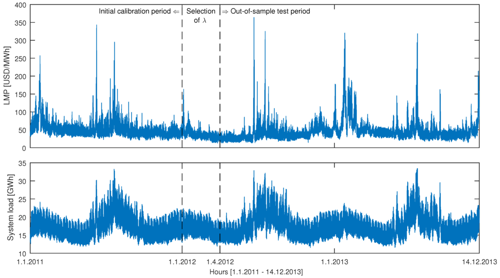
Figure 1.
GEFCom2014 hourly locational marginal prices (LMP; top) and hourly day-ahead predictions of the system load (bottom) for the period 1 January 2011–14 December 2013. The day-ahead predictions of the zonal load are generally indistinguishable from those of the system load at this resolution; see Figure 8 in [28]. The vertical dashed lines mark the beginning of the 91-day period for selecting λ’s (ridge regression, lasso, elastic nets) and the beginning of the 623-day long out-of-sample test period.
The second dataset comes from one of the major European power markets: Nord Pool (NP). It comprises hourly system prices, hourly consumption prognosis for four Nordic countries (Denmark, Finland, Norway and Sweden) and hourly wind prognosis for Denmark and covers the period 1 January 2013–29 March 2016; see Figure 2. The time series were constructed using data published by the Nordic power exchange Nord Pool (www.nordpoolspot.com) and preprocessed to account for missing values and changes to/from the daylight saving time, analogously as in [20] (Section 4.3.7). The missing data values (corresponding to the changes to the daylight saving/summer time; moreover, eight out of 28,392 hourly consumption figures were missing for Norway) were substituted by the arithmetic average of the neighboring values. The ‘doubled’ values (corresponding to the changes from the daylight saving/summer time) were substituted by the arithmetic average of the two values for the ‘doubled’ hour.
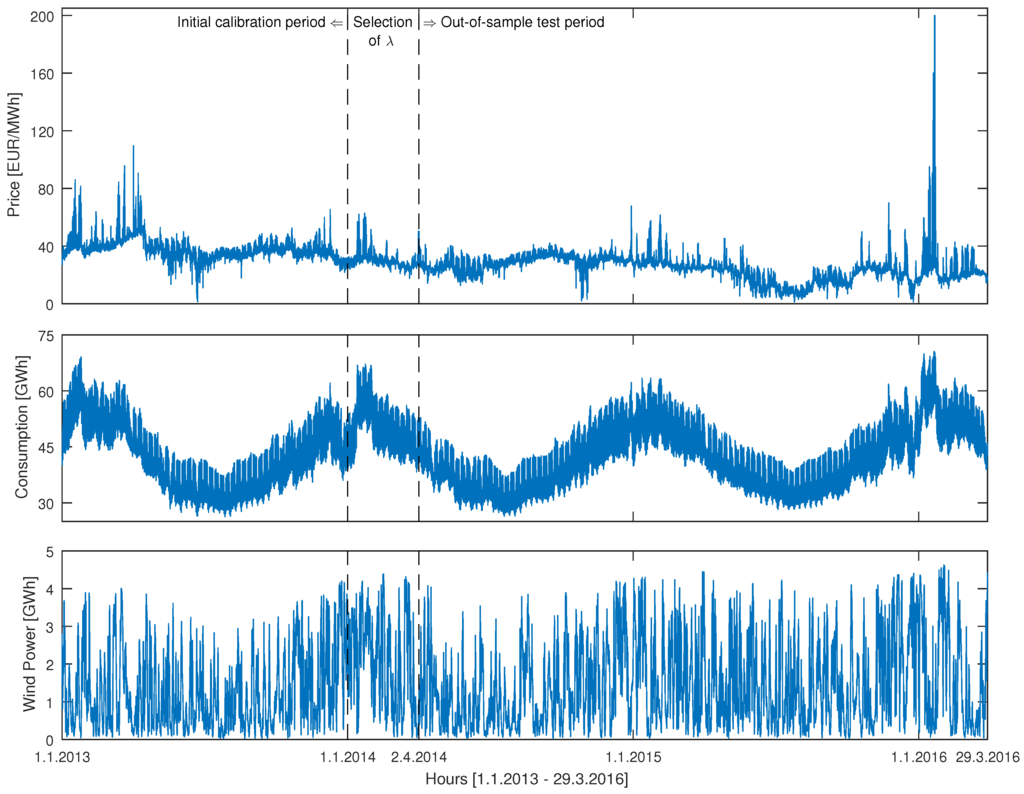
Figure 2.
Nord Pool hourly system prices (top), hourly consumption prognosis (middle) and hourly wind power prognosis for Denmark (bottom) for the period 1 January 2013–29 March 2016. The vertical dashed lines mark the beginning of the 91-day period for selecting λ’s (ridge regression, lasso, elastic net) and the beginning of the 728-day long out-of-sample test period.
The third dataset comes from N2EX, the U.K. day-ahead power market operated by Nord Pool. It comprises hourly system prices for the period 1 January 2013–29 March 2016; see Figure 3. The time series was constructed using data published by Nord Pool (www.nordpoolspot.com) and, like the second dataset, preprocessed to account for changes to/from the daylight saving time. Note that the U.K. dataset includes only prices, as no day-ahead forecasts of fundamental variables were available to us. Hence, models calibrated to the U.K. data are ‘pure price’ models. To better see the effect of excluding fundamentals from forecasting models, we use the GEFCom2014 dataset twice, once with fundamentals (system and zonal load forecasts; to compare with the results for Nord Pool) and once without them.
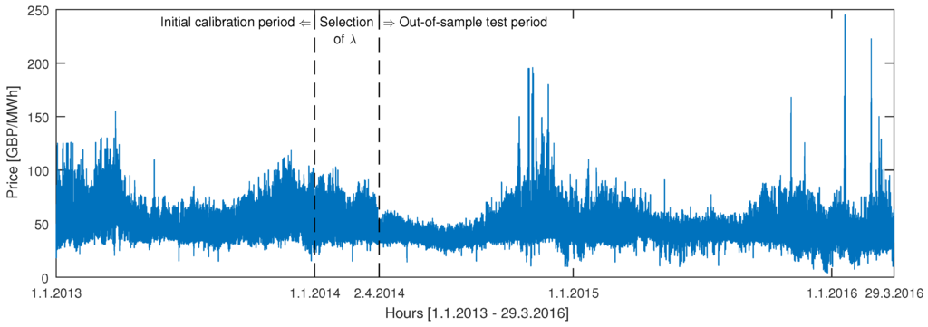
Figure 3.
U.K. power market hourly system prices (Nord Pool’s N2EX market) for the period 1 January 2013–29 March 2016. The vertical dashed lines mark the beginning of the 91-day period for selecting λ’s (ridge regression, lasso, elastic net) and the beginning of the 728-day long out-of-sample test period.
3. Methodology
It should be noted that although we use here the terms short-term, spot and day-ahead interchangeably, the former two do not necessarily refer to the day-ahead market. Short-term EPF generally involves predicting 24 hourly (or 48 half-hourly) prices in the day-ahead market, cleared typically at noon on the day before delivery, i.e., 12–36 h before delivery, the adjustment markets, cleared a few hours before delivery, and the balancing or real-time markets, cleared minutes before delivery [32]. The spot market, especially in the literature on European electricity markets, is often used as a synonym of the day-ahead market. However, in the U.S., the spot market is another name for the real-time market, while the day-ahead market is called the forward market [20,33]. Furthermore, some markets in Europe nowadays admit continuous trading for individual load periods up to a few hours before delivery. With the shifting of volume from the day-ahead to intra-day markets, also in Europe, the term spot is more and more often being used to refer to the real-time markets [1].
Throughout this article, we denote by the electricity price in the day-ahead market for day d and hour h. Like many studies in the EPF literature [1], we use the logarithmic transform to make the price series more symmetric (see Figure 4) and compare with the top panels in Figure 1, Figure 2 and Figure 3. We can do this since all considered datasets are positive-valued. However, this is not a very restrictive property. If datasets with zero or negative values were considered, we could work with non-transformed prices. Furthermore, we center the log-prices by subtracting their in-sample mean prior to parameter estimation. We do this independently for each hour :
where T is the number of days in the calibration window; hence, the missing intercept () in our autoregressive models; for model parameterizations, see Section 3.2, Section 3.3 and Section 3.4.
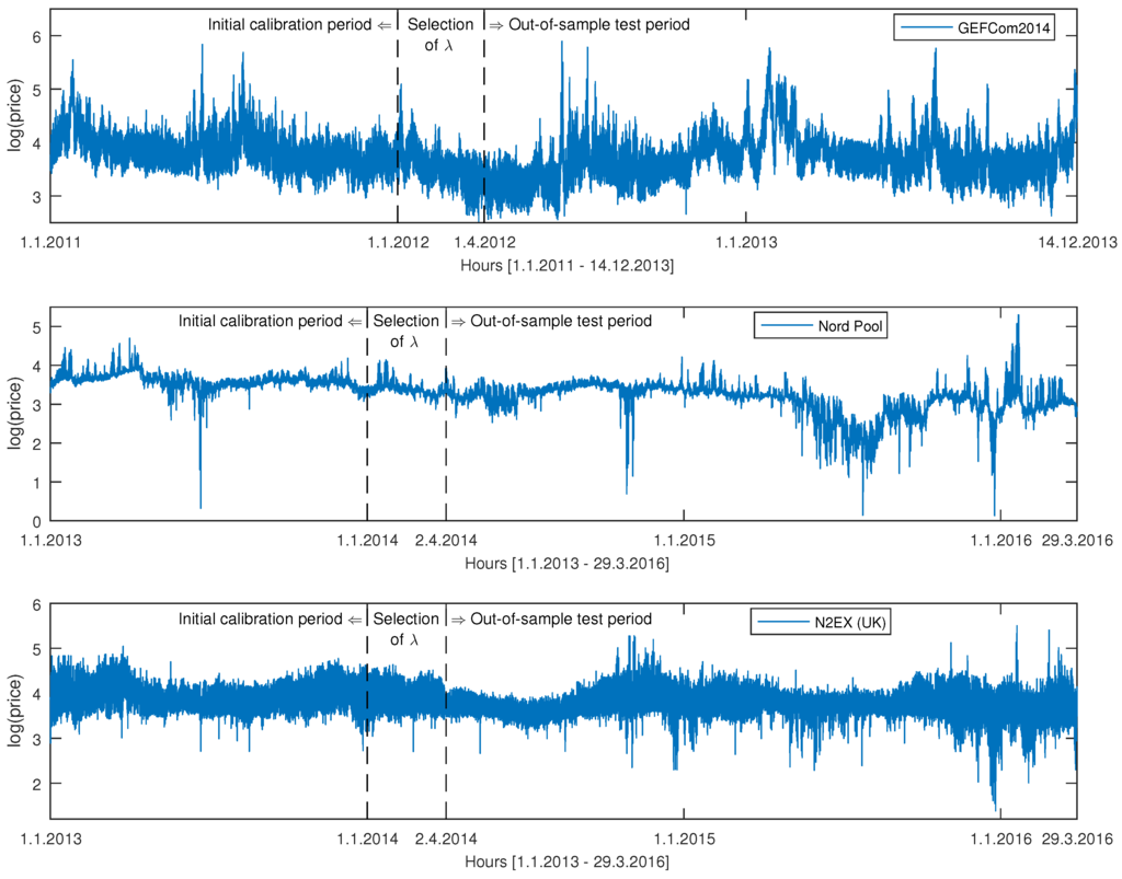
Figure 4.
Global Energy Forecasting Competition 2014 (GEFCom2014) (top), Nord Pool (middle) and N2EX (U.K.; bottom) hourly log prices. As expected, the logarithmic transform makes the price series more symmetric. The vertical dashed lines mark the beginning of the 91-day period for selecting λ’s (ridge regression, lasso, elastic nets) and the beginning of the out-of-sample test periods. Each day, the 365-day-long calibration window is rolled forward by 24 h; the models are re-estimated; and price forecasts for the 24 h of the next day are computed.
For all three markets, the day-ahead forecasts of the hourly electricity price are determined within a rolling window scheme, using a 365-day calibration window. First, all considered models are calibrated to data from the initial calibration period (i.e., 1 January 2011–31 December 2011 for GEFCom2014 and 1 January 2013–31 December 2013 for Nord Pool and the U.K.), and forecasts for all 24 h of the next day (1 January) are determined. Then, the window is rolled forward by one day; the models are re-estimated, and forecasts for all 24 h of 2 January are computed. This procedure is repeated until the predictions for the 24 h of the last day in the sample (14 December 2013 for GEFCom2014 and 29 March 2016 for Nord Pool and the U.K.) are made.
For models requiring calibration of the regularization parameter (i.e., λ), we use a setup commonly considered in the machine learning literature. Namely, we divide our datasets into estimation (365 days), validation (91 days or 13 full weeks) and test periods (623 days for GEFCom2014, 728 days for Nord Pool and the U.K.; respectively 89 and 104 full weeks). For each of the five models—ridge regression, lasso and elastic nets with , and —34 different ‘sub-models’ with 34 values of λ spanning the regularization parameter space (see Section 3.4.3 and Section 3.4.4 for details) are estimated in the 91-day validation period directly following the last day of the initial calibration period; see Figure 1, Figure 2 and Figure 3. For all hours of the day, only one value of λ is chosen for each of the five models: the one that yields the smallest error during this 91-day period; for error definitions, see Section 4.1. This value of λ is later used for computing day-ahead price forecasts in the whole out-of-sample test period. To ensure that all models are evaluated using the same data, predictions of all models are compared only in the out-of-sample test periods: 1 April 2012–14 December 2013 (623 days) for GEFCom2014 and 2 April 2014–29 March 2016 (728 days) for Nord Pool and the U.K. Obviously, such a simple procedure for the selection of the regularization parameter may not be optimal. Generally, better performance is to be expected from shrinkage models when λ is recalibrated at every time step. Such an approach has been recently taken by Ziel [18], who used the Bayesian information criterion to select one out of 50 values of λ for every day and every hour in the 969-day-long out-of-sample test period. The downside of such an approach is, however, the increased computational time.
Our choice of the model classes is guided by the existing literature on short-term EPF. Like in [12,18,25,26,27,30], the modeling is implemented separately across the hours, leading to 24 sets of parameters for each day the forecasting exercise is performed. As Ziel [18] notes, when we compare the forecasting performance of relatively simple models implemented separately across the hours and jointly for all hours (like in [9,34,35,36]), the latter generally performs better for the first half of the day, whereas the former are better in the second half of the day. At the same time, models implemented separately across the hours offer more flexibility by allowing for time-varying cross-hour dependency in a straightforward manner. Hence, our choice of the modeling framework.
In the remainder of this section, we first define the benchmarks: a simple similar-day technique and a collection of parsimonious autoregressive models. Since the latter are usually built on some prior knowledge of experts, like in [18], we refer to them as expert models. Then, we move on to describe the selection and shrinkage procedures used in this study.
3.1. The Naive Benchmark
The first benchmark, most likely introduced to the EPF literature in [34] and dubbed the naive method, belongs to the class of similar-day techniques (for a taxonomy of EPF approaches, see, e.g., [1]). It proceeds as follows: the electricity price forecast for hour h on Monday is set equal to the price for the same hour on Monday of the previous week, and the same rule applies for Saturdays and Sundays; the electricity price forecast for hour h on Tuesday is set equal to the price for the same hour on Monday, and the same rule applies for Wednesdays, Thursdays and Fridays. As was argued in [34,35], forecasting procedures that are not calibrated carefully fail to outperform the naive method surprisingly often. We denote this benchmark by Naive.
3.2. Autoregressive Expert Benchmarks
The second benchmark is a parsimonious autoregressive structure originally proposed by Misiorek et al. [19] and later used in a number of EPF studies [18,20,21,23,24,25,26,27]. Within this model, the centered log-price on day d and hour h, i.e., , is given by the following formula:
where the lagged log-prices , and account for the autoregressive effects of the previous days (the same hour yesterday, two days ago and one week ago), while is the minimum of the previous day’s 24 hourly log-prices. The exogenous variable refers to the logarithm of hourly system load or Nordic consumption for day d and hour h (actually, to forecasts made a day before, see Section 2). The three dummy variables—, and —account for the weekly seasonality. Finally, the ’s are assumed to be independent and identically distributed (i.i.d.) normal variables. We denote this autoregressive benchmark by ARX1 to reflect the fact that the load (or consumption) forecast is used as the exogenous variable in Equation (2). The corresponding model with , i.e., with no exogenous variable, is denoted by AR1. The ARX1 and AR1 models, as well as all autoregressive structures considered in Section 3.2 and Section 3.3, are estimated in this study with least squares (LS), using MATLAB’s regress.m function.
In what follows, we also consider two variants of Equation (2) that treat holidays as special days:
and that additionally utilize the fact that prices for early morning hours depend more on the previous day’s price at midnight, i.e., , than on the price for the same hour, as recently noted in [18,29]:
We denote Models (3) and (4) by ARX1h and ARX1hm, respectively. Similarly, corresponding models with are denoted by AR1h and AR1hm. Note, that when forecasting the electricity price for the last load period of the day, i.e., , models with suffix hm reduce to models with suffix h (this is true for all models considered in Section 3.2).
In Equations (3) and (4), is a dummy variable for holidays. The holidays were identified using the Time and Date AS (www.timeanddate.com/holidays) web page: U.S. federal holidays (for GEFCom2014), national holidays in Norway (for Nord Pool) and public holidays, bank holidays and major observances in the U.K. (option ‘Holidays and some observances’).
The third benchmark is an extension of the ARX1 model, which takes into account the experience gained during the GEFCom2014 competition that it may be beneficial to use different model structures for different days of the week, not only different parameter sets [29]. Hence, the multi-day ARX model (denoted later in the text by mARX1) is given by the following formula:
where , and the term accounts for the autoregressive effect of Friday’s prices on the prices for the same hour on Monday. Note that to some extent, this structure resembles periodic autoregressive moving average (PARMA) models, which have seen limited use in EPF [37,38]. Like for the ARX1 model, also for mARX1, we consider two variants:
The corresponding price only models, i.e., with , are denoted by mAR1, mAR1h and mAR1hm.
Misiorek et al. [19] noted that the minimum of the previous day’s 24 hourly prices was the best link between today’s prices and those from the entire previous day. Their analysis, however, was limited to one small dataset (California CalPXprices, 3–9 April 2000) and only one simple function at a time (maximum, minimum, mean or median of the previous day’s prices). To check if using more than one function leads to a better forecasting performance, we introduce a benchmark, which is an extension of the ARX1 model that takes into account not only the minimum , but also the maximum and the mean of the previous day’s 24 hourly prices. Additionally, we include a second exogenous variable , which is taken as either the logarithm of the day-ahead zonal load forecast (GEFCom2014) or of the Danish wind power prognosis. The resulting ARX2 model is given by the following formula:
Like for the ARX1 and mARX1 models, also for ARX2, we consider two variants:
The corresponding price only models, i.e., with , are denoted by AR2, AR2h and AR2hm.
3.3. Full Autoregressive Model
Finally, we define a much richer autoregressive model that includes as special cases all expert models discussed in Section 3.2 and call it the full ARX or fARX model. We consider all regressors that, in our opinion, posses a non-negligible predictive power. The fARX model is similar in spirit to the general autoregressive model defined by Equation (2) in [18]. However, there are some important differences between them. On one hand, fARX includes exogenous variables and a much richer seasonal structure. On the other, it does not look that far into the past and concentrates only on days , , and . The fARX model is given by the following formula:
where are dummies for the seven days of the week (we treat holidays as the eighth day of the week, hence for holidays). The price only variant, fAR, is obtained by setting to zero all coefficients of the terms involving exogenous variables, i.e., , for .
Although we fit the fARX model to power market data and evaluate its forecasting performance, the main reason for including it in this study is to use it as the baseline model for the selection and shrinkage procedures discussed in Section 3.4. For this purpose, let us write the fARX model in a more compact form:
where ’s are the regressors in Equation (7) and ’s are their coefficients.
3.4. Selection and Shrinkage Procedures
All autoregressive models considered in Section 3.2 and Section 3.3 are estimated in this study with least squares (LS). However, there are many alternatives to using LS in multi-parameter models, in particular [39]:
- variable or subset selection, which involves identifying a subset of predictors that we believe to be influential, then fitting a model using LS on the reduced set of variables,
- shrinkage (also known as regularization), which fits the full model with all predictors using an algorithm that shrinks the estimated coefficients towards zero, which can significantly reduce their variance.
Depending on what type of shrinkage is performed, some of the coefficients may be shrunk to zero itself. As such, some shrinkage methods, like the lasso, de facto perform variable selection. It should be noted, however, that variable selection (or model sparsity) is beneficial for interpretability and faster simulation of model trajectories; for reducing the forecasting errors, only the shrinkage property is required.
3.4.1. Single-Step Elimination of Insignificant Predictors
This subset selection procedure is a simple alternative to stepwise regression discussed in Section 3.4.2 and has been used, for instance, in [5]. The idea is to fit the full regression model, in our case fARX, then in a single step, set to zero all statistically insignificant coefficients. We use MATLAB’s regress.m function with the commonly-used 5% significance level. Setting to zero all coefficients in Equation (7) whose 95% confidence intervals (CI) include zero yields the ssARX model for a particular day and hour (the ssAR model is obtained analogously from fAR; see Section 3.3). This procedure can be conducted by imposing some additional constraints, for instance, leaving in the model all coefficients of the basic ARX1 (or AR1) benchmark. This yields the ssARX1 and ssAR1 models. Of course, the most commonly-used significance level of 5% may not be optimal. We have additionally checked the performance of 90% and 97.5% CI. It turns out that the overall ranking of the ssAR-type models does not change much. However, ssARX and ssAR perform slightly better for the 90% CI, while ssARX1 and ssAR1 either for the 95% or the 97.5% CI.
3.4.2. Stepwise Regression
Although very fast, the single-step elimination may remove too many explanatory variables at once and lead to a poorly-performing subset of predictors. On the other hand, selecting the best subset from among all subsets of the n predictors is not computationally feasible for large n. Even if doable, it may lead to overfitting. For these reasons, stepwise methods, which explore a far more restricted set of models, are attractive alternatives to best subset selection [39]. In the context of EPF, they have been used, for instance, in [12,13,40].
There are two basic procedures: forward selection and backward elimination. Forward stepwise selection begins with a model containing no predictors and then iteratively adds variables to the model. At each step, the variable that gives the greatest additional improvement to the fit is added to the model, and the procedure continues until all important predictors are in the model. We use MATLAB’s stepwisefit.m function, which computes the p-value of an F-statistic at each time step to test models with and without a potential term. If a variable is not currently in the model, the null hypothesis is that it would have a zero coefficient if added to the model. If there is sufficient evidence to reject the null hypothesis, that variable may be added to the model (we use stepwisefit’s default 5% significance level for adding variables; naturally, this could be further fine tuned as for the single-step elimination procedures). In a given step, the function adds the variable with the smallest p-value. We denote the resulting models by fsARX and fsAR.
Backward stepwise elimination (or selection) begins with the full model containing all n variables, i.e., fARX or fAR, and then iteratively removes the least useful predictor, one at a time. MATLAB’s stepwisefit.m function computes the null hypothesis that a given variable has a zero coefficient. If there is insufficient evidence to reject the null hypothesis, the variable may be removed from the model (we use stepwisefit’s default 10% significance level for removing variables). In a given step, the function removes the variable with the largest p-value. We denote the resulting models by bsARX and bsAR.
3.4.3. Ridge Regression
Ridge regression is a regularization method introduced in statistics by Hoerl and Kennard [41]. To our best knowledge, apart from a limited study of Barnes and Balda [16] in the context of evaluating the profitability of battery storage, the method has not been used for EPF. Ridge regression is very similar to least squares, except that the ’s in (8) are not estimated by minimizing the residual sum of squares (RSS), but by RSS penalized by a quadratic shrinkage factor:
where T represents the calibration period and is a tuning or regularization parameter, to be determined separately. Note that for , we get the standard LS estimator; for , all ’s tend to zero; while for intermediate values of λ, we are balancing two ideas: minimizing the RSS and shrinking the coefficients towards zero (and each other).
Ridge regression produces a different set of coefficient estimates for each value of λ; hence, selecting a good value for λ is critical. Cross-validation provides a simple way to tackle this problem [39]. We choose a grid of λ values (here: 34 equally-spaced values spanning the range from 1–100; if was selected, we additionally checked another set of 34 equally-spaced values spanning the range from 101–200) and using MATLAB’s ridge.m function (we scale the regressors) compute the prediction errors for each value of the tuning parameter in the 91-day validation period; see Section 2. We then select λ for which the error (for the definition, see Section 4.1) is the smallest and use it for computing day-ahead price forecasts in the whole out-of-sample test period. The resulting model is denoted in the text by RidgeX or Ridge when the baseline model is fAR.
3.4.4. Lasso and Elastic Nets
Ridge regression has one unwanted feature when it comes to interpretation and model identification. Unlike stepwise regression, which will generally select models that involve just a subset of the variables, ridge regression will include all n predictors in the final model [39]. The quadratic shrinkage factor in Equation (9) will shrink all ’s towards zero, but it will not set any of them exactly to zero. In 1996, Tibshirani [42] proposed the least absolute shrinkage and selection operator (i.e., lasso or LASSO) that overcomes this disadvantage. It is the only shrinkage procedure that has been applied in EPF to a larger extent, however only in the last two years [7,9,18,25,43].
The lasso is a shrinkage method just like ridge regression. However, it uses a linear penalty factor instead of a quadratic one:
This subtle change makes the solutions nonlinear in , and there is no closed form expression as in the case of ridge regression. Because of the nature of the shrinkage factor in Equation (10), making λ sufficiently large will cause some of the coefficients to be exactly zero [44]. Thus, the lasso de facto performs variable selection, just like the methods discussed in Section 3.4.1 and Section 3.4.2. As in ridge regression, selecting a good value of λ for the lasso is critical. Here, we use MATLAB’s lasso.m function and a grid of exponentially-decreasing λ’s (the largest just sufficient to produce all ; the function also automatically scales the regressors). We then select λ for which the error (for the definition, see Section 4.1) in the 91-day validation period is the smallest. The resulting model is denoted in the text by LassoX, or Lasso when the baseline model is fAR.
The lasso does not handle highly-correlated variables very well. The coefficient paths tend to be erratic and can sometimes show wild behavior [44]. This is not a critical issue for forecasting, but for interpretation and model identification, this has more serious consequences. In 2005, Zou and Hastie [45] proposed the elastic net, a new regularization and variable selection method that can be seen as an extension of ridge regression and the lasso. It often outperforms the lasso, while exhibiting a similar sparsity of representation. The elastic net uses a mixture of linear and quadratic penalty factors:
where . When , the elastic net reduces to the lasso, and with , it becomes ridge regression. The in the quadratic part of the elastic net penalty in Equation (11) leads to a more efficient and intuitive soft-thresholding operator in the optimization; the original formulation in [45] did not include the scaling. Note also that every elastic net problem can be rewritten as a lasso problem on augmented data. Hence, for fixed λ and α, the computational difficulty of the elastic net solution is similar to the lasso problem [44].
Compared to the lasso and ridge regression, the elastic net has an additional mixing parameter that has to be determined. It can be set on subjective grounds, as we do here, or optimized within a cross-validation scheme. We use MATLAB’s lasso.m function (with a grid of exponentially-decreasing λ’s; the function also automatically scales the regressors) and three values of the mixing parameter, , and . This yields six elastic net models:
- EN25X, EN50X and EN75X when the baseline model is fARX,
- and EN25, EN50 and EN75 when the baseline model is fAR,
4. Empirical Results
We now present day-ahead forecasting results for the three considered datasets: GEFCom2014 hourly locational marginal prices, Nord Pool hourly system prices and U.K. hourly system prices. We use long, two-year out-of-sample test periods to make sure the obtained results are reliable (for the GEFCom2014 dataset, the test period is shorter: 623 days; see Figure 1). Recall from Section 2 that the models are re-estimated on a daily basis. Price forecasts for all 24 h of the next day are determined at the same point in time, and the 365-day calibration window is rolled forward by one day.
4.1. Performance Evaluation in Terms of WMAE
Following [21,24,30,35], we compare the models in terms of the weekly-weighted mean absolute error (WMAE) loss function, which is a robust measure similar to MAPE, but with the absolute error normalized by the mean weekly price to avoid the adverse effect of negative and close to zero electricity spot prices. We evaluate the forecasting performance using weekly time intervals, each with hourly observations. For each week in the out-of-sample test period, we calculate the error for each model as:
where is the actual price for hour h (not the centered log-price ), is the model predicted price for that hour, is the mean price for a given week and for GEFCom2014 and 104 for Nord Pool and the U.K. Next, we aggregate these errors into one mean value over all weeks in the out-of-sample test period:
Note that we also analyzed the forecasts using the weekly root mean square error (see [1] (Section 3.3)), but the results were qualitatively the same and are omitted here due to space limitations.
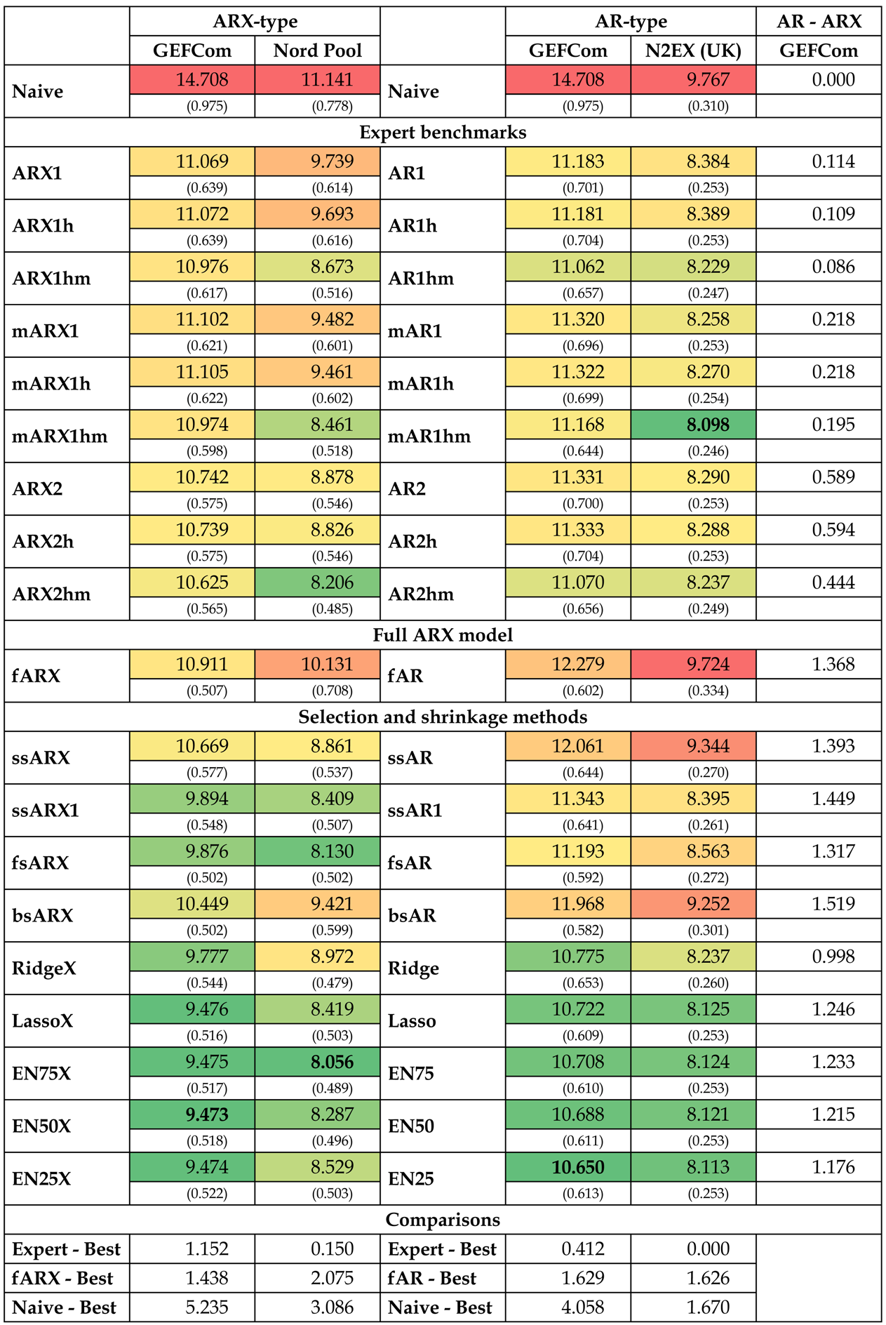
In Table 1, we report errors for the three considered datasets and the 20 model types. We use the GEFCom2014 dataset twice: once we fit ARX-type models to the complete dataset with exogenous variables (system and zonal load; left part of the table) and once we fit AR-type models to the dataset without them (right part of the table). This allows us to compute the decrease in WMAE when exogenous variables are added to the model (the last column in Table 1). Several important conclusions can be drawn:
- All models beat the Naive benchmark and, except for the fAR model and the U.K. data, by a large margin. In particular, the improvement from using elastic nets can be as much as 5%! This indicates that they all are highly efficient forecasting tools.
- When we exclude single-step elimination without constraints (ssAR/X) and backward selection (bsAR/X) models, the selection and shrinkage methods generally outperform the expert benchmarks. In particular, the elastic net model with (i.e., closer in terms of α to the lasso than to ridge regression) beats every expert model, except mAR1hm for the U.K. data, where it is second best.
- The latter comment leads us to the next conclusion that adding the price for the last load period of the day, , to the expert models improves their performance greatly. This fact has been recognized in the EPF literature only very recently [18,25,29] and apparently requires more attention. To see this, compare the models with suffix m to those without it. In particular, mAR1hm is the overall best performing model for the U.K. dataset and ARX2hm is the third best model for the Nord Pool dataset.
- Somewhat surprisingly, the full ARX model performs poorly. For the U.K. dataset, it is nearly as bad as the Naive benchmark. In all four cases (three datasets + GEFCom2014 without exogenous variables), it is worse than the overall best model and the best performing elastic net (EN75/X) by at least 1.4%. Given that a 1% improvement in MAPE translates into savings of ca. $1.5 million per year for a typical medium-size utility [2,3], this observation is of high practical value. Yet, from a statistical perspective, this finding is not that surprising. The fARX model has 107 parameters, which have to be calibrated to only 365 observations. Increasing the length of the calibration window should lead to a better performance of the full model.
- Among the selection and shrinkage methods, the lasso and elastic nets tend to outperform single-step elimination (ssAR/X/1), stepwise regression (fsAR/X, bsAR/X) and even ridge regression (Ridge/X). Only for the Nord Pool dataset, the fsARX forward selection model is better than the lasso and two elastic nets.

Table 1.
Mean values of the weekly-weighted mean absolute errors, i.e., defined by Equation (13), over all 89 weeks of the GEFCom2014 or all 104 weeks of the Nord Pool and U.K. out-of-sample test periods. errors are reported in percent, with standard deviation in parentheses. A heat map is used to indicate better (→ green) and worse (→ red) performing models. errors for the best performing model for each dataset are emphasized in bold. The last column presents the decrease in when exogenous variables are added to the model (AR→ ARX; for the GEFCom2014 dataset). The bottom rows compare the performance across model classes.
4.2. Diebold–Mariano Tests
In order to formally investigate the advantages from using selection and shrinkage methods, we apply the Diebold–Mariano (DM; see [31]) test for significant differences in the forecasting performance. Since predictions for all 24 h of the next day are made at the same time using the same information set, forecast errors for a particular day will typically exhibit high serial correlation. Therefore, like [24,30,46], we conduct the DM tests for each of the 24 load periods separately, using absolute error losses of the model forecast:
For each pair of models and for each hour independently, we calculate the loss differential series:
We perform two one-sided DM tests at the 5% significance level: (i) a test with the null hypothesis , i.e., the outperformance of the forecasts of by those of ; and (ii) the complementary test with the reverse null , i.e., the outperformance of the forecasts of by those of . Note that, like in [24,30,46], we assume here forecasts for consecutive days, hence loss differentials are not serially correlated. For the better performing models, this is a generally valid assumption.
In Figure 5 and Figure 6, we summarize the DM results for all test cases (three datasets + GEFCom2014 without exogenous variables). Namely, we sum the number of significant differences in forecasting performance across the 24 h and use a heat map to indicate the number of hours for which the forecasts of a model on the X-axis are significantly better than those of a model on the Y-axis. Two extreme cases—(i) the forecasts of a model on the X-axis are significantly better for all 24 h of the day and (ii) the forecasts of a model on the X-axis are not significantly better for any hour—are indicated by white and black squares, respectively. Naturally, the diagonal (white crosses on black squares) should be ignored, as it concerns the same model on both axes. Columns with many non-black squares (the more green or white the better) indicate that the forecasts of a model on the X-axis are significantly better than the forecasts of many of its competitors. Conversely, rows with many non-black squares mean that the forecasts of a model on the Y-axis are significantly worse than the forecasts of many of its competitors. For instance, for the GEFCom2014 dataset and ARX-type models displayed in the left panel of Figure 5, the white row for the Naive benchmark indicates that the forecasts of this simple model are significantly worse than the forecasts of all of its competitors for all 24 h, while the black column for the Naive benchmark means that not a single competitor produces significantly worse forecasts than Naive, even for a single hour of the day.
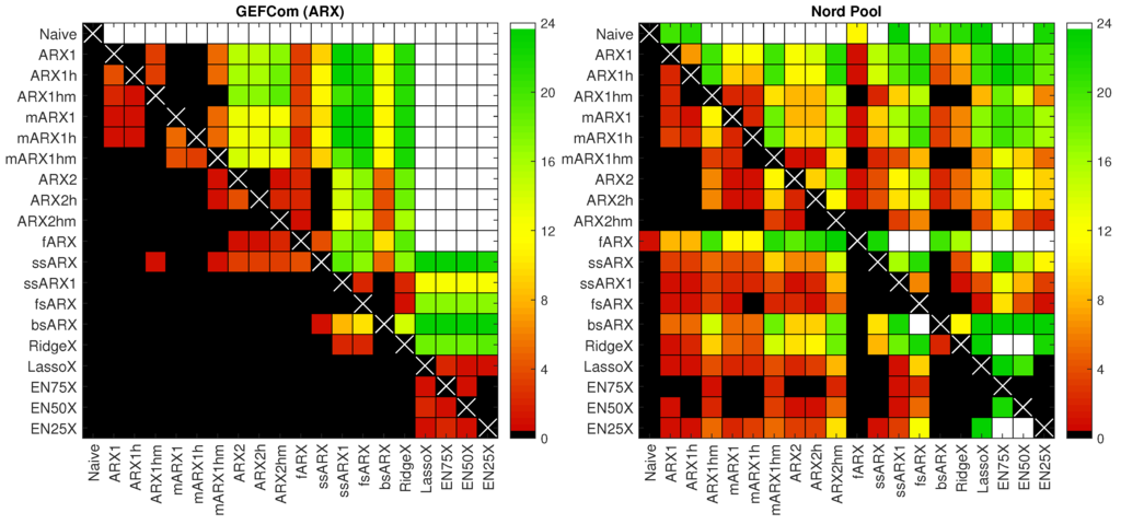
Figure 5.
Results for conducted one-sided Diebold–Mariano tests at the 5% level for autoregressive model structures with exogenous variables (ARX)-type models and two datasets: GEFCom2014 (left panel) and Nord Pool (right panel). We sum the number of significant differences in forecasting performance across the 24 h and use a heat map to indicate the number of hours for which the forecasts of a model on the X-axis are significantly better than those of a model on the Y-axis. A white square indicates that forecasts of a model on the X-axis are better for all 24 h, while a black square that they are not better for a single hour.
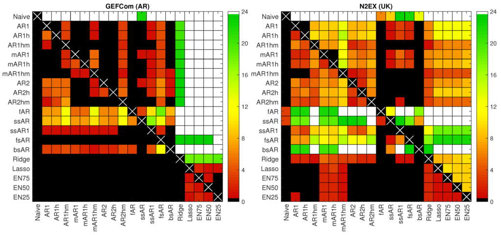
Figure 6.
Results for conducted one-sided Diebold–Mariano tests at the 5% level for AR-type models and two datasets: GEFCom2014 (left panel) and N2EX (U.K.; right panel). We sum the number of significant differences in forecasting performance across the 24 h and use a heat map to indicate the number of hours for which the forecasts of a model on the X-axis are significantly better than those of a model on the Y-axis. A white square indicates that forecasts of a model on the X-axis are better for all 24 h, while a black square that they are not better for a single hour.
The obtained DM-test results support our observations from Section 4.1 on WMAE errors. Again, we can conclude that applying the lasso or one of the elastic nets improves forecasting accuracy. Especially for the GEFCom2014 dataset (both for ARX- and AR-type models), these variable selection schemes lead to models that yield significantly better forecasts than those of the expert models (see the white columns for Lasso/X, EN75/X, EN50/X and EN25/X in the left panels of Figure 5 and Figure 6), while their predictions are never outperformed by any of the competitors (see the black rows for these four models). For the Nord Pool and U.K. datasets, the results are not that clear cut, but still there are many more green or white squares in the columns than in the rows corresponding to these four selection schemes.
Again, EN75/X stands out as the best performing model overall. For the GEFCom2014 test cases, it always leads to significantly better forecasts than any of the expert benchmarks. For the Nord Pool dataset, its forecasts are significantly better for 10–23 h of the day and significantly worse for at most 2 h (only for models with suffix m: mARX1hm and ARX2hm, 2 h, and ARX1hm, 1 h). Finally, for the U.K. dataset, the results are the least convincing. EN75/X yields significantly better forecasts for 4–12 h of the day and significantly worse for at most 2 h (only for mAR-type models: mAR1 and mAR1h, 2 h, and mAR1hm, 1 h).
Now, let us look in detail at the performance for each hour of the day. In Figure 7, we provide a graphical representation of the DM test statistic for four models and all considered datasets. The models include: the best overall EN75/X model and three benchmarks (Naive, mARX1hm/mAR1hm and fAR/X). For the GEFCom2014 dataset, EN75/X clearly beats all benchmarks across all hours. The situation for the remaining two datasets would be nearly the same if it was not for the early morning hours (Hours 6 and 7 for Nord Pool and Hour 8 for the U.K.), when the expert benchmarks yield significantly better predictions. This is somewhat surprising, since the morning peak comes a bit later in both markets. Perhaps looking at variables selected by the elastic net algorithm will provide more insight.
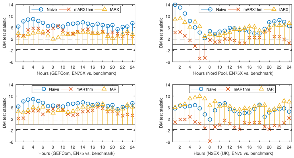
Figure 7.
Results for the conducted one-sided Diebold–Mariano tests at the 5% significance level for selected ARX-type models and the GEFCom2014 and Nord Pool datasets (top panels) and selected AR-type models and the GEFCom2014 and N2EX (U.K.) datasets (bottom panels). The tests were conducted separately for each of the 24 h. The figures report the value of the test statistic for each test, as well as two thresholds (dashed lines in the plots). The lower one refers to null hypothesis , i.e., the outperformance of the forecasts of EN75/X by those of a given benchmark (Naive, mARX1hm/mAR1hm, fAR/X). The upper threshold refers to the complementary test with the reverse null, i.e., or the outperformance of the forecasts of a given benchmark by those of EN75/X. Only points lying below (or above) the dashed threshold lines are significant at the 5% level. See also Figure 5 and Figure 6.
4.3. Variable Selection
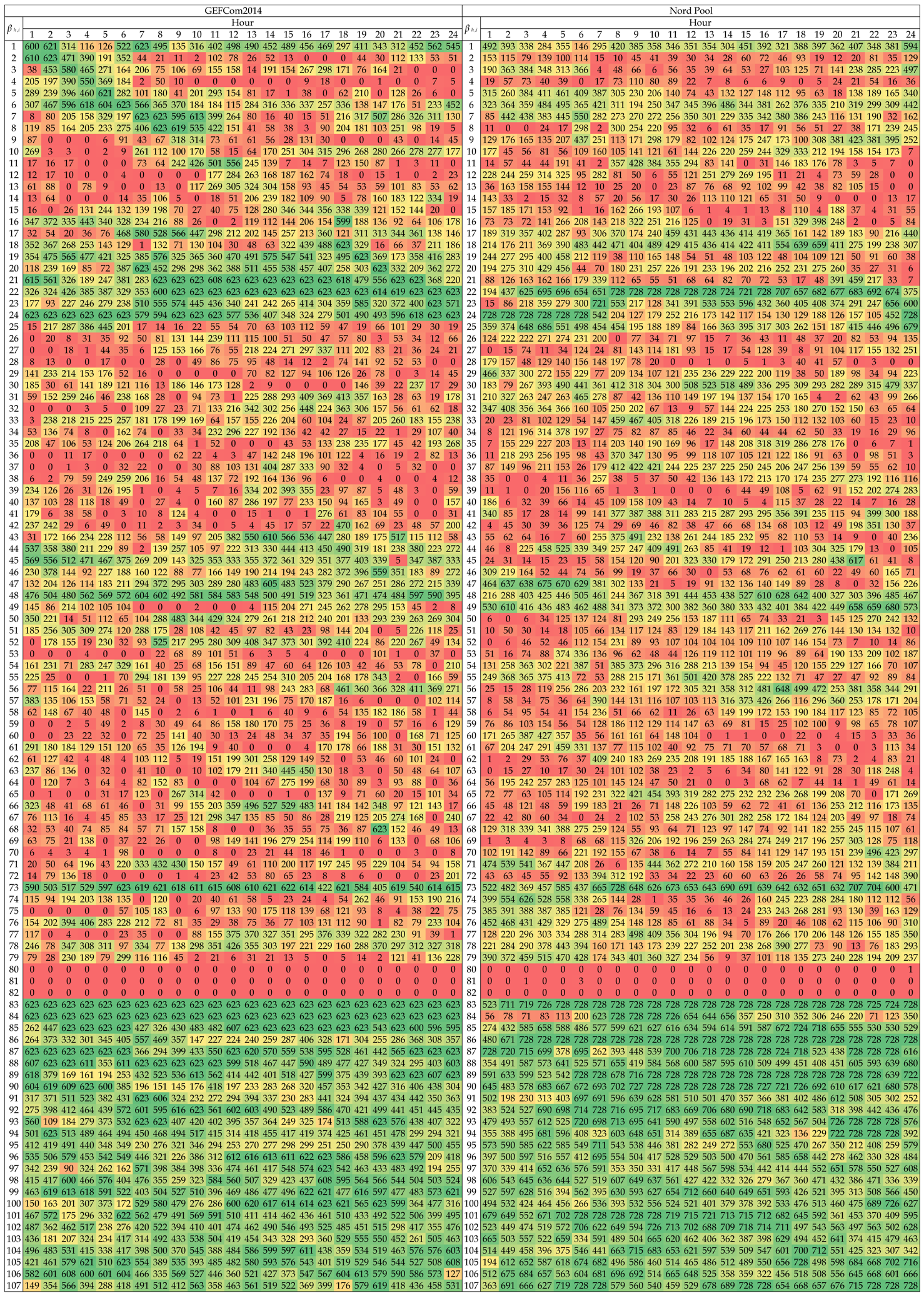
In Table 2 and Table 3, we provide the number of days in the out-of-sample test period for which a given was selected for the best performing elastic net model, i.e., EN75/X. The maximum number of days is 623 ( weeks) for GEFCom2014 and 728 ( weeks) for Nord Pool and N2EX (U.K.). A heat map is used to indicate more (→ green) and less (→ red) commonly-selected ’s. The ’s are numbered as in Equation (7). Note that in the EN75 model; see Table 3. Several interesting conclusions can be drawn:
- There is no single variable that is always used, regardless of the dataset, hour of the day or the day in the out-of-sample test period. The closest to ‘perfection’ is the day-ahead load forecast for the predicted hour, i.e., (see Row 83 in Table 2). Surprisingly, this dependence on the load forecast is stronger than the autoregressive effect (see the next bullet point). This may be a hint that the load-price relationship should be given more attention and that functionals of load-related (or other fundamental) variables should be included in EPF models, like in [10].
- As expected, the price 24 h ago, i.e., , is an influential variable; see the diagonals in Rows 1–24 in both Tables. However, it is not only the same hour a day earlier, but also the neighboring hours. The diagonal is less visible around mid-day, and for Nord Pool, it almost disappears except for the late night hours. The latter may be to some extent due to the importance of wind in this market and the explanatory power of the day-ahead wind prognosis for the predicted hour.
- As recently observed in [18,29], the price for Hour 24, i.e., , is an influential variable. Somewhat surprisingly, sometime between 7–9 a.m. and 9–11 p.m., Hour 22, i.e., , becomes more important. What is more surprising, these late night hours are generally more often selected than the same hour a day ago, i.e., . These observations require more thorough studies. Nevertheless, our limited results suggest that these late hour variables should be taken into account when constructing expert models.
- Clearly, the least important variables for all markets are the daily average prices over the last three days, i.e., for , which are almost never selected. There are some exceptions, though, for the GEFCom2014 dataset and the EN75 model; see Table 3. Of the two other aggregated variables, is slightly more influential than , which contradicts the observations of Misiorek et al. [19] and may suggest its use in expert models instead of the minimum.
- If prices from days or are ever selected, it is only for hours around midnight the day before (i.e., , , ) or similar hours (i.e., the diagonals in Rows 25–48 and 49–72). On the other hand, the same hour one week ago, i.e., , has a high explanatory power (see Row 73 for all datasets), which justifies its use in expert models [18,19,20,21,22,23,30].
- Finally, the weekly dummies (Rows 87–93), the dummy-linked load forecasts (Rows 94–100 in Table 2 only) and the dummy-linked last day’s prices (Rows 101–107) are generally selected for the EN75/X model. This may be an indication that the weekly seasonality requires better modeling than offered by typically-used expert models.
Table 2.
The number of days in the out-of-sample test period for which a given (see Equation (7)) was selected for the EN75X model. The maximum number of days is 623 ( weeks) for GEFCom2014 and 728 ( weeks) for Nord Pool. A heat map is used to indicate more (→ green) and less (→ red) commonly-selected ’s.
Table 3.
The number of days in the out-of-sample test period for which a given (see Equation (7)) was selected for the EN75 model. The maximum number of days is 623 ( weeks) for GEFCom2014 and 728 ( weeks) for N2EX (U.K.). A heat map is used to indicate more (→ green) and less (→ red) commonly-selected ’s. Note that in the EN75 model.
5. Conclusions
A key point in electricity price forecasting (EPF) is the appropriate choice of explanatory variables. The typical approach has been to select predictors in an ad hoc fashion, sometimes using expert knowledge, but very rarely based on formal selection or shrinkage procedures. However, is this the right approach? Can the application of automated selection and shrinkage procedures to large sets of explanatory variables lead to better forecasts than those of the commonly-used expert models?
Conducting an empirical study involving state-of-the-art parsimonious autoregressive structures as benchmarks, datasets from three major power markets and five classes of automated selection and shrinkage procedures (single-step elimination, stepwise regression, ridge regression, lasso and elastic nets), we have addressed these important questions. To this end, we have compared the predictive performance of 20 types of models over three two-year-long out-of-sample test periods in terms of the robust weekly-weighted mean absolute error (WMAE) and tested the statistical significance of the results using the Diebold–Mariano [31] test.
We have shown that two classes of selection and shrinkage procedures—the lasso and elastic nets—lead to on average better performance than any of the considered expert benchmarks. On the other hand, single-step elimination, stepwise regression and ridge regression are not recommended for EPF as they do not yield significant accuracy gains compared to well-structured parsimonious autoregressive models. The lasso has been recently shown to perform well in EPF [9,18], but it is the more flexible elastic net that stands out as the best performing model overall. Given that both are automated procedures that do not require advanced expert knowledge or supervision, our results may have far reaching consequences for the practice of electricity price forecasting.
We have also looked at variables selected by the elastic net algorithm to gain insights for constructing efficient parsimonious models. In particular, we have confirmed the high explanatory power of the load forecasts for the target hour, of last day’s prices for the same or neighboring hours and of the price for the same hour a week earlier. Somewhat surprisingly, we have found that not only the last available data point (price for Hour 24), but also prices for Hours 21–23 of the previous day should be considered when building expert models.
Acknowledgments
The study was partially supported by the National Science Center (NCN, Poland) through Grants 2015/17/B/HS4/00334 (to Bartosz Uniejewski and Rafał Weron) and 2013/11/N/HS4/03649 (to Jakub Nowotarski).
Author Contributions
All authors conceived of and designed the forecasting study. Bartosz Uniejewski performed the numerical experiments. Jakub Nowotarski and Rafał Weron supervised the experiments. All authors analyzed the results and contributed to writing the paper.
Conflicts of Interest
The authors declare no conflict of interest.
References
- Weron, R. Electricity price forecasting: A review of the state-of-the-art with a look into the future. Int. J. Forecast. 2014, 30, 1030–1081. [Google Scholar]
- Zareipour, H.; Canizares, C.A.; Bhattacharya, K. Economic impact of electricity market price forecasting errors: A demand-side analysis. IEEE Trans. Power Syst. 2010, 25, 254–262. [Google Scholar] [CrossRef]
- Hong, T. Crystal Ball Lessons in Predictive Analytics. EnergyBiz Mag. 2015, 35–37. [Google Scholar]
- Amjady, N.; Keynia, F. Day-ahead price forecasting of electricity markets by mutual information technique and cascaded neuro-evolutionary algorithm. IEEE Trans. Power Syst. 2009, 24, 306–318. [Google Scholar] [CrossRef]
- Gianfreda, A.; Grossi, L. Forecasting Italian electricity zonal prices with exogenous variables. Energy Econ. 2012, 34, 2228–2239. [Google Scholar] [CrossRef]
- Maciejowska, K. Fundamental and speculative shocks, what drives electricity prices? In Proceedings of the 11th International Conference on the European Energy Market (EEM14), Kraków, Poland, 28–30 May 2014. [CrossRef]
- Ludwig, N.; Feuerriegel, S.; Neumann, D. Putting Big Data analytics to work: Feature selection for forecasting electricity prices using the LASSO and random forests. J. Decis. Syst. 2015, 24, 19–36. [Google Scholar] [CrossRef]
- Monteiro, C.; Fernandez-Jimenez, L.A.; Ramirez-Rosado, I.J. Explanatory information analysis for day-ahead price forecasting in the Iberian electricity market. Energies 2015, 8, 10464–10486. [Google Scholar] [CrossRef]
- Ziel, F.; Steinert, R.; Husmann, S. Efficient modeling and forecasting of electricity spot prices. Energy Econ. 2015, 47, 89–111. [Google Scholar] [CrossRef]
- Dudek, G. Multilayer perceptron for GEFCom2014 probabilistic electricity price forecasting. Int. J. Forecast. 2016, 32, 1057–1060. [Google Scholar] [CrossRef]
- Keles, D.; Scelle, J.; Paraschiv, F.; Fichtner, W. Extended forecast methods for day-ahead electricity spot prices applying artificial neural networks. Appl. Energy 2016, 162, 218–230. [Google Scholar] [CrossRef]
- Karakatsani, N.; Bunn, D. Forecasting electricity prices: The impact of fundamentals and time-varying coefficients. Int. J. Forecast. 2008, 24, 764–785. [Google Scholar] [CrossRef]
- Misiorek, A. Short-term forecasting of electricity prices: Do we need a different model for each hour? Medium Econom. Toepass. 2008, 16, 8–13. [Google Scholar]
- Amjady, N.; Keynia, F. Electricity market price spike analysis by a hybrid data model and feature selection technique. Electr. Power Syst. Res. 2010, 80, 318–327. [Google Scholar] [CrossRef]
- Voronin, S.; Partanen, J. Price forecasting in the day-ahead energy market by an iterative method with separate normal price and price spike frameworks. Energies 2013, 6, 5897–5920. [Google Scholar] [CrossRef]
- Barnes, A.K.; Balda, J.C. Sizing and economic assessment of energy storage with real-time pricing and ancillary services. In Proceedings of the 2013 4th IEEE International Symposium on Power Electronics for Distributed Generation Systems (PEDG), Rogers, AR, USA, 8–11 July 2013. [CrossRef]
- González, C.; Mira-McWilliams, J.; Juárez, I. Important variable assessment and electricity price forecasting based on regression tree models: Classification and regression trees, bagging and random forests. IET Gener. Transm. Distrib. 2015, 9, 1120–1128. [Google Scholar] [CrossRef]
- Ziel, F. Forecasting Electricity Spot Prices Using LASSO: On Capturing the Autoregressive Intraday Structure. IEEE Trans. Power Syst. 2016. [Google Scholar] [CrossRef]
- Misiorek, A.; Trück, S.; Weron, R. Point and interval forecasting of spot electricity prices: Linear vs. non-linear time series models. Stud. Nonlinear Dyn. Econom. 2006, 10. [Google Scholar] [CrossRef]
- Weron, R. Modeling and Forecasting Electricity Loads and Prices: A Statistical Approach; John Wiley & Sons: Chichester, UK, 2006. [Google Scholar]
- Weron, R.; Misiorek, A. Forecasting spot electricity prices: A comparison of parametric and semiparametric time series models. Int. J. Forecast. 2008, 24, 744–763. [Google Scholar] [CrossRef]
- Serinaldi, F. Distributional modeling and short-term forecasting of electricity prices by Generalized Additive Models for Location, Scale and Shape. Energy Econ. 2011, 33, 1216–1226. [Google Scholar] [CrossRef]
- Kristiansen, T. Forecasting Nord Pool day-ahead prices with an autoregressive model. Energy Policy 2012, 49, 328–332. [Google Scholar] [CrossRef]
- Nowotarski, J.; Raviv, E.; Trück, S.; Weron, R. An empirical comparison of alternate schemes for combining electricity spot price forecasts. Energy Econ. 2014, 46, 395–412. [Google Scholar] [CrossRef]
- Gaillard, P.; Goude, Y.; Nedellec, R. Additive models and robust aggregation for GEFCom2014 probabilistic electric load and electricity price forecasting. Int. J. Forecast. 2016, 32, 1038–1050. [Google Scholar] [CrossRef]
- Maciejowska, K.; Nowotarski, J.; Weron, R. Probabilistic forecasting of electricity spot prices using factor quantile regression averaging. Int. J. Forecast. 2016, 32, 957–965. [Google Scholar] [CrossRef]
- Nowotarski, J.; Weron, R. To combine or not to combine? Recent trends in electricity price forecasting. ARGO 2016, 9, 7–14. [Google Scholar]
- Hong, T.; Pinson, P.; Fan, S.; Zareipour, H.; Troccoli, A.; Hyndman, R.J. Probabilistic energy forecasting: Global Energy Forecasting Competition 2014 and beyond. Int. J. Forecast. 2016, 32, 896–913. [Google Scholar] [CrossRef]
- Maciejowska, K.; Nowotarski, J. A hybrid model for GEFCom2014 probabilistic electricity price forecasting. Int. J. Forecast. 2016, 32, 1051–1056. [Google Scholar] [CrossRef]
- Nowotarski, J.; Weron, R. On the importance of the long-term seasonal component in day-ahead electricity price forecasting. Energy Econ. 2016, 57, 228–235. [Google Scholar] [CrossRef]
- Diebold, F.X.; Mariano, R.S. Comparing predictive accuracy. J. Bus. Econ. Stat. 1995, 13, 253–263. [Google Scholar]
- Garcia-Martos, C.; Conejo, A. Price forecasting techniques in power systems. In Wiley Encyclopedia of Electrical and Electronics Engineering; Wiley: Chichester, UK, 2013; pp. 1–23. [Google Scholar] [CrossRef]
- Burger, M.; Graeber, B.; Schindlmayr, G. Managing Energy Risk: An Integrated View on Power and Other Energy Markets; Wiley: Chichester, UK, 2007. [Google Scholar]
- Nogales, F.J.; Contreras, J.; Conejo, A.J.; Espinola, R. Forecasting next-day electricity prices by time series models. IEEE Trans. Power Syst. 2002, 17, 342–348. [Google Scholar] [CrossRef]
- Conejo, A.J.; Contreras, J.; Espínola, R.; Plazas, M.A. Forecasting electricity prices for a day-ahead pool-based electric energy market. Int. J. Forecast. 2005, 21, 435–462. [Google Scholar] [CrossRef]
- Paraschiv, F.; Fleten, S.E.; Schürle, M. A spot-forward model for electricity prices with regime shifts. Energy Econ. 2015, 47, 142–153. [Google Scholar] [CrossRef]
- Broszkiewicz-Suwaj, E.; Makagon, A.; Weron, R.; Wyłomańska, A. On detecting and modeling periodic correlation in financial data. Physica A 2004, 336, 196–205. [Google Scholar] [CrossRef]
- Bosco, B.; Parisio, L.; Pelagatti, M. Deregulated wholesale electricity prices in Italy: An empirical analysis. Int. Adv. Econ. Res. 2007, 13, 415–432. [Google Scholar] [CrossRef]
- James, G.; Witten, D.; Hastie, T.; Tibshirani, R. An Introduction to Statistical Learning with Applications in R; Springer: New York, NY, USA, 2013. [Google Scholar]
- Bessec, M.; Fouquau, J.; Meritet, S. Forecasting electricity spot prices using time-series models with a double temporal segmentation. Appl. Econ. 2016, 48, 361–378. [Google Scholar] [CrossRef]
- Hoerl, A.E.; Kennard, R.W. Ridge regression: Biased estimation for nonorthogonal problems. Technometrics 1970, 12, 55–67. [Google Scholar] [CrossRef]
- Tibshirani, R. Regression shrinkage and selection via the lasso. J. Royal Stat. Soc. B 1996, 58, 267–288. [Google Scholar]
- Ziel, F. Iteratively reweighted adaptive lasso for conditional heteroscedastic time series with applications to AR-ARCH type processes. Comput. Stat. Data Anal. 2016, 100, 773–793. [Google Scholar] [CrossRef]
- Hastie, T.; Tibshirani, R.; Wainwright, M. Statistical Learning with Sparsity: The Lasso and Generalizations; CRC Press: Philadelphia, PA, USA, 2015. [Google Scholar]
- Zou, H.; Hastie, T. Regularization and Variable Selection via the Elastic Nets. J. Royal Stat. Soc. B 2015, 67, 301–320. [Google Scholar] [CrossRef]
- Bordignon, S.; Bunn, D.W.; Lisi, F.; Nan, F. Combining day-ahead forecasts for British electricity prices. Energy Econ. 2013, 35, 88–103. [Google Scholar] [CrossRef]

© 2016 by the authors; licensee MDPI, Basel, Switzerland. This article is an open access article distributed under the terms and conditions of the Creative Commons Attribution (CC-BY) license (http://creativecommons.org/licenses/by/4.0/).