
The Influence of Environmental Constraints on the Water Value †

Abstract
:1. Introduction
2. Optimisation Model
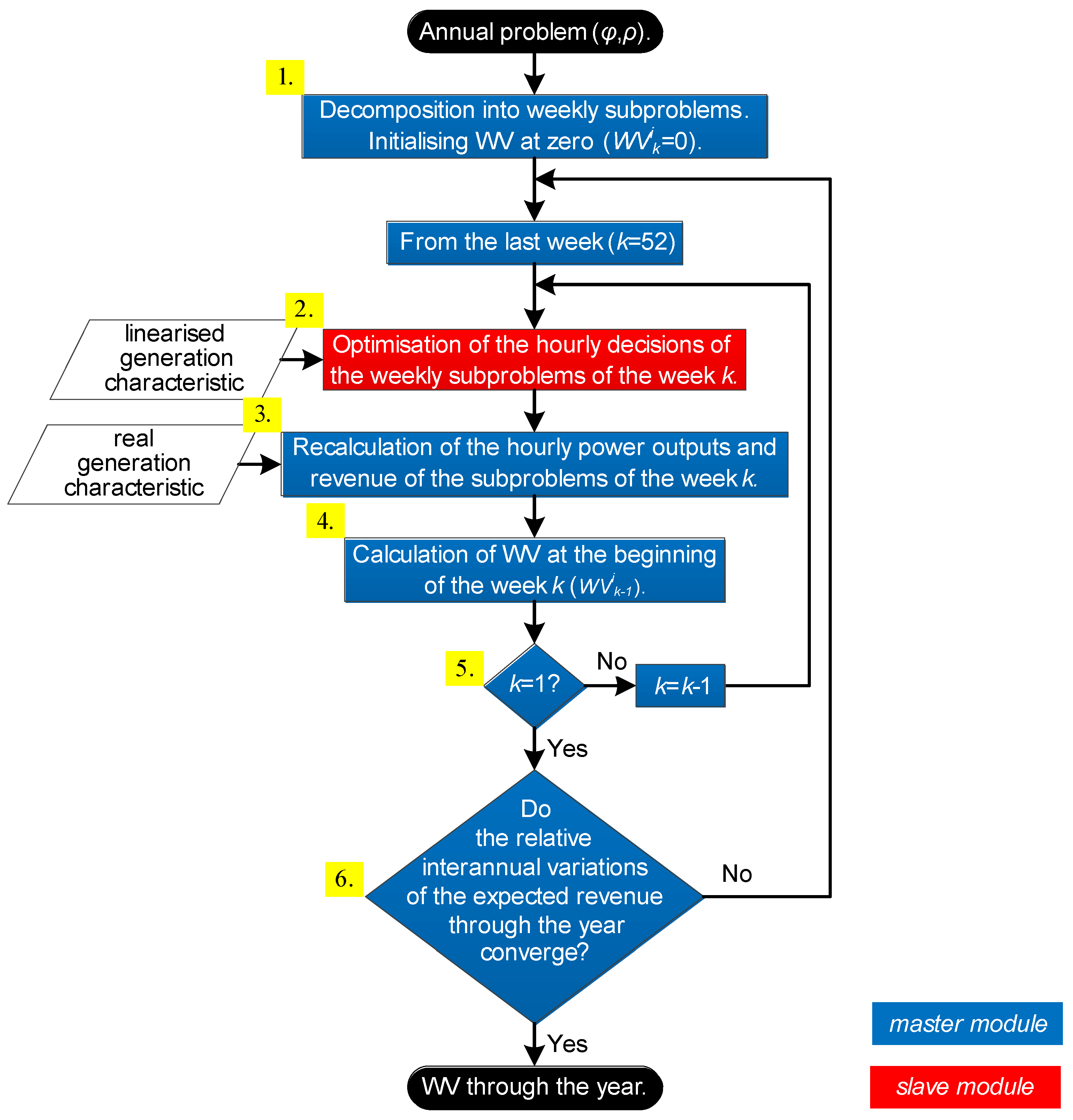
- The master module, based on stochastic dynamic programming (SDP), decomposes the annual scheduling problem, defined by a specific pair of ϕ and ρ, into weekly subproblems.
- The slave module, based on deterministic mixed integer linear programming (DMILP), solves each weekly subproblem in the considered week. The weekly subproblems are aimed at maximizing the weekly revenue plus the future expected revenue (given by WV) from a linearized generation characteristic. The process starts from the last week.
- The master module recalculates, with the real generation characteristic of the plant, the power outputs according to the decisions provided by the slave module and obtains the resulting revenue.
- The master module calculates WV at the beginning of the week.
- Second, third and fourth steps are repeated backwards until the beginning of the year for the rest of the weeks using the last-obtained WV.
- The master module checks if the relative interannual variations of the expected revenue at the beginning of each week converge (see Equation (4)). If the answer is yes, the process stops, otherwise the process is repeated from the second step but now considering the last-obtained WV at the end of the last week.
2.1. Master Module
2.2. Slave Module
- Water mass balance (Equation (6)):This equation is analogous to Equation (2) where means the stored volume at the end of the hour t and T contains the set of hours of the week.
- Initial (Equation (7)), final maximum legal (Equation (8)), hourly maximum physical (Equation (9)) and hourly minimum physical (Equation (10)) stored volume:
- Hourly evaporation losses (Equation (11)):where is a conversion factor for converting m3/s into Mm3/week (1/0.6048), signifies the rate of hourly evaporated water volume per flooded area during the week k, and and are the coefficients of the linear approximation of the storage-flooded area curve of the reservoir.
- Use of the bottom outlets and spillways (Equations (12)–(18)):Equation (12) computes the hourly flow increments, , and decrements, , through the bottom outlets and spillways. Equation (13) limits the maximum water release through the bottom outlets according to the hourly stored volume where and are the coefficients of the linear approximation of the storage-maximum bottom outlet flow curve. Equation (14) is analogous to Equation (13) for the case of the spillways where represents the coefficient of the linear approximation of the storage-maximum spillway flow curve and means the stored volume at the end of the hour t above the spillways minimum level. Equations (15)–(18) are used to calculate where is the stored volume at the end of the hour t below the spillways minimum level, is the stored volume above which the spillways can operate, and indicates whether (1) or not (0) the stored volume is above during the hour t.
- Maximum plant flow according to the stored volume and minimum technical stored volume for power generation (Equations (19)–(21)):Equation (19) is analogous to Equations (13) and (14) for the case of the hydro units where is the length (measured in terms of flow) of the c-th segment of the storage-maximum plant flow curve and indicates whether (1) or not (0) the stored volume is above the minimum storage of the c-th segment during the hour t. It is important to clarify that Equation (19) is added since the maximum plant flow may vary substantially within each week at low reservoir levels. Equations (20) and (21) are used to calculate , where is the length (measured in terms of volume) of the c-th segment of the storage-maximum plant flow curve and indicates whether (1) or not (0) at least one hydro unit is on-line during the hour t.
- Power-discharge piecewise non-concave linear curve as in [35], in terms of the initial and estimated final stored volumes (Equations (22)–(25)):In Equation (22), the first term means the minimum flow of a single hydro unit () and the second one the sum of the flow in all segments () in which the power-discharge curve is divided. Equations (23) and (24) define the maximum and minimum values of each . In Equation (25), the first term signifies the minimum power output of one hydro unit () and the second one refers to the sum of the power in all segments of the power-discharge curve, each calculated as the product of and the slope of each segment ().
- Interhourly variation of the generated power (Equation (26)):Equation (26) computes the interhourly power increments, , and decrements, .
- Equations (27)–(29) are used to calculate the operating state of the hydro units () according to where means the plant flow above which the u-th hydro unit starts up and represents the total number of hydro units of the plant. Equations (30) and (31) compute the changes in the operating state of the hydro units.
- Future expected revenue at the end of the week (Equations (32)–(35)):where is the length (measured in terms of volume) of the j-th segment of the storage-WV curve, is the stored volume in the j-th segment of the said curve at the end of the week, and indicates if the stored volume at the end of the week is above the minimum storage of the j-th segment.
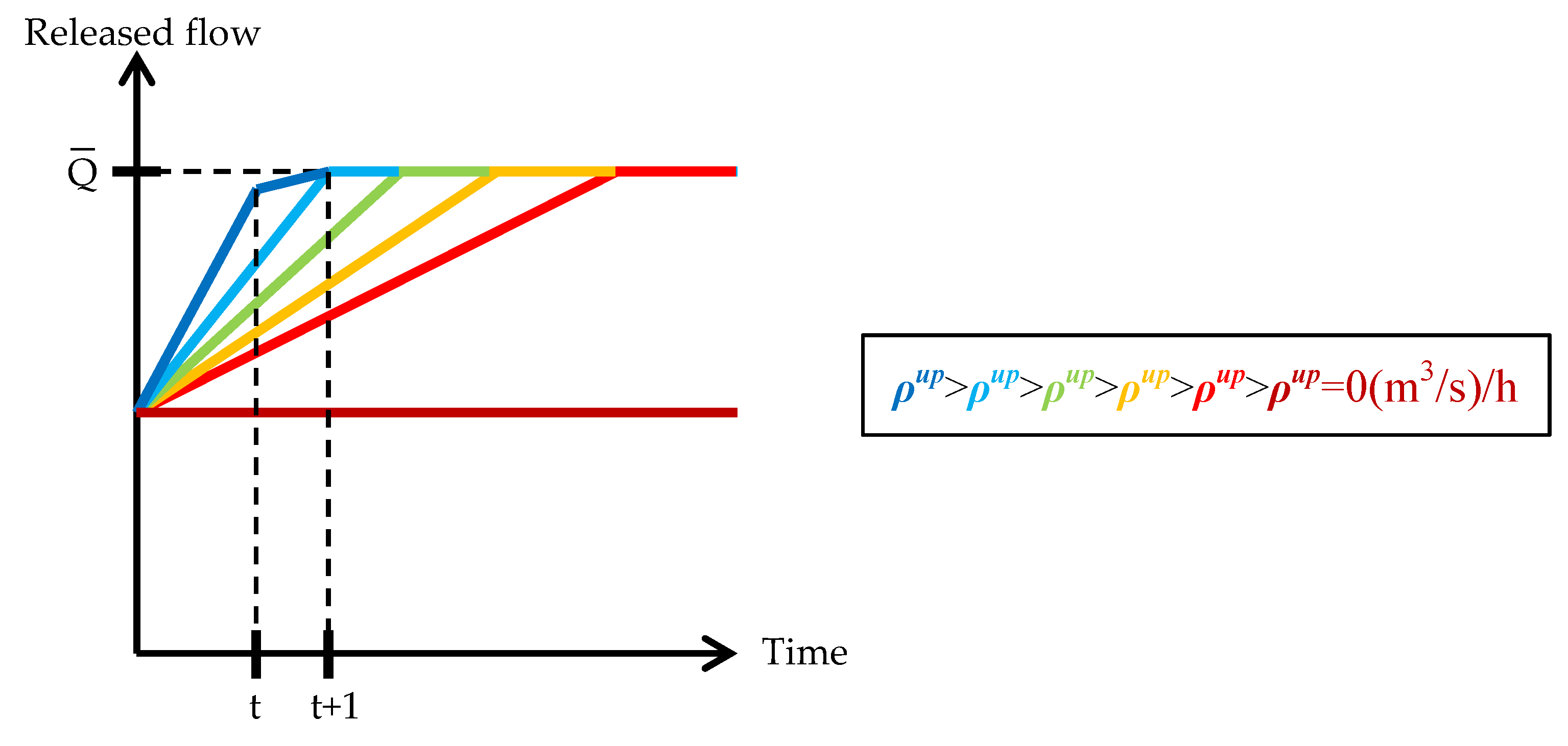
- Up and down ρ as in [37] (Equations (36) and (37)):where and refer to the maximum interhourly increment and decrement of water release, respectively. The fulfillment of ρ between consecutive weeks is not considered and is one of our ongoing works. The interested reader is referred to [38] where the fulfillment of the interweekly ρ was considered in a deterministic context.
- Seasonal ϕ (Equation (38)):Equation (38) forces the total water release (through the hydro units, bottom outlets and spillways) to be larger than or equal to the minimum of ϕ and the current water inflow into the reservoir, [39].
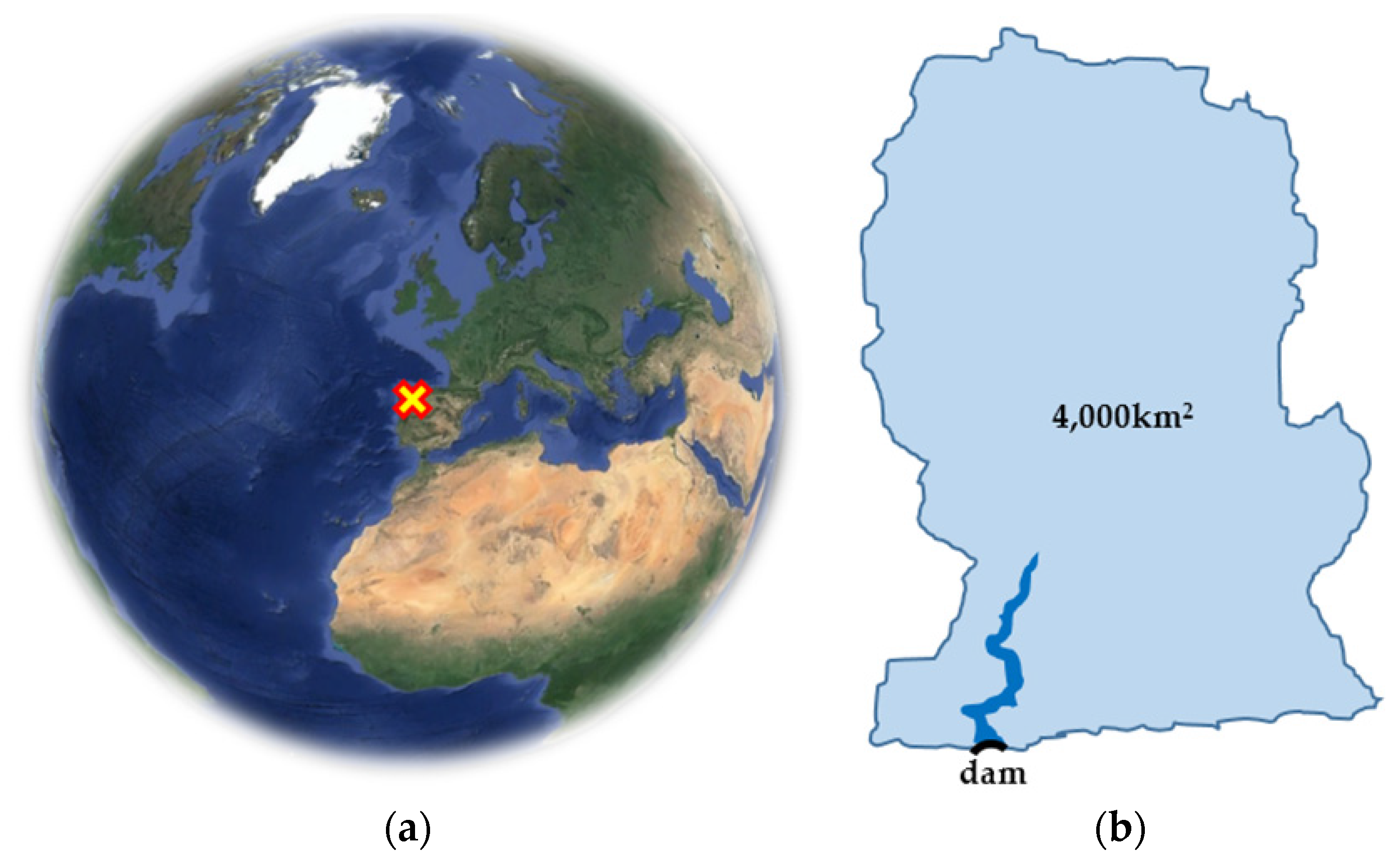
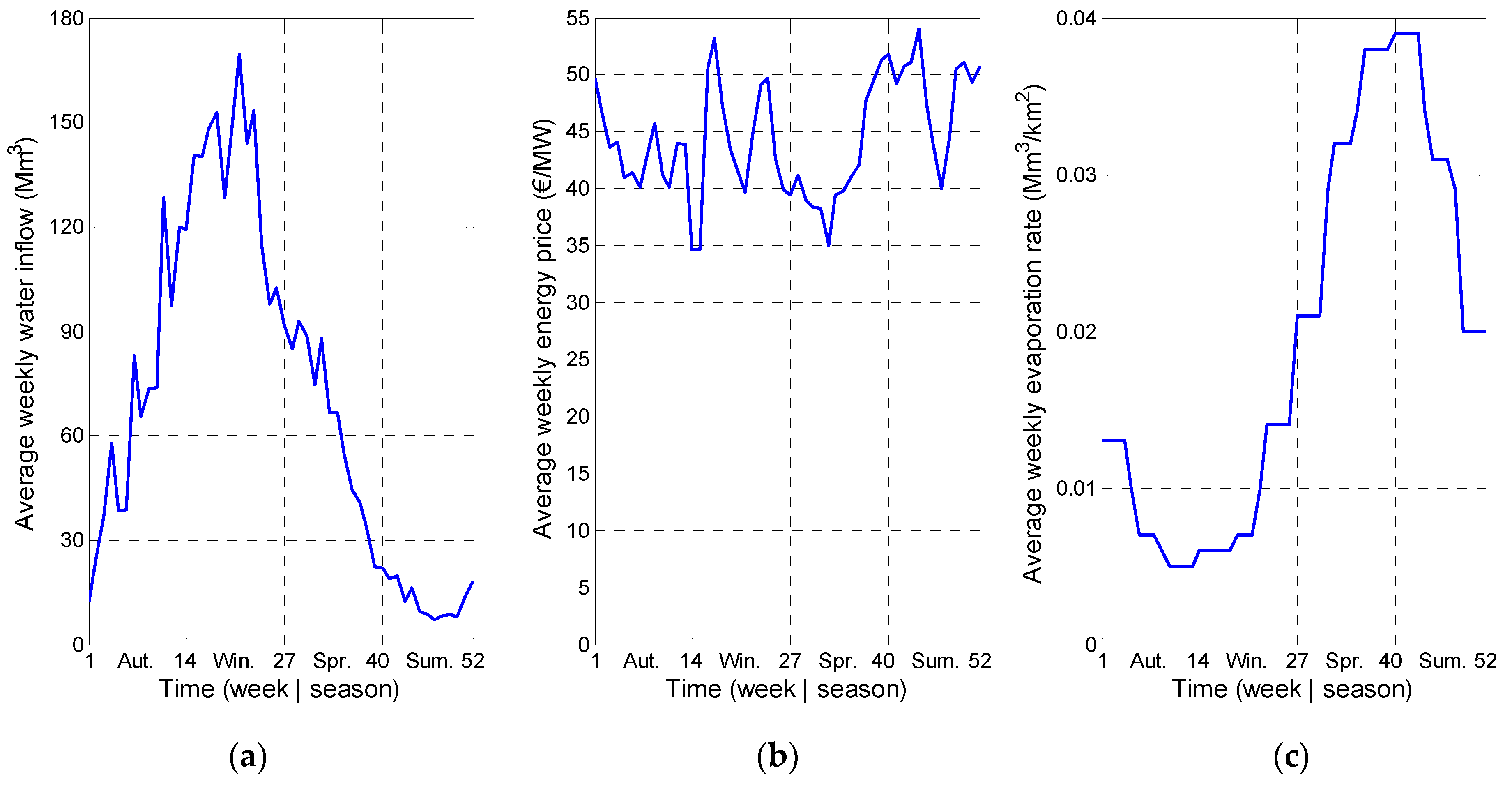
3. Case Study
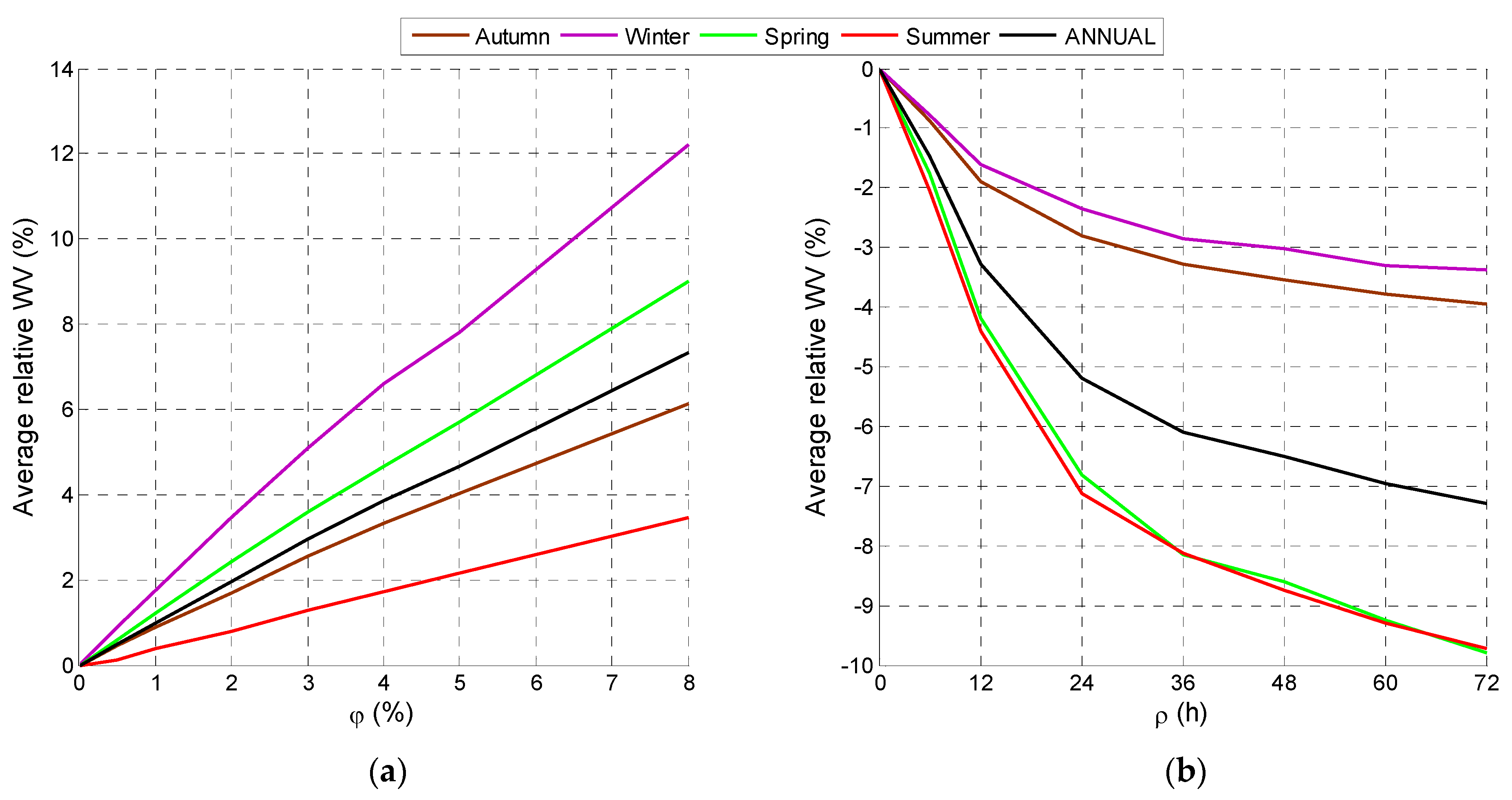
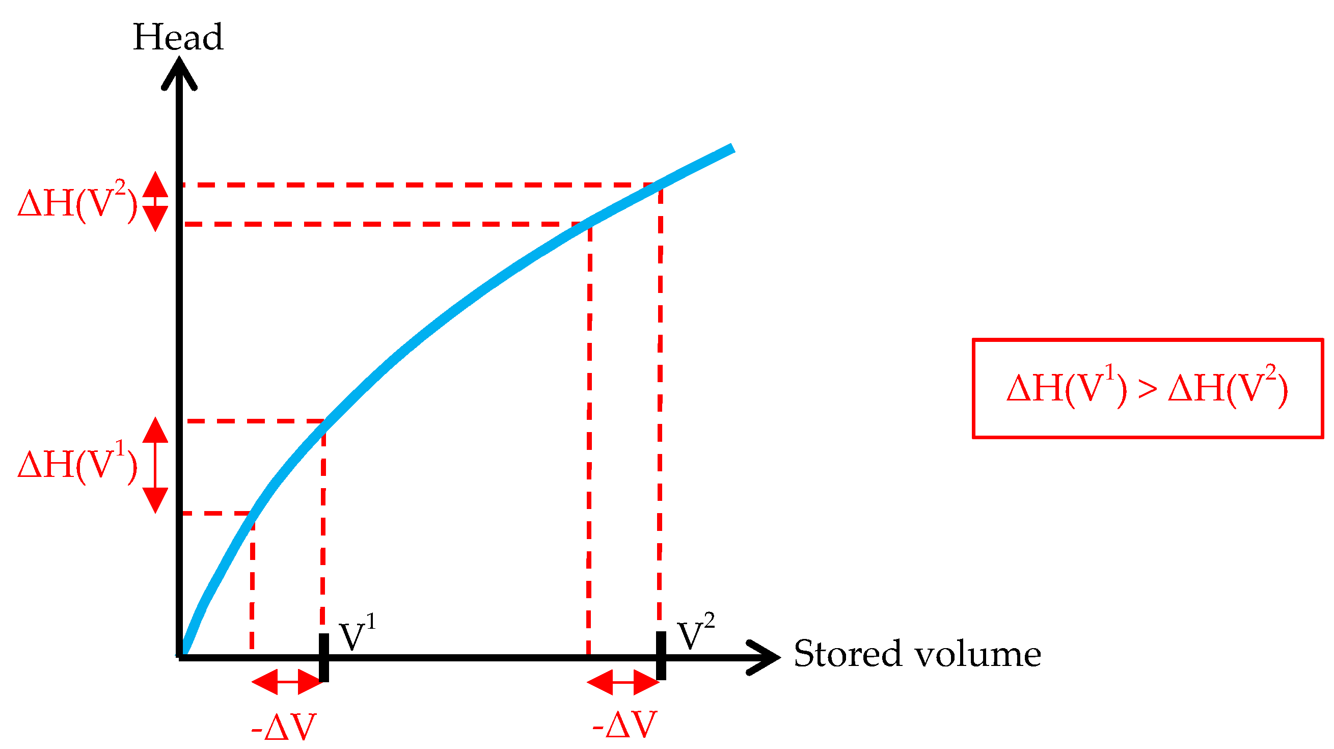
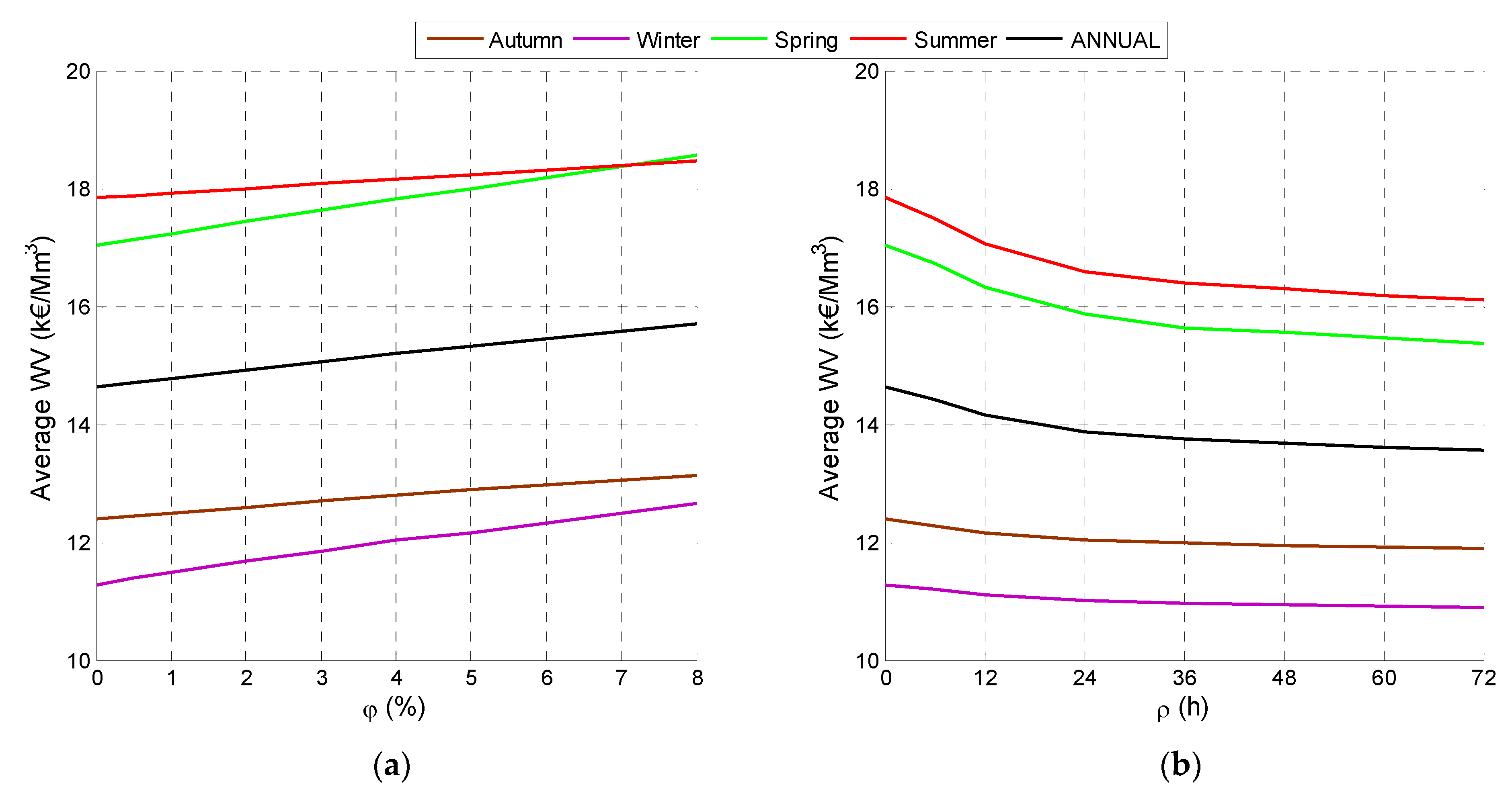
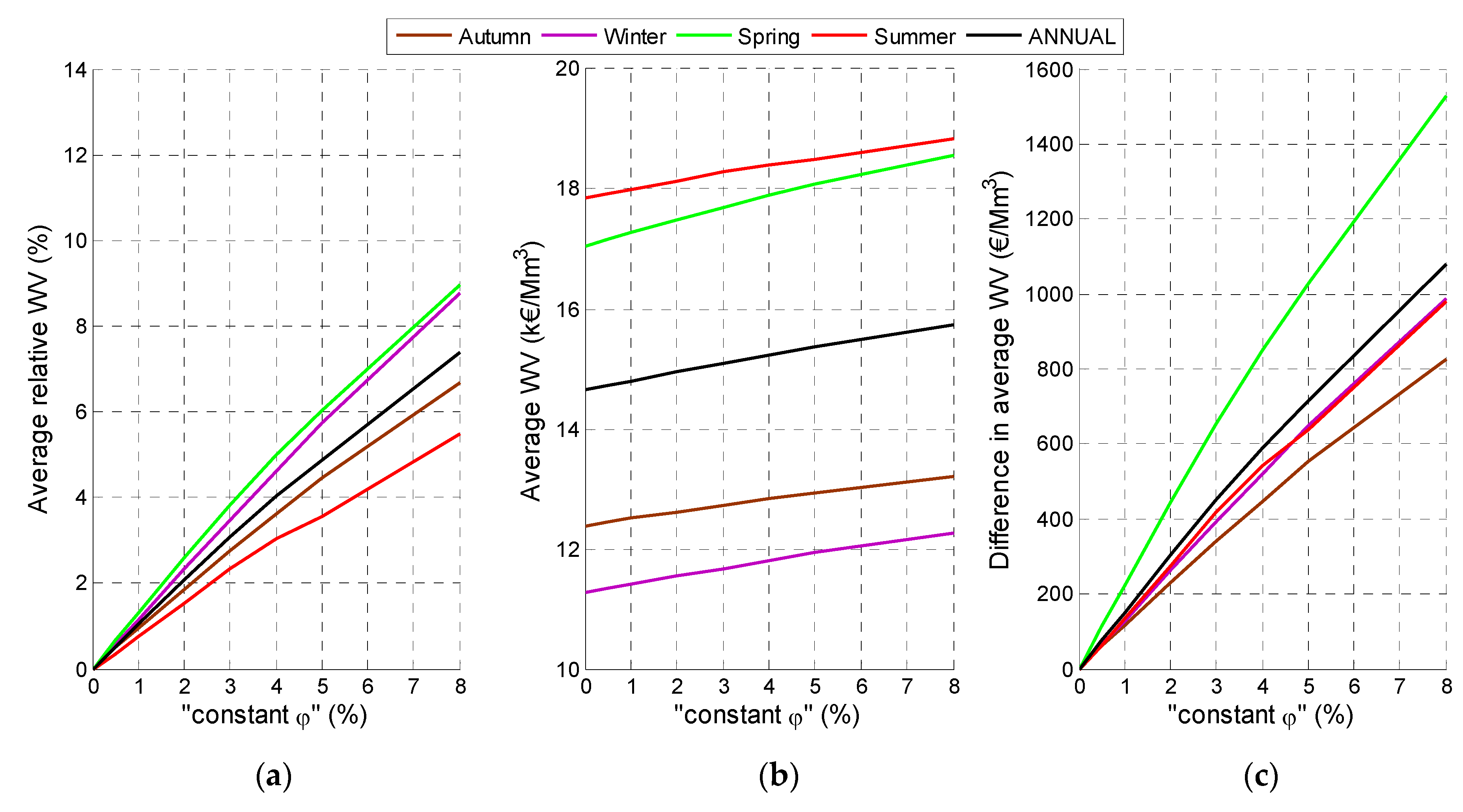
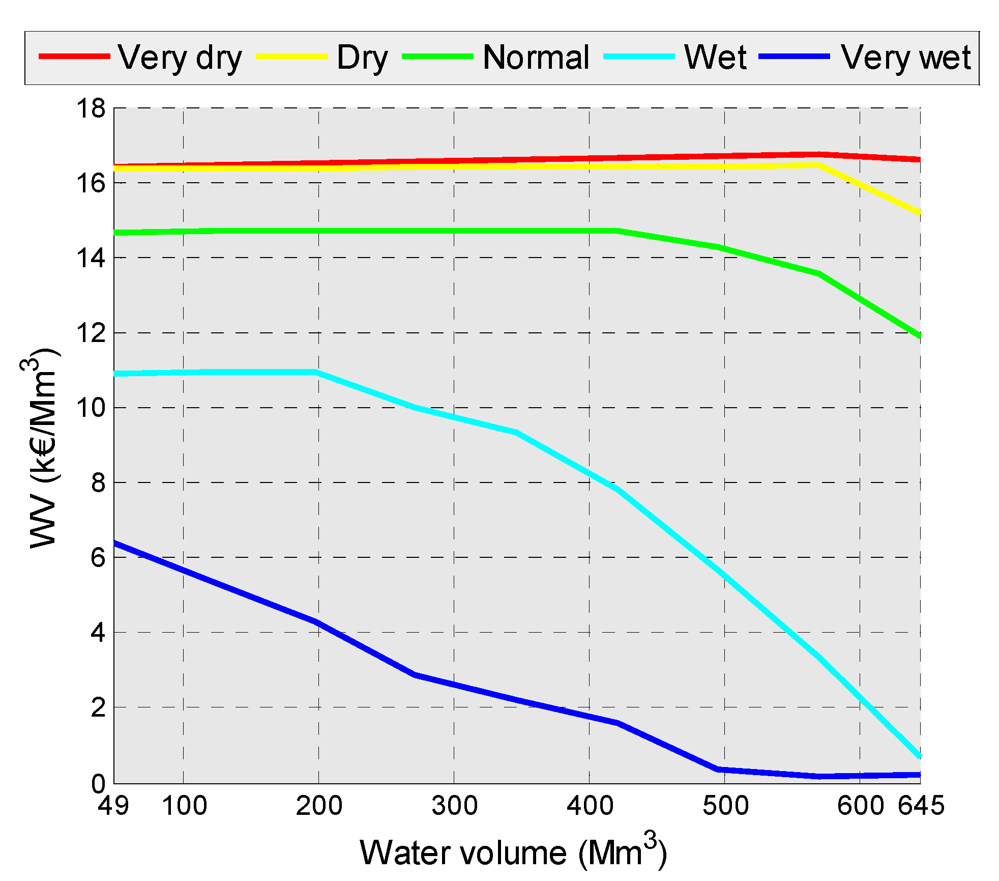
4. Results and Discussion
5. Conclusions
Acknowledgments
Author Contributions
Conflicts of Interest
Abbreviations
| ϕ | Minimum environmental flow(s) (%) |
| ρ | Maximum ramping rate(s) (h) |
| DMILP | Deterministic mixed integer linear programming |
| SDP | Stochastic dynamic programming |
| WV | Water value(s) |
Appendix
| Indexes | |
| a | Weekly water inflow. |
| b | Average weekly energy price. |
| c | Segment of the storage-maximum plant flow curve. |
| i | Initial stored volume. |
| k | Week of the year. |
| l | Final stored volume. |
| n | Iteration of the SPD. |
| j | Segment of the storage-WV curve. |
| s | Segment of the power-discharge curve. |
| su | First segment of the power-discharge curve of the u-th hydro unit in ascending order of flow. |
| t | Hour within the week. |
| u | Hydro unit of the plant. |
| x | Weekly water inflow in the next week. |
| y | Average weekly energy price in the next week. |
| Constants | |
| Conversion factor (0.0036 (Mm3/h)/(m3/s)). | |
| Conversion factor (1/0.6048 (Mm3/week)/(m3/s)). | |
| Parameters | |
| α | Wear and tear costs of hydro units due to variations in the generated power (€/MW). |
| β | Start-up and shut-down costs of hydro units (€/ud). |
| γ | Virtual cost of the bottom outlets and spillways due to variations in the released flow (€/m3/s). |
| Probability that the inflow at the week k +1 is x given that the inflow at the week k was a. | |
| Probability that the average energy price at the week k + 1 is y given that the average energy price at the week k was b. | |
| Rate of hourly evaporated water volume per flooded area during the week k (Mm3/km2). | |
| ϕ during the week k (m3/s). | |
| Total number of segments in the storage-WV curve. | |
| , | Coefficients of the linear approximation of the storage-maximum bottom outlet flow curve ((m3/s)/Mm3; m3/s). |
| , | Coefficients of the linear approximation of the storage-flooded area curve (km2/Mm3; Mm3). |
| Coefficient of the linear approximation of the storage-maximum spillway flow curve ((m3/s)/Mm3). | |
| Down ρ ((m3/s)/h). | |
| Up ρ ((m3/s)/h). | |
| Energy price during the hour t (€/MW). | |
| Minimum power output of the power-discharge curve (MW). | |
| Maximum plant flow (m3/s). | |
| Maximum flow of the s-th segment of the power-discharge curve (m3/s). | |
| Plant flow above which the u-th hydro unit starts up (m3/s). | |
| Plant flow corresponding to the c-th interval of the storage-maximum plant flow curve (m3/s). | |
| Slope of the s-th segment of the power-discharge curve (MW/(m3/s)). | |
| Total number of hydro units of the plant. | |
| Maximum physical stored volume (Mm3). | |
| Dead reservoir volume (stored volume below the bottom outlets) (Mm3). | |
| Stored volume i at the beginning of the week k (Mm3). | |
| Maximum legal stored volume at the end of the week k (Mm3). | |
| Stored volume above which the spillways can operate (Mm3). | |
| Minimum stored volume of the c-th interval of the storage-maximum plant flow curve (Mm3). | |
| Stored volume of the j-th segment of the storage-WV curve (Mm3). | |
| Water inflow to the reservoir during the hour t (m3/s). | |
| WV of the j-th reservoir segment of the storage-WV curve at the end of the week k (€/Mm3). | |
| WV of the j-th reservoir segment of the storage-WV curve at the end of the week k given the inflow a and the average energy price b (€/Mm3). | |
| Sets | |
| C | Intervals of the storage-maximum plant flow curve. |
| J | Segments of the storage-WV curve. |
| K | Weeks of the year. |
| S | Segments of the power-discharge curve. |
| T | Hours of the week. |
| Ω k | Feasible states within the state diagram of the master module during the week k. |
| Binary variables | |
| =1 if the u-th hydro unit is shut-down during the hour t. | |
| =1 if the u-th hydro unit is started-up during the hour t. | |
| =1 if the u-th hydro unit is on-line during the hour t. | |
| =1 if the stored volume is above during the hour t. | |
| =1 if the stored volume is within the c-th interval of the storage-maximum plant flow curve during the hour t. | |
| =1 if the stored volume is above the minimum storage of the j-th segment of the storage-WV curve. | |
| Non-negative variables | |
| Flow of evaporation during the hour t (m3/s). | |
| Lagrange multipliers of the equality constraints during the hour t (€). | |
| Lagrange multipliers of the inequality constraints during the hour t (€). | |
| Generated power during the hour t (MW). | |
| Decrease in generated power between the hours t and t + 1 (MW). | |
| Increase in generated power between the hours t and t + 1 (MW). | |
| Plant flow during the hour t (m3/s). | |
| Plant flow corresponding to the s-th segment of the power-discharge curve during the hour t (m3/s). | |
| Released flow through the bottom outlets during the hour t (m3/s). | |
| Released flow through the spillways during the hour t (m3/s). | |
| Decrease in released flow through the bottom outlets and the spillways between the hours t and t + 1 (m3/s). | |
| Increase in released flow through the bottom outlets and the spillways between the hours t and t + 1 (m3/s). | |
| Stored volume at the end of the hour t (Mm3). | |
| Stored volume at the end of the hour t above the spillways (Mm3). | |
| Stored volume at the end of the hour t below the spillways (Mm3). | |
| Stored volume in the j-th segment of the storage-WV curve at the hour 168 (Mm3). | |
| Revenue corresponding to the decision to go from the stored volume i, inflow a and average energy price b to the stored volume l during the week k (€). | |
| Optimum cumulative revenue at the stored volume i from the week k to the end of the planning period (€). | |
| Optimum cumulative revenue at the stored volume i, inflow a and average energy price b from the week k to the end of the planning period (€). | |
| Optimum cumulative revenue at the stored volume i, inflow a and average energy price b from the week k to the end of the planning period of the iteration n of the SDP (€). | |
| Future expected revenue starting from the volume stored at the final hour of the week (€). | |
References
- Guisández, I.; Pérez-Díaz, J.I.; Wilhelmi, J.R. Influence of the Maximum Flow Ramping Rates on the Water Value. Energy Procedia 2016, 87, 100–107. [Google Scholar] [CrossRef] [Green Version]
- United Nations. The Dublin Statement on Water and Sustainable Development. In Proceedings of the International Conference on Water and the Environment, Dublin, Ireland, 26–31 January 1992.
- Savenije, H.H. Why water is not an ordinary economic good, or why the girl is special. Phys. Chem. Earth Parts A/B/C 2002, 27, 741–744. [Google Scholar] [CrossRef]
- Reneses, J.; Barquín, J.; García-González, J.; Centeno, E. Water value in electricity markets. Int. Trans. Electr. Energy Syst. 2015, 26. [Google Scholar] [CrossRef]
- Fosso, O.B.; Belsnes, M.M. Short-term hydro scheduling in a liberalized power system. In Proceedings of the IEEE International Conference on Power System Technology, Singapore, Singapore, 21–24 November 2004.
- Stage, S.; Larson, Y. Incremental cost of water power. Power Apparatus and Systems, Part III. Trans. Am. Inst. Electr. Eng. 1961, 80, 361–364. [Google Scholar]
- Gebrekiros, Y.; Doorman, G.; Jaehnert, S.; Farahmand, H. Bidding in the frequency restoration reserves (FRR) market for a hydropower unit. In Proceedings of the 4th Innovative Smart Grid Technologies Europe, Copenhagen, Denmark, 6–9 October 2013.
- Perera, K.K.Y.W. A Study of Power System Economic Operation. Ph.D. Thesis, University of British Columbia, Vancouver, BC, Canada, August 1969. [Google Scholar]
- United Nations. Agenda 21. In Proceedings of the United Nations Conference on Environment & Development, Rio de Janeiro, Brazil, 3–14 June 1992.
- British Petroleum. BP Statistical Review of World Energy June 2015. Available online: http://www.bp.com/content/dam/bp/pdf/Energy-economics/statistical-review-2015/bp-statistical-review-of-world-energy-2015-full-report.pdf (accessed on 24 April 2016).
- Cushman, R.M. Review of ecological effects of rapidly varying flows downstream from hydroelectric facilities. N. Am. J. Fish. Manag. 1985, 5, 330–339. [Google Scholar] [CrossRef]
- Dynesius, M.; Nilsson, C. Fragmentation and Flow Regulation of River Systems in the Northern Third of the World. Science 1994, 266, 753–762. [Google Scholar] [CrossRef] [PubMed]
- Richter, B.; Baumgartner, J.; Wigington, R.; Braun, D. How much water does a river need? Freshw. Biol. 1997, 37, 231–249. [Google Scholar] [CrossRef]
- Vörösmarty, C.J.; Sharma, K.P.; Fekete, B.M.; Copeland, A.H.; Holden, J.; Marble, J.; Lough, J.A. The storage and aging of continental runoff in large reservoir systems of the world. Ambio 1997, 26, 210–219. [Google Scholar]
- Clarke, K.D.; Pratt, T.C.; Randall, R.G.; Scruton, D.A.; Smokorowski, K.E. Validation of the Flow Management Pathway: Effects of Altered Flow on Fish Habitat and Fishes Downstream from a Hydropower Dam, Canadian. Available online: http://www.dfo-mpo.gc.ca/Library/332113.pdf (accessed on 24 April 2016).
- Vörösmarty, C.J.; McIntyre, P.B.; Gessner, M.O.; Dudgeon, D.; Prusevich, A.; Green, P.; Glidden, S.; Bunn, S.E.; Sullivan, C.A.; Liermann, C.R.; et al. Global threats to human water security and river biodiversity. Nature 2010, 467, 555–561. [Google Scholar] [CrossRef] [PubMed]
- Young, P.S.; Cech, J.J., Jr.; Thompson, L.C. Hydropower-related pulsed-flow impacts on stream fishes: A brief review, conceptual model, knowledge gaps, and research needs. Rev. Fish Biol. Fish. 2011, 21, 713–731. [Google Scholar] [CrossRef]
- Destouni, G.; Jaramillo, F.; Prieto, C. Hydroclimatic shifts driven by human water use for food and energy production. Nat. Clim. Chang. 2013, 3, 213–217. [Google Scholar] [CrossRef]
- Jaramillo, F.; Destouni, G. Local flow regulation and irrigation raise global human water consumption and footprint. Science 2015, 350, 1248–1251. [Google Scholar] [CrossRef] [PubMed]
- Kosnik, L. Balancing Environmental Protection and Energy Production in the Federal Hydropower Licensing Process. Available online: http://ssrn.com/abstract=1004572 (accessed on 24 April 2016).
- European Commission. Ecological Flows in the Implementation of the Water Framework Directive. Available online: https://circabc.europa.eu/sd/a/4063d635–957b-4b6f-bfd4-b51b0acb2570/Guidance%20No%2031%20-%20Ecological%20flows%20%28final%20version%29.pdf (accessed on 24 April 2016).
- Harpman, D.A. Assessing the short-run economic cost of environmental constraints on hydropower operations at Glen Canyon Dam. Land Econ. 1999, 75, 390–401. [Google Scholar] [CrossRef]
- François, B.; Borga, M.; Anquetin, S.; Creutin, J.D.; Engeland, K.; Favre, A.C.; Hingray, B.; Ramos, M.H.; Raynaud, D.; Renard, B.; et al. Integrating hydropower and intermittent climate-related renewable energies: A call for hydrology. Hydrol. Process. 2014, 28, 5465–5468. [Google Scholar] [CrossRef]
- Abgottspon, H.; Andersson, G. Approach of integrating ancillary services into a medium-term hydro optimization. In Proceedings of the 12th Symposium of Specialists in Electric Operational and Expansion Planning, Rio de Janeiro, Brazil, 20–23 May 2012.
- Loucks, D.P.; van Beek, E. Water Resources Systems Planning and Management. An Introduction to Methods, Models and Applications; United Nations Organization for Education, Science and Culture: Paris, France, 2005. [Google Scholar]
- Goulter, I.C.; Tai, F.K. Practical implications in the use of stochastic dynamic programming for reservoir operation. J. Am. Water Resour. Assoc. 1985, 21, 65–74. [Google Scholar] [CrossRef]
- Little, J.D.C. The use of storage water in a hydroelectric system. Oper. Res. 1955, 3, 187–197. [Google Scholar] [CrossRef]
- Gjelsvik, A.; Belsnes, M.M.; Haugstad, A. An algorithm for stochastic medium-term hydrothermal scheduling under spot price uncertainty. In Proceedings of the 13th Power Systems Computation Conference, Trondheim, Norway, 28 June–2 July 1999.
- Akaike, H. Information theory and an extension of the maximum likelihood principle. In Proceedings of the 2nd International Symposium on Information Theory, Tsahkadsor, Armenia, 2–8 September 1971.
- Nandalal, K.D.W.; Bogardi, J.J. Dynamic Programming Based Operation of Reservoirs. Applicability and Limits; Cambridge University Press: Cambridge, UK, 2007. [Google Scholar]
- Faber, B.A.; Stedinger, J.R. Reservoir optimization using sampling SDP with ensemble streamflow prediction (ESP) forecasts. J. Hydrol. 2001, 249, 113–133. [Google Scholar] [CrossRef]
- Mo, B.; Gjelsvik, A.; Grundt, A.; Kåresen, K. Optimisation of hydropower operation in a liberalised market with focus on price modelling. In Proceedings of the IEEE Power Tech Conference, Porto, Portugal, 10–13 September 2001.
- Electric Power Research Institute. Hydropower Technology Roundup Report: Accommodating Wear and Tear Effects on Hydroelectric Facilities Operating to Provide Ancillary Services: TR-113584-V4; Tech Results: Las Vegas, NV, USA, 2001. [Google Scholar]
- Nilsson, O.; Sjelvgren, D. Hydro unit start-up costs and their impact on the short term scheduling strategies of Swedish power producers. IEEE Trans. Power Syst. 1997, 12, 38–44. [Google Scholar] [CrossRef]
- Conejo, A.J.; Arroyo, J.M.; Contreras, J.; Villamor, F.A. Self-scheduling of a hydro producer in a pool-based electricity market. IEEE Trans. Power Syst. 2002, 17, 1265–1272. [Google Scholar] [CrossRef]
- Arroyo, J.M.; Conejo, A.J. Modeling of start-up and shut-down power trajectories of thermal units. IEEE Trans. Power Syst. 2004, 19, 1562–1568. [Google Scholar] [CrossRef]
- Guan, X.; Svoboda, A.; Li, C. Scheduling hydro power systems with restricted operating zones and discharge ramping constraints. IEEE Trans. Power Syst. 1999, 14, 126–131. [Google Scholar] [CrossRef]
- Guisández, I.; Pérez-Díaz, J.I.; Wilhelmi, J.R. Effects of the maximum flow ramping rates on the long-term operation decisions of a hydropower plant. In Proceedings of the International Conference on Renewable Energies and Power Quality, Córdoba, Spain, 8–10 April 2014.
- Sanguedo Baptista, R.; De Aquino Galeano Massera Da Hora, M. Estimated ecological flow of the Preto River by the wetted perimeter method. Glob. J. Res. Eng. 2013, 13, 9–12. [Google Scholar]
- Centre for Public Works Studies and Experimentation. Available online: http://ceh-flumen64.cedex.es/anuarioaforos/afo/embalse-nombre.asp (accessed on 24 April 2016).
- Iberian Electricity Market Operator. Available online: http://www.omel.es/files/flash/ResultadosMercado.swf (accessed on 24 April 2016).
- Dragoni, W.; Valigi, D. Contributo alla stima dell’evaporazione dalle superfici liquide nell’Italia Centrale. Geol. Romana 1994, 30, 151–158. [Google Scholar]
- Spanish Statistical Office. Available online: http://www.ine.es/inebaseweb/pdfDispacher.do;jsessionid=09739D168C9F3EF056383E89BACE7A07.inebaseweb01?td=183760 (accessed on 24 April 2016).
- Guisández, I.; Pérez-Díaz, J.I.; Wilhelmi, J.R. Assessment of the economic impact of environmental constraints on annual hydropower plant operation. Energy Policy 2013, 61, 1332–1343. [Google Scholar] [CrossRef]
- Luenberger, D.G. Linear and Nonlinear Programming; Springer: Boston, MA, USA, 2003. [Google Scholar]
- Boshier, J.F.; Manning, G.B.; Read, E. Scheduling Releases from New Zealand’s Hydro Reservoirs. Available online: http://search.informit.com.au/documentSummary;dn=428516368419970;res=IELENG (accessed on 7 June 2016).
- Starkey, S.R. Water Allocation under Uncertainty-Potential Gains from Optimisation and Market Mechanisms. Ph.D. Thesis, University of Canterbury, Christchurch, New Zealand, July 2014. [Google Scholar]


| Symbol | Parameter | Value | Unit |
|---|---|---|---|
| Maximum technical storage capacity | 654.1 | Mm3 | |
| Maximum legal storage capacity from 16 April to 14 October | 644.6 | Mm3 | |
| Maximum legal storage capacity from 15 October to 15 April | 607.6 | Mm3 | |
| Volume above which the spillways can operate | 410.6 | Mm3 | |
| Minimum technical volume for power generation | 71.0 | Mm3 | |
| Dead reservoir volume | 48.1 | Mm3 | |
| - | Maximum net head | 132 | m |
| - | Minimum net head | 72 | m |
| Hydro units | 3 | Francis | |
| Maximum plant flow | 279 | m3/s | |
| Minimum hydro unit flow | 40 | m3/s | |
| - | Maximum flow through the bottom outlets | 159 | m3/s |
| - | Maximum flow of the spillways | 2425 | m3/s |
| - | Maximum power output | 312.5 | MW |
| - | Minimum power output | 22.2 | MW |
| Concept | Evaluated Scenarios | Description of Each Scenario |
|---|---|---|
| (ϕ, ρ) | (0.5%, 0 h); (1%, 0 h); (2%, 0 h); (3%, 0 h); (4%, 0 h); (5%, 0 h); (8%, 0 h); (5%, 60 h) 1; (0%, 0 h) 2; (0%, 6 h) 2; (0%, 12 h) 2; (0%, 24 h) 2; (0%, 36 h) 2; (0%, 48 h) 2; (0%, 60 h) 2; (0%, 72 h) 2 | = 0.75ϕ; = 1.75ϕ; = 1.2ϕ; = 0.3ϕ; = 0.75ρ; = 1.5ρ |
© 2016 by the authors; licensee MDPI, Basel, Switzerland. This article is an open access article distributed under the terms and conditions of the Creative Commons Attribution (CC-BY) license (http://creativecommons.org/licenses/by/4.0/).
Share and Cite
Guisández, I.; Pérez-Díaz, J.I.; Wilhelmi, J.R. The Influence of Environmental Constraints on the Water Value. Energies 2016, 9, 446. https://doi.org/10.3390/en9060446
Guisández I, Pérez-Díaz JI, Wilhelmi JR. The Influence of Environmental Constraints on the Water Value. Energies. 2016; 9(6):446. https://doi.org/10.3390/en9060446
Chicago/Turabian StyleGuisández, Ignacio, Juan I. Pérez-Díaz, and José R. Wilhelmi. 2016. "The Influence of Environmental Constraints on the Water Value" Energies 9, no. 6: 446. https://doi.org/10.3390/en9060446