Economic Impacts of Increased U.S. Exports of Natural Gas: An Energy System Perspective

Abstract

With the recent shale gas boom, the U.S. is expected to have very large natural gas resources. In this respect, the key question is would it be better to rely completely on free market resource allocations which would lead to large exports of natural gas or to limit natural gas exports so that more could be used in the U.S.. After accounting for the cost of liquefying the natural gas and shipping it to foreign markets, the current price difference leaves room for considerable profit to producers from exports. In addition, there is a large domestic demand for natural gas from various sectors such as electricity generation, industrial applications, and the transportation sector etc. A hybrid modeling approach has been carried out using our version of the well-known MARket ALlocation (MARKAL)-Macro model to keep bottom-up model richness with macro effects to incorporate price and gross domestic product (GDP) feedbacks. One of the conclusion of this study is that permitting higher natural gas export levels leads to a small reduction in GDP (0.04%–0.17%). Higher exports also increases U.S. greenhouse gas (GHG) emissions and electricity prices (1.1%–7.2%). We also evaluate the impacts of natural gas exports in the presence of a Clean Energy Standard (CES) for electricity. In this case, the GDP impacts are similar, but the electricity and transport sector impacts are different.

1. Introduction

The aim of this study is to examine the likely economic and environmental impacts of increased U.S. exports of natural gas. With the current shale gas boom, the U.S. is expected to have very large natural gas resources. This is true even considering the current low oil and natural gas prices. In recent years, there have been substantial improvements in shale gas technology that have reduced production costs considerably. While it is true that much new drilling ceased when crude oil was around $30/bbl., with oil now above $47/bbl., there are many regions where shale oil and gas plays are becoming attractive again. So the main problem is would it be better to trust solely free market resource allocations which would result in significant level of natural gas exports or to limit natural gas exports so that more could be used in the U.S. Exports would be economically profitable due to the significant price difference at present between U.S. natural gas price (around $3.50/million cubic feet (MCF) in 2010, or $2/MCF in 2016) and prices in foreign markets (e.g., Japanese liquefied natural gas (LNG) Market), which can range up to $15/MCF. After accounting for the cost of liquefying the natural gas and shipping it to foreign markets, price difference leave room for considerable profit from exports. In addition, demand is growing in the electricity, transportation, and industrial sectors. Exporting a large amount of natural gas would definitely increase the natural gas price for all potential domestic uses. Higher natural gas prices would, in turn, mean higher commodity prices coupled with higher energy costs (e.g., electricity prices) for all other sectors that use natural gas. These increased energy prices would also lead to energy intensive sectors to shrink in comparison with the reference case with small natural gas exports. From a global perspective, higher natural gas exports would support the economic interest of foreign companies and hurt domestic energy intensive industries. Besides, foreign consumers also would benefit through lower energy costs, and U.S. consumers would be hurt.

Thus, the problem to be solved is which pathway result in the best economic interest for the U.S. coupled with desirable environmental outcome. This is a very important energy policy question and one difficult to answer because of all the complex economics linkages among different economic sectors and also among the primary energy supply sectors. Our approach is to use a well-established bottom-up energy model named MARKet ALlocation (MARKAL). Use of the term “bottom-up” stands for that the model is built upon thousands of current and future prospective energy technologies and resources. These energy resources supply the projected energy service demands for the sectors that are interest of the economy. Based on the standard MARKAL model, we also have built a version of the MARKAL; MARKAL-Macro model which opens up the possibility to include feedbacks between energy prices and the sectoral economic activities. Through this setup, the impact of alternative energy policies on the gross domestic product (GDP) are captured as well as technology build up and supply use. Since then, MARKAL-Macro is an ideal tool for the current study.

The impacts of different natural gas exports levels on the economy and environment is the main interest of this study. In the reference case, we allow as much as 2.7 billion cubic feet (BCF) /day of natural gas exports level since that level is already permitted, and the other explored cases are complementary of 6, 12, and 18 BCF/day of natural gas exports over current export levels. These levels were chosen based on the Energy Information Administration (EIA) simulated levels [1] and to provide a wide range of natural gas export levels to determine how sensitive the various metrics are to the level. The export levels are compared with a reference case. Current U.S. policy requires Department of Energy (DOE) approval for all natural gas exports, so an important question is to what extent that approval should be granted.

Since the renewable fuels standard (RFS) for biofuels and the corporate average fuel economy (CAFE) standard for automobile and light duty vehicle fuel economy are now established U.S. policy, we have included those policies in the reference case. However, the reality is, for this particular question, the results would not be very different between a reference case with and one without these policies. Our interest is in the difference or delta caused by three levels of increased natural gas exports compared with the reference case. Since current policy is that natural gas cannot be exported without DOE approval, this analysis effectively tests different levels of export approval.

We do also examine one additional policy called the Clean Energy Standard (CES). This is the CES proposed by President Obama in his first term. The CES targets 80% clean energy, doubling the percentage of current clean electricity from 40%, by 2035. Clean electricity includes coal with carbon capture and sequestration, nuclear, solar, hydropower, biomass, and wind. Electricity produced by the combustion/reaction of natural gas based is accepted as 50% clean in the CES. We also developed reference case with CES. We, then compare that with the scenarios with three levels of natural gas exports as well. CES policy is implemented into the model such that the technologies listed above are counted as clean electricity while the other technologies’ production is counted as non-clean electricity. As the final stage of implementation a constraint is added such that ratio of clean electricity production to total (clean and non-clean) production must be greater than or equal to minimum limits stipulated in the CES policy.

The remainder of this paper is divided into four sections. First we provide a short literature review. Then we provide a more complete description of the MARKAL-Macro model used for the analysis. Third we provide the main results of the analysis comparing the three levels of natural gas exports with the reference and reference plus CES cases. Finally, we provide the conclusions we glean from this analysis.

2. Relevant Literature

While there are many papers in the literature that have used MARKAL and some that have used a version of MARKAL-Macro, we will not review that literature. Other papers we have written provide that literature review [2,3,4,5,6,7,8,9,10]. Here, the only directly relevant study is the recently completed National Economic Research Associates (NERA) Economic Consulting study done for the U.S. DOE [11]. They used, NewERA model, which is their own built energy-economy model for the analysis. Their model’s outcome suggest that the U.S. achieves economic gains from natural gas exports and that the gains increase as the level of natural gas exports grows. Their result is the classical economic result that free trade provides net gains to the economy under most conditions. While economic theory does not suggest that free trade always produces economic gains for all parties under all conditions, the general argument is that under a wide range of conditions, positive net benefit in total with some winners and some losers are expected. The NERA results point elevated natural gas prices due to exports with the magnitude of the increase depending on domestic and global supply and demand factors. The input data required and the relevant information used with in the NERA study is supplied from a companion study done by the Energy information Agency in DOE [1], which estimated the impacts of export levels on U.S. natural gas prices.

Main export levels focused for the analysis were 6 and 12 BCF per day by the NERA study, but there were many other alternative scenarios and related sensitivity analyses. Based on various scenario runs, the welfare or net income increases estimated to be ranging from 0.01% to 0.025% compared to business as usual case. Due to higher natural gas prices, significant losses in capital and wage income in various sectors, and income gains to natural gas resource owners through export earnings and wealth transfers to resource owners are observed. By 2030 the net increase in GDP is expected to be about $10 billion 2010 $, which could be sensed as insignificantly small in a $15 trillion economy [12]. Wage income declines in agriculture, energy intensive sectors, and the electricity sector. Most importantly, the percentage declines in income in these sectors were generally much greater than the percentage increases in net national income. Besides, natural gas price with in domestic market did not exceed 20 % in any of the simulations. The NewERA energy-economy model takes inputs from the EIA National Energy Modeling System (NEMS) natural gas projections [1] and from a global natural gas model. The key difference between NewERA and the MARKAL model employed is the price response of the natural gas sector for the shale gas production in U.S. The NewERA model is built upon on the assumption that production of natural gas does not inherit any delayed response, however extraction of natural gas is a function of both investment (number of wells drilled) and the time (dynamics of each drilling site with respect to time) [13,14]. Thus the models expected price responses for the studied export levels can be viewed as optimistic due to not including engineering limitations of the well timing.

3. Modeling Methodology

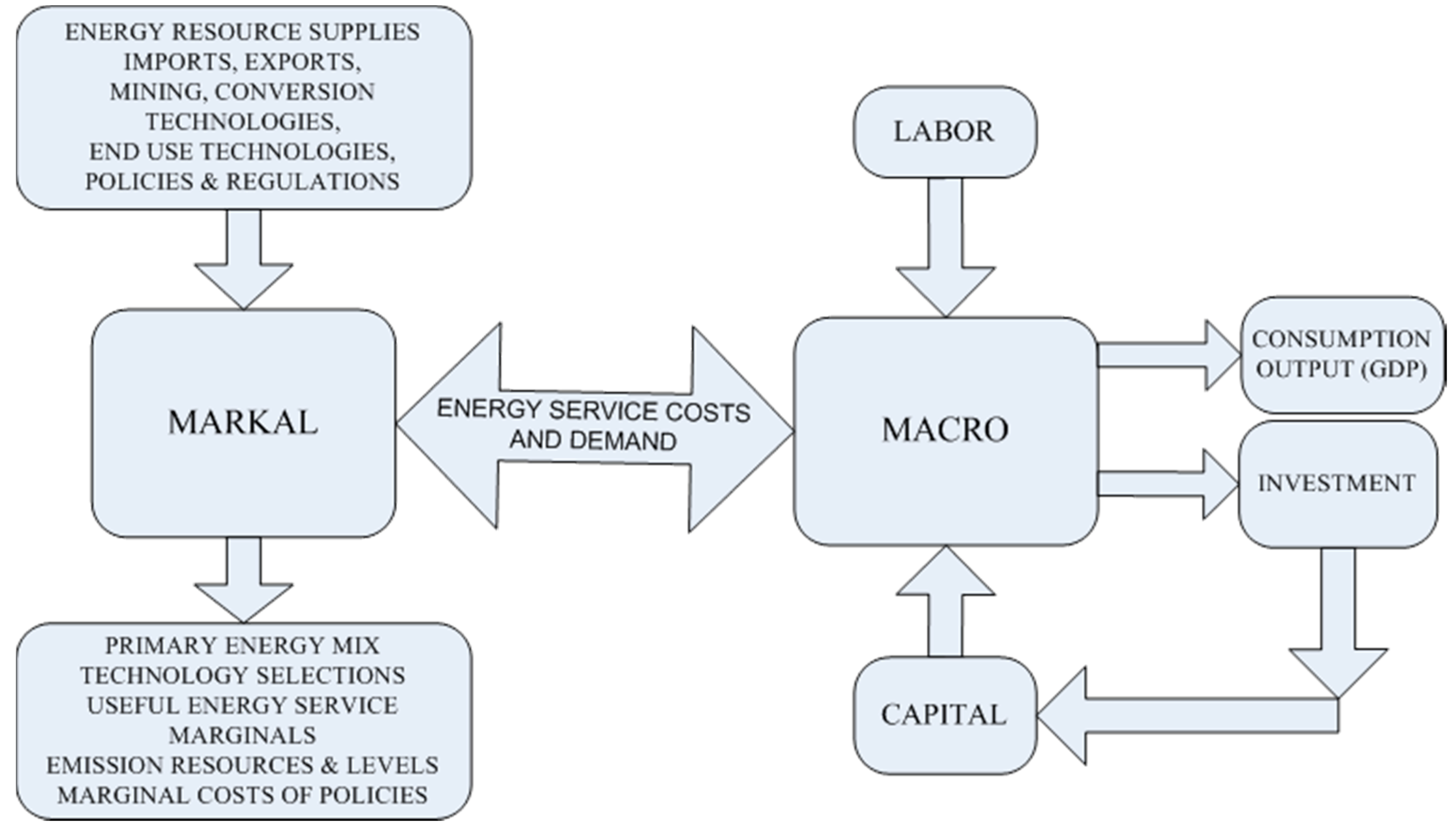
3.1. U.S. MARket ALlocation-Macro Model

MARKAL is a widely applied, dynamic, perfect-foresight, technology-rich linear programming, energy systems, optimization model. In its standard formulation, its objective function is the minimization of the discounted total system cost which is formed by summation of capital, fuel and operating costs for resource, process, infrastructure, conversion and end use technologies. The general framework enables the calibration of a model to local, national, regional or multiregional energy systems. Climate policy, impact assessment of new technologies, taxes, subsidies, and various regulations are frequent model applications. Further details regarding the methodology can be found in Loulou et al. [15].

The U.S. Environmental Protection Agency (EPA) MARKAL is a standard, single region MARKAL model which is linear, has perfect foresight over the planning horizon, and energy service demands are exogenous, and inelastic. A database that represents a particular energy system must be developed to use with MARKAL. The U.S. EPA [16] developed MARKAL databases that represent the U.S. energy system at the national and regional levels. National and regional databases cover the same sectors representing the resource supplies, electricity production, residential, commercial, industrial and transportation sectors for the period 2005 through 2055 in five-year long time steps. The U.S. EPA MARKAL model has been used for several national or international studies [17,18,19]. The original model has now been updated to 2010 data since the relevant data for the modifications in the following sections has been mostly available for the year 2010. In this study we use the national single region U.S. EPA MARKAL model.

Parameter estimation of current and expected future technologies, quantification of energy demands, and resource supplies within the model database were extracted mainly from the Energy Information Agency’s 2010 Annual Energy Outlook report, extrapolated to 2055 using NEMS outputs published by DOE [20]. Additional data sources include the AP-42 emission factors from U.S. EPA [21], and Argonne National Laboratory’s greenhouse gas, regulated emissions, and energy use in transportation (GREET) model [22]. Details regarding U.S. EPA MARKAL database can be reached in Shay et al. [23].

3.2. Model Modifications

Significant data and model changes were introduced into MARKAL for this analysis:

• supply-chain of biomass was introduced including land rents from the global trade analysis project (GTAP) model. Essentially, we captured the land rents as a result of increasing the amounts of specific biofuels demanded in that model and used those land rent responses for constructing land supply curves to be used in MARKAL;
• the biochemical conversion technologies in MARKAL were updated to the latest and most reliable available in the literature at the time of model development;
• biomass thermochemical conversion technologies were added to the model. All these changes are detailed in previous work [24];
• new data on natural gas supply was introduced to reflect the increased supply of shale gas;
• the transportation sector compressed natural gas (CNG) use has been restructured.

Each of these modifications is discussed in greater detail below:

The approach for the modeling of biomass production in the original U.S. EPA MARKAL is similar to the approach used for modeling of conventional energy resource production (e.g., oil, natural gas, coal or hydraulic power production), where the production activity itself does not interfere significantly with any other economic activity. Competition for another resource is minimal due to the production processes of coal, natural gas or uranium. In extreme, you do not have to sacrifice production of oil to produce uranium or vice versa. The real difference is due to the use of land for biomass production itself interferes with the ongoing conventional agricultural activity such as crops, vegetables or any other related agricultural good production. In that sense the current U.S. EPA MARKAL model or any national or international MARKAL model does not reflect this reality.

The introduction of land to the supply chain of corn, corn stover, switchgrass and miscanthus required that a considerable amount of effort to implement both for model modification and data input in the MARKAL modeling framework. The land data came from the Global Trade Analysis Project (GTAP) database. The GTAP land data is stratified into agro-ecological zones (AEZ), so it permitted us to introduce the yield levels by region [25,26]. Land rent data is implemented based on to the GTAP output by the use of piecewise linear approximations. The details regarding this approach can be found in Sarica and Tyner [24]. The total supply chain of the selected biomass products is depicted with the aforementioned changes. Besides the land rent which is now a part of the cost of producing biomass, we have introduced the most up to date seeding, harvesting, transport and harvesting costs for the feedstocks mentioned earlier [25].

Another important change was to update the EPA MARKAL data base natural gas supply curves with improved supply curves from the Massachusetts Institute of Technology (MIT) Energy Initiative report [27]. Natural gas is expected to be available at low cost for the U.S., due to shale gas and other technological improvements. Due to the expectation of improvements in gas extraction techniques, the high availability case is quite plausible as suggested by the MIT Energy Initiative Report [27]. With this expectation we make the use of high availability case supply curve in the modified MARKAL database.

The last set of changes is the restructuring of the CNG use in the transportation sector. The distribution of CNG within the sector is restructured such that it can be tracked based on type of use such as light duty vehicles (LDV), transit buses, school buses, garbage trucks and heavy duty vehicles (HDV). And relevant policies can be modeled and adapted accordingly. Based on the fleet sizes and energy use distribution from Federal Transit Authority’s National Transit Database [28], Institute of Education Sciences’ National Center for Education Statistics [29], Waste and Recycling News magazine’s 2010 Hauling and Disposal Rankings [30] and 2002 Economic Census—Vehicle Inventory and Use Survey [31], database has been updated to reflect the economies of scale in those subsectors. Besides, the cost of CNG stations implemented in the model is based on the study by Johnson [32]. The author developed the Vehicle and infrastructure cash-flow evaluation (VICE) model which shows the economies of scale effect on CNG station design.

Our U.S. MARKAL-Macro model is based on the national U.S. EPA MARKAL model with the modifications described in this section and earlier references. In the first stage of the calibration process, the MARKAL model is calibrated to the base year, 2005, to match the model outputs to the electricity outputs, primary energy use, installed technology capacity and sectoral outputs. After the first phase, MARKAL and Macro modules went through an iterative calibration process which is used to match the projected energy service demands and projected GDP growth rates. Annual Energy Outlook [20] is the principal data resource in all calibration processes.

3.3. Macro Linkage

In this paper, a neoclassical growth model has been integrated to the technology rich representation of the U.S. energy system. In spite of simple of the simple structure, MARKAL-Macro is one of the very few hard-linked hybrid modeling (bottom-up/top-down) approaches [33]. Figure 1 graphically summarizes the integration process.

The objective function of MARKAL-Macro, as can be seen in Equation (1), is the maximization of the discounted log of utility, which is basically derived as the log of consumption, accumulated over all modeling horizon periods (t), with an added terminal value. C_t is consumption; kpvs is the value share of capital in the labor-capital aggregate; kgdp is the initial capital-to-GDP ratio; depr is the annual depreciation of the capital stock; and grow is the expected growth rate of the economy. The discount factor udf_t is accumulated discount rate from year t to 0 and udr_t is the year t’s annual discount rate. ny is the number of years per period:

$$\begin{array}{cc}\hfill Utility=& {\displaystyle {\displaystyle \sum }_{t=1}^{T-1}}(ud{f}_t)(\log C_t)+\frac{(ud{f}_T)(\log C_T)}{1-{(1-ud{r}_T)}^{ny}}\hfill \\ & ud{f}_t={\displaystyle \prod }_{t=0}^{t-1}{\left(1-ud{r}_t\right)}^{ny}\hfill \\ & ud{r}_t=\frac{kpvs}{kgdp}-depr-grow\hfill \end{array}$$

(1)

The output of the economy (Y_t) is composed of consumption, investment and energy costs, as shown in Equation (2), in a single economic sector with perfect foresight. The financial link between MARKAL and Macro module is represented by EC_t.

$$Y_t=C_t+I_t+E{C}_t$$

(2)

where I_t is investment; and EC_t is the total energy cost where a simplified breakdown is given in Equation (3). k stands for utilized technologies in this equation. The key point in Equation (3) is the revenue generated from export activities. Any export activity has a potential to reduce the energy system cost thus creating growth potential for other economic activities. Besides, for this to hold, the cost of extracting exported commodity and extra burden created by the disturbance in the energy system must be less than the revenue generated. A more detailed cost description can be found in Loulou et al. [15].

$$\begin{array}{cc}\hfill E{C}_t=& {\displaystyle {\displaystyle \sum }_k}\{AnnualizedInvestmentCosts\left(t,k\right)\hfill \\ & +FixedOperating\&MaintainingCosts\left(t,k\right)\hfill \\ & +VariableOperating\&MaintainingCosts\left(t,k\right)\}\hfill \\ & +MiningActivityCosts\left(t\right)+TradeRelatedCosts\left(t\right)\hfill \\ & +EnergyImportCosts\left(t\right)-EnergyExportCosts(t)\hfill \\ & +EnviromentalTax(t)\hfill \end{array}$$

(3)

Production roots from three substitutable inputs by a nested CES function. As can be seen in Equation (4), under this formulation, capital and labor substitute directly for one another based on the value share of capital in the labor-capital aggregate (kpvs). Their aggregate is then substituted for a separable energy aggregate. Investment is used to build up the stock of (depreciating) capital, while labor is exogenous:

$$\begin{array}{c}{Y}_t={\left[akl{\left(K_t\right)}^{\mathsf{\rho }\mathsf{\alpha }}{\left(L_t\right)}^{\mathsf{\rho }\left(1-\mathsf{\alpha }\right)}+{\displaystyle {\displaystyle \sum }_{dm}}{b}_{dm}{\left(D_{dm,t}\right)}^{\mathsf{\rho }}\right]}^{\raisebox{1ex}{$1$}\!\left/ \!\raisebox{-1ex}{$\mathsf{\rho }$}\right.}\\ L_t={(1+gro{w}_{t-1})}^{ny}{L}_{t-1},\mathrm{where}{L}_0=1\\ \alpha =kpvs,\mathsf{\rho }=1-\frac{1}{ESUB}\end{array}$$

(4)

where akl is the production function constant, b_dm are the coefficients on demands in the Macro objective function; K_t is the capital stock; L_t is labor; D_dm,t is the demand for energy services of type dm in period t; and ESUB is the elasticity of substitution between the energy and the capital-labor aggregate. Parameters akl and b_dm can be determined using base year statistics, via the following two-step procedure. First, the reference price of energy service dm (price(ref)_dm,t) is equated to the partial derivative of Y_t (GDP), as can be seen in Equation (4), with respect to D_dm, yielding:

$$\frac{\partial Y_t}{\partial D_{dm,t}}={\left(\frac{Y_t}{D_{dm,t}}\right)}^{1-\mathsf{\rho }}{b}_{dm}=price{(ref)}_{dm,t}$$

(5)

thus allowing the computation of b_dm, for all dm. After that, the formulation of the production function (Y_t) in base year is employed to compute akl.

Due to the first order optimality condition for the partial derivative of production with respect to demand, the marginal change in output is equal to the cost of changing that demand. In practice this has two main conclusions. First, different demands will be altered based on the cost of changing that demand. So if it is very expensive to reduce a particular demand, then this will be reduced relatively less; Secondly, it is important to ensure that the marginal output (demand) responses are realistic having smooth (and certainly not zero) shadow prices.

Formation of capital stock (K_t) is endogenous and has its own dynamics as described in Equation (6). An additional equation ensures new capital is provided through investment, accounting for depreciated capital:

$$\begin{array}{c}{K}_{t+1}={(1-depr)}^{ny}{K}_t+(ny/2)\left[{(1-depr)}^{ny}{I}_t+I_{t+1}\right]\\ I_0=\left(gro{w}_0-depr\right)K_0\end{array}$$

(6)

Terminal condition, Equation (7), ensures sufficient investment for replacement and constant growth of capital at all-time intervals:

$$K_t\left(gro{w}_t+depr\right)\le I_t$$

(7)

Finally MARKAL supply activities are linked to Macro demand variables through two equations. The demand levels (D_dm,t) and cost of energy (EC_t) are the links between MARKAL and the Macro module.

Let X_j,t be an activity j of MARKAL supplying energy service demand (dm) proportional to supply_j,dm,t in time t. With the autonomous energy efficiency improvements factor (efficiency of converting physical energy to energy services) aeeifac_dm,t MARKAL supply activities are linked to Macro demand variables. This process is also termed demand decoupling since it permits the model to decouple demands from the linear relationship with GDP e.g., cement industry is projected to squeeze down, while light duty vehicle energy service demand is projected to grow higher than GDP growth rates:

$${\displaystyle \sum }_{j}suppl{y}_{j,dm,t}{X}_{j,t}=aeeifa{c}_{dm,t}{D}_{dm,t}$$

(8)

To transfer the costs from MARKAL to Macro, the link in Equation (9) computes for each activity j and period t the cost, cost_j,t, per unit of activity X_j,t (which is equivalent to Equation (3)) and quadratic penalty terms are introduced to smooth the rate of market penetration of new technologies:

$$\begin{array}{l}{\displaystyle {\displaystyle \sum }_j}cos{t}_{j,t}{X}_{j,t}+c{\displaystyle {\displaystyle \sum }_{tch}}{c}_{tch}XCA{P}_{tch,t}^2=E{C}_t\\ CA{P}_{tch,t+1}=expfCA{P}_{tch,t}+XCA{P}_{tch,t+1}\end{array}$$

(9)

where CAP_tch,t is the capacity of technology tch during period t, and XCAP_tch,t is the capacity installed beyond the capacity expansion factor expf that limits the projected capacity of technology tch in period t due to technological, economical and/or environmental factors.

As can be seen in Equation (4), useful energy services from MARKAL are accumulated to form the energy input composite in the production function of the Macro module. In the Macro module, there exists a competition between investment in energy and investment in the rest of the economy. Economic output is determined based on this outcome, and this information is passed back to MARKAL. Based on the MARKAL and Macro connection described, MARKAL-Macro determines a baseline and resultant dynamic responses for energy services demand, technology preferences, related pollutants (e.g., carbon emissions, particulates, NO_x emission etc.), and GDP (Y_t). Despite the aggregated energy demand linkage to the production activities through a single price ESUB, sub-sectoral energy service demands will react decoupled from aggregated energy demand dependent on the economic impacts of their reductions, in which demand marginals express the magnitude of those impacts.

In summary, MARKAL-Macro, with its described structure, is able to incorporate aggregated energy service demand feedback due to price changes in energy. Since the demand changes are autonomous, some energy service demands may be decoupled from economic growth. By integration of Macro portion; calculation of real GDP, consumption and investment in an explicit manner is possible. As it can be seen in Equation (2), GDP is calculated using the expenditure approach. Overall, detailed energy systems analysis is maintained, without loss compared to MARKAL.

3.4. Model Key Parameters

The U.S. MARKAL-Macro model uses 2000 real U.S. dollars as the financial metric throughout the modeling horizon. GDP growth estimates are 3%, 2.5% and 2.4% for 2010–2020, 2020–2030, 2030–2045 periods respectively in line with annual energy outlook (AEO 2010. Energy service demand changes through the modeling horizon are displayed in

Table 1. Annual growth rates of demand (%) (Source annual energy outlook (AEO) in 2010).

Energy Service Demands	Average Growth
	2010–2020	2020–2030	2030–2045
Commercial
Cooking	1.16%	1.30%	1.23%
Lighting	1.36%	1.27%	1.24%
Miscellaneous use of fuels—Diesel	−0.66%	−0.20%	−0.98%
Miscellaneous use of fuels—Electricity	2.46%	2.22%	2.28%
Miscellaneous use of fuels—Liquefied Petroleum Gas	0.34%	0.40%	0.54%
Miscellaneous use of fuels—Natural gas	0.53%	1.42%	0.98%
Miscellaneous use of fuels—Low Sulphur Residual Fuel Oil	−0.58%	0.13%	0.74%
Office Equipment	1.80%	1.34%	1.80%
Refrigeration	1.36%	1.27%	1.24%
Cooling	2.11%	1.74%	1.48%
Heating	1.06%	1.01%	1.03%
Ventilation	1.36%	1.27%	1.24%
Water heating	1.36%	1.27%	1.24%
Industry
Chemical	0.26%	−0.97%	−0.38%
Food	1.92%	1.61%	1.67%
Primary metals	2.80%	−1.90%	−0.61%
Non-Metallic	2.19%	0.49%	0.59%
Paper	1.33%	0.48%	0.61%
Transport vehicles	0.28%	2.82%	1.93%
Aggregate Non-Manufacturing	−0.09%	−0.51%	−0.22%
Other Sector	2.99%	1.31%	1.65%
Residential
Freezing	1.40%	0.99%	1.14%
Lighting	1.93%	1.42%	1.03%
Refrigeration	1.29%	1.61%	1.30%
Cooling	1.70%	0.58%	0.50%
Heating	1.04%	1.00%	0.80%
Water Heating	0.83%	1.14%	0.74%
Other Appliances—Electricity	1.62%	0.27%	−0.10%
Other Appliances—Natural Gas	0.47%	−0.19%	−0.56%
Transportation
Air	1.61%	0.98%	1.35%
Bus	1.16%	1.09%	1.12%
Truck	1.93%	1.42%	1.34%
High duty vehicle	2.33%	1.82%	1.75%
Light duty vehicle	1.83%	1.83%	0.69%
Offroad diesel	0.16%	0.16%	0.16%
Offroad gasoline	0.18%	0.18%	0.18%
Rail—Freight	1.34%	0.74%	0.63%
Rail passenger	1.52%	1.15%	1.24%
Shipping	1.00%	0.75%	0.67%

. Annual growth rate estimate for the period 2030—2045 is set to be long term historical average growth rate for the U.S.

Parameters regarding the Macro portion of the U.S. MARKAL-Macro model are chosen to best represent the U.S. economy. The ESUB between the energy and labor-capital aggregate is assumed to be 0.4, in line with The energy technology systems analysis program (ETSAP) estimate range, 0.2–0.5 [15]. The initial capital to GDP ratio, kgdp, is 2.4, and the optimal value share of capital in the value added nest, kpvs, is 24% are based on historical economic data for the U.S. Model wide discount rate of 5% real is used for all non-demand related sectors. For end use related technologies, technology specific discount rates are implemented to simulate the consumer’s behavior in purchasing newer technologies.

4. Results

We will report results on GDP, primary resource mix, electricity sector price and generation source changes, transport sector impacts, impacts on selected other sectors, and impacts on domestic GHG emissions. In each case, we will compare the reference case with the three levels of natural gas exports.

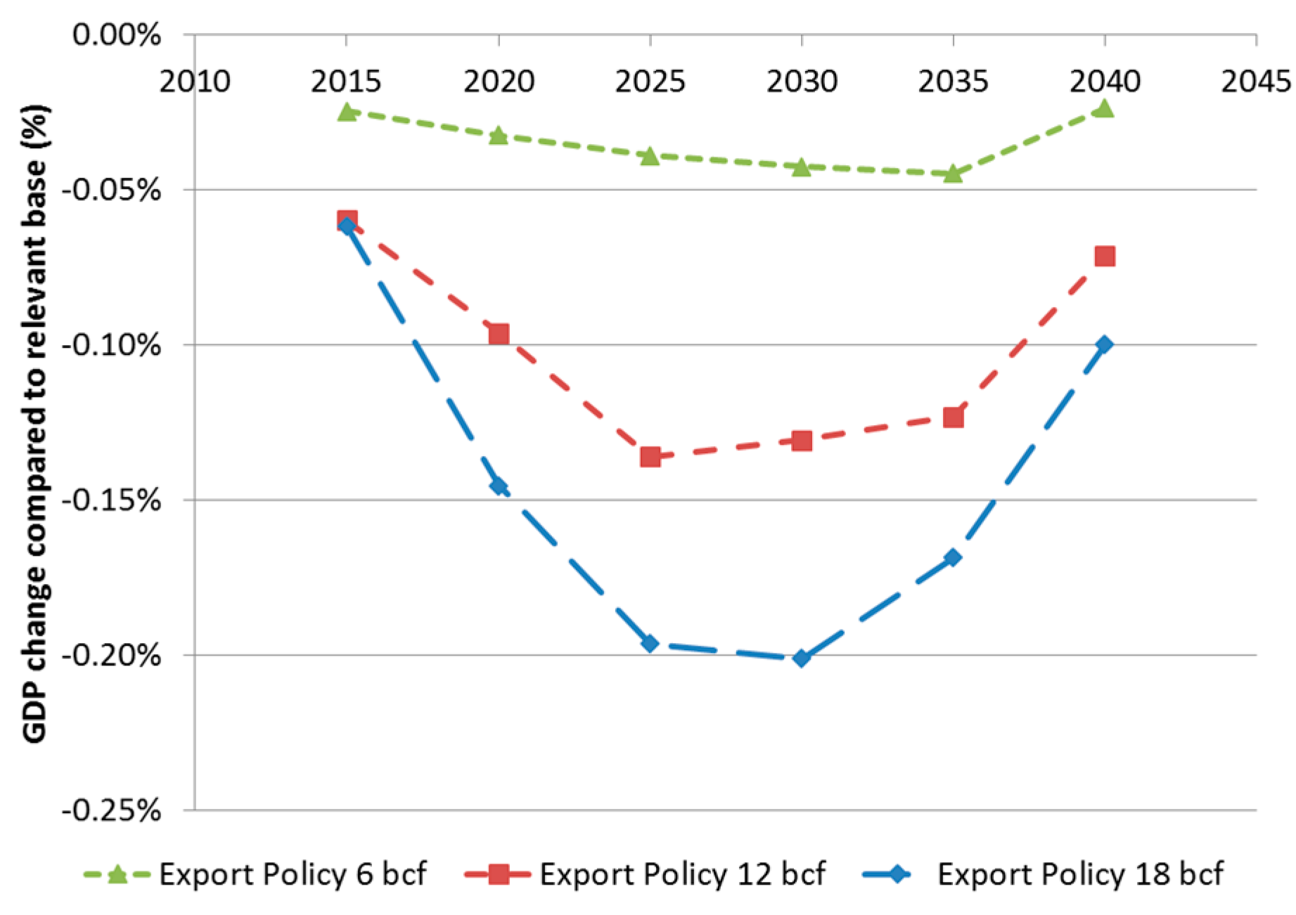
4.1. Gross Domestic Product Impacts

This study shows that increased natural gas exports relative to reference case actually results in a slight decline in GDP. Essentially the gains from exports are less than the losses in electricity and energy intensive sectors in the economy. Figure 2 shows the changes in GDP over time. For the 6, 12, and 18 BCF/day cases, the GDP losses are around 0.04%, 0.11%, and 0.17% respectively relative to reference case for the year 2035. We recognize that this result runs counter to the standard expectation that more open trade results is a net gain for society. However, modern trade theory has many instances of welfare losses to countries and regions from more open trade. Any combination of terms of trade or allocative effects can lead to reduced welfare from more open trade. In any event, the reduction in GDP is relatively small, but it is negative. When we examine the sectoral results below, the sources of the losses will become clearer.

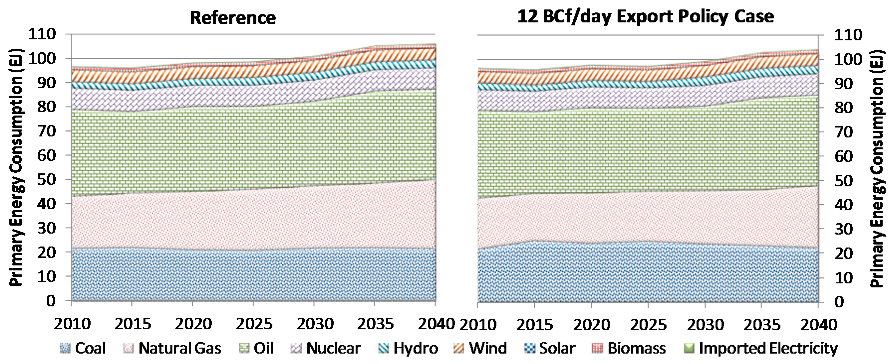
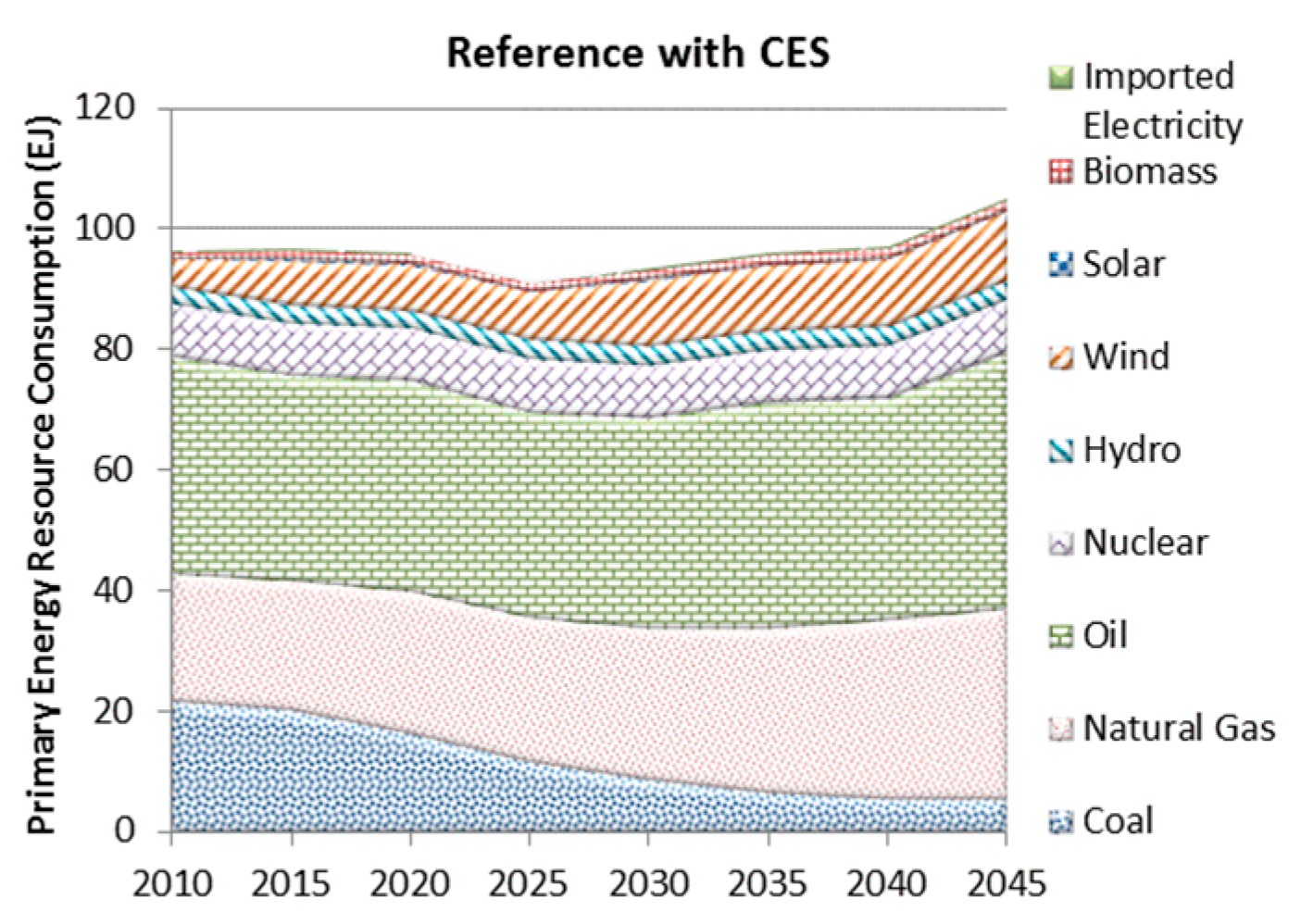
4.2. Energy Resource Mix

The change in energy resource mix with the different levels of natural gas exports for the year 2035 is shown in

Table 2. Energy resource mix for 2035 for the different export cases. BCF: billion cubic feet.

Energy Source	Reference	6 BCF/Day	12 BCF/Day	18 BCF/Day
Coal	20.7%	21.6%	22.3%	22.6%
Natural gas	25.2%	23.8%	22.5%	22.0%
Oil	36.1%	36.4%	36.8%	37.0%
Nuclear	8.3%	8.4%	8.5%	8.5%
Renewables	9.3%	9.4%	9.5%	9.6%
Electricity imports	0.3%	0.3%	0.3%	0.3%

. The relative changes are similar for other years, so we pick 2035 to illustrate the differences among the export levels. The general trends are as follows:

(1)

the domestic energy share for natural gas falls from 25% to 22%;

(2)

domestic use of coal increases from 21% to 23%;

(3)

the fraction of oil in total consumption increases from 36% to 37%;

(4)

there are small increases in nuclear and renewables (hydro, solar, wind, and biomass) as response to increased level of natural gas exports. The directions of all these changes correspond to prior expectations.

Of course, the changes in primary energy mix are driven primarily by the changes in natural gas prices brought on by the increased demand for natural gas for export. Figure 3 shows the percentage changes in natural gas prices over time for the three export cases compared with the reference case. In 2035, natural gas price is 16%, 41%, and 47% higher for the 6, 12, and 18 BCF cases. Post 2035 behavior (drop in price increase) of the prices are mostly related to drop in growth rates for energy service demands due to the long term growth rate projections which can be seen in Table 1. Switch from 2.4% annual growth rate to historical average value diminishes the stress on the domestic gas production by setting lower growth rates targets on the production side compared to previous 5 year periods. These results are higher than the EIA and NERA analysis, and this difference likely is a major driver of the differences in results.

The patterns of primary energy use over time are illustrated in Figure 4, which shows the time profile of primary energy use for the reference and 12 BCF/year cases in terms of absolute units (PJ). Response of the economy to the relevant export policy changes in terms of change in primary energy resource mix is given in Table 2. The patterns evident in Table 2 are clear in Figure 4, but also one can see that the total primary energy consumption is lower in the export case because of the negative impact on GDP.

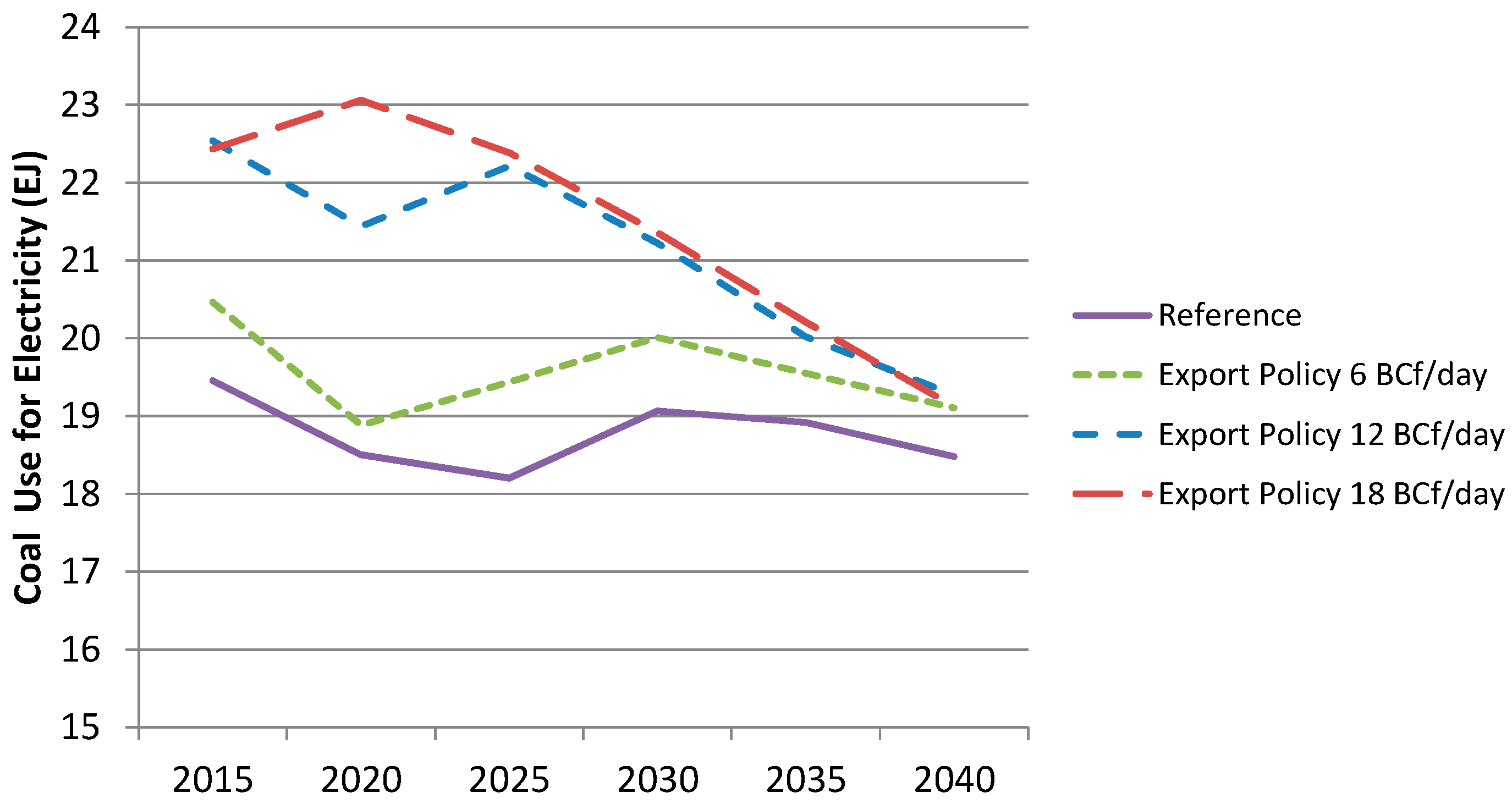
4.3. Electricity Sector Impacts

The impacts on the electricity sector come in higher electricity prices and higher GHG emissions. In 2035, electricity price is up compared with the reference case by 1.1%, 4.3%, and 7.2% for the 6 BCF, 12 BCF, and 18 BCF cases respectively. Of course, these higher electricity prices affect the entire economy through industrial, commercial, and residential sectors electricity consumption.

Electricity GHG emissions in the early years of the simulation horizon are around 2% higher for the 6 BCF case, and 7%–12% higher for the 12 BCF and 18 BCF cases. However, by the end of the simulation period, the differences are all in the 1%–4% range. This decline in emission difference is due to the emergence of less expensive renewable energy technology after 2020 and to some increase in nuclear. The increase in coal use shown in Table 2 exists, but the higher coal emissions relative to natural gas in later years are partially offset by lower emissions from nuclear and renewables. Coal use for electricity generation for the four cases is shown in Figure 5. In the early years, higher natural gas exports results in substantially higher coal use for electricity generation.

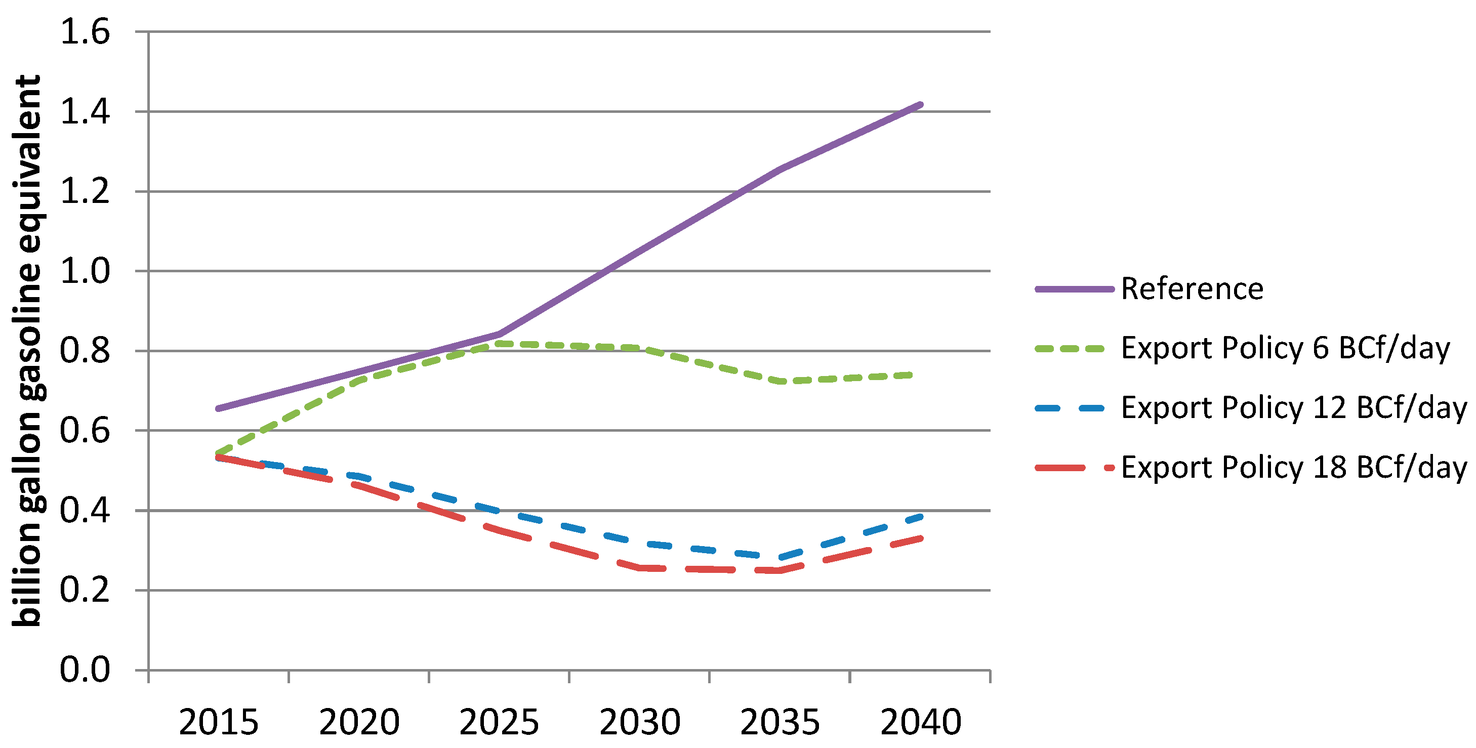
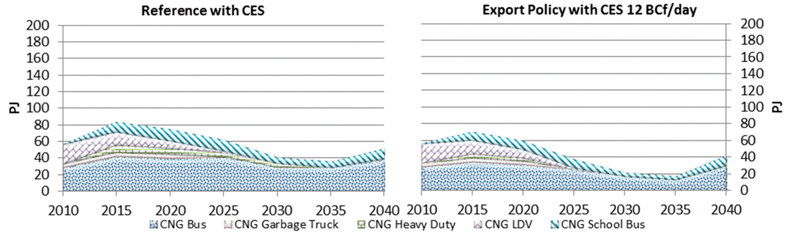
4.4. Transport Sector

Figure 6 shows the CNG use in transportation over time for the reference and three export cases. In 2035, 1.3 billon gallon gasoline equivalent CNG is used in transportation sector, but it drops to 0.2–0.3 range in the three export cases. Figure 7 shows what happens over time to fleet use of natural gas in the reference and 12 BCF cases. CNG use in HDVs disappears in the 12 BCF and 18 BCF case, and CNG use in transportation sector drops considerably. The main result is that even though CNG use in transport is not large in the reference case, it becomes insignificant in the export cases.

4.5. Other Sectors

Examination of impacts on certain sectors of the economy, particularly energy intensive sectors provides insight on why our analysis shows declines in GDP from the natural gas exports and associated higher natural gas prices.

Table 3. Declines in total energy use relative to reference case in 2035 for four important sectors.

Sector	Primary Metals	Non-Metallic	Paper	Chemical
6 BCF/day	−1.4%	−2.2%	−0.8%	−1.8%
12 BCF/day	−3.0%	−3.1%	−2.0%	−2.4%
18 BCF/day	−4.0%	−3.5%	−2.8%	−3.8%

provides the decline in total energy use in four important sectors of the economy for 2035. In every case, total energy use and therefore total sector output declines. The declines are less pronounced for the paper sector, which uses some renewable energy from wood.

4.6. Results with Clean Energy Standard Included in Reference Case

The Clean Energy Standard policy was designed to increase the share of electricity from renewable, nuclear and natural gas based power plants in the electricity sector. It substantially reduces GHG emissions in the electricity sector. Essentially, the sector goes from being 40% to becoming 80% clean by 2035. In all our results natural gas (considered 50% clean) plays a large role in meeting the CES. A policy very similar to the one modeled here has been promulgated by the Obama administration.

The biggest impact of the CES is substantially higher natural gas prices, as natural gas achieves significant penetration in the electric power sector. Thus, it is useful, first, to compare natural gas prices with and without the CES before moving to evaluating impacts of different levels of natural gas exports. Figure 8 shows the absolute price levels over time for the previous reference case and the reference with CES added. In every period, natural gas price is substantially higher under the CES than the standard reference. For example, in 2030, the reference price is $7.02, and the reference with CES is $10.60. Thus, the added demand for natural gas for electricity leads to much higher natural gas price even before considering exports.

Of course if we add exports, the price increases are even higher as illustrated in Figure 9, which shows the percentage increase in natural gas price with 12 BCF/day of exports for both the CES and standard reference cases, both compared with the standard reference. The bottom line is that the CES leads to relatively high natural gas price increases, which are accentuated by natural gas exports.

The GDP impacts of this policy case are pretty comparable with the cases described above. For example, the GDP reductions that were −0.10%–−0.15% for the standard reference are in the same range for the reference with CES. The sectoral impacts also were similar to the standard reference described above.

The primary energy source mix is quite different for the standard reference and reference with CES as would be expected. In the standard reference, coal use was relatively flat over the time horizon, and it increased with increasing natural gas exports. With the reference plus CES, coal use drops drastically (Figure 10) as would be expected since the CES cannot be met with so much coal power in the mix. Compare this primary resource mix with that shown in Figure 4 for the reference case.

Finally, we examine the impacts on the use of CNG in the transport sector. The CES virtually eliminates the use of CNG or LNG in the heavy duty truck sub-sector as shown in Figure 11. Compare this fleet mix (left panel of Figure 11 with the left panel of Figure 7. The right panel of Figure 11 shows the transportation fleets using CNG for the 12 BCF/day export level. It is clear that the combination of CES plus exports causes a huge reduction in CNG use in transportation in the U.S.

5. Conclusions

This study used an energy sector perspective with links to the broader economy for the analysis of possible U.S. LNG export policies. The MARKAL-Macro model, captures the effects of the possible policy options through primary energy resource availability. Changes in the availability of natural gas for the domestic market are signaled through natural gas prices. These price signals affect the domestic use of primary energy sources and the energy service demand through changes in their respective prices. Thus, natural gas demand in various sectors may be reduced according to their respective production mixes. As long as the export prices cover this price response by increasing the income of households, the reduction of the economy coupled with the demand reduction for natural gas intensive sectors may be insignificant or turn out to be positive. However, the quantity of natural gas to be exported is partially independent. Setting a high export level can have a negative effect over the economy, and that is what we see at higher levels. This study explores those possibilities for three possible export permits.

One of the main conclusions of this study is that permitting higher natural gas export levels leads to a small reduction in GDP (0.04%–0.17%) and also increases GHG emissions and other environmental emissions such as particulates. There is loss of labor and capital income in all energy intensive sectors, and electricity prices increase (1.1%–7.2%). The main reason that drives the difference is that we get higher increases in U.S. natural gas that obtained in the NERA analysis. Also, we do not get export revenue high enough to overcome the negative effects of exports in the national economy. The higher natural gas prices cause general losses through wages and income throughout the commercial, industrial, and residential sectors. Interestingly, if global and U.S. crude oil and gas prices did remain low, the lower natural gas production would strengthen further our conclusion that caution is in order in substantially increasing exports. If massive exports were permitted with tight domestic supplies, the domestic price impacts would be even more severe.

We also evaluate the impacts of natural gas exports in the presence of a Clean Energy Standard for electricity. In this case, the GDP and sectoral impacts are similar, but the impacts on electricity and transport are substantially different. The CES induces considerably higher natural gas prices because of the added demand for natural gas for power generation. Natural gas exports on top of CES cause prices to go even higher. In transport, the CES eliminates use of CNG or LNG for heavy duty trucks, and natural gas exports reduce CNG fleets substantially more in addition.

Beyond the analysis conducted here, it is important to note that neither the model used in this analysis nor the NERA model are global in scope. Thus, neither includes the trade impacts of U.S. natural gas exports or GHG emissions on a global scale. However, we can describe those impacts qualitatively. Increased U.S. natural gas exports will reduce energy costs for industry and consumers in foreign countries and increase those costs for the U.S. Thus, U.S. industry will be rendered less competitive compared with foreign industry. This loss of export revenue would be in addition to the GDP loss estimated in this analysis. Moreover, U.S. consumers lose due to higher energy prices, and foreign consumers gain. GHG emissions outside the U.S. may decline to the extent that exported LNG replaces coal based energy generation. However, there may be reverse effects such that lower energy price due to higher availability of LNG may result in cancelling of renewable energy projects.

Given all the results of this analysis, it is clear that policy makers need to be very careful in approving U.S. natural gas exports. Even though, we are supporters of the free trade orthodoxy, one must examine the evidence in each case. We have done that, and the analysis shows that this case is different. Using the natural gas in the U.S. may be more advantageous than exports on a national scale, both economically and environmentally [34].

References

1. Energy Information Administration. Effect of Increased Natural Gas Exports on Domestic Energy Markets; U.S. Department of Energy: Washington, DC, USA, 2012.
2. Kypreos, S. Assessment of CO2 reduction policies for Switzerland. Int. J. Glob. Energy Issues 1999, 12, 233–243. [Google Scholar] [CrossRef]
3. Morris, S.C.; Goldstein, G.A.; Fthenakis, V.M. NEMS and MARKAL-Macro models for energy-environmental-economic analysis: A comparison of the electricity and carbon reduction projections. Environ. Model. Assess. 2002, 7, 207–216. [Google Scholar] [CrossRef]
4. Morales, K.E.L.S.-R. Response from a MARKAL technology model to the EMF scenario assumptions. Energy Econ. 2004, 26, 655–674. [Google Scholar] [CrossRef]
5. Chen, W. The costs of mitigating carbon emissions in China: Findings from China MARKAL-Macro modeling. Energy Policy 2005, 33, 885–896. [Google Scholar] [CrossRef]
6. Chen, W.; Wu, Z.; He, J.; Gao, P.; Xu, S. Carbon emission control strategies for China: A comparative study with partial and general equilibrium versions of the China MARKAL model. Energy 2007, 32, 59–72. [Google Scholar] [CrossRef]
7. Contaldi, M.; Gracceva, F.; Tosato, G. Evaluation of green-certificates policies using the MARKAL-Macro-Italy model. Energy Policy 2007, 35, 797–808. [Google Scholar] [CrossRef]
8. Strachan, N.; Kannan, R. Hybrid modelling of long-term carbon reduction scenarios for the UK. Energy Econ. 2008, 30, 2947–2963. [Google Scholar] [CrossRef]
9. Strachan, N.; Pye, S.; Kannan, R. The iterative contribution and relevance of modelling to UK energy policy. Energy Policy 2009, 37, 850–860. [Google Scholar] [CrossRef]
10. Ko, F.-K.; Huang, C.-B.; Tseng, P.-Y.; Lin, C.-H.; Zheng, B.-Y.; Chiu, H.-M. Long-term CO2 emissions reduction target and scenarios of power sector in Taiwan. Energy Policy 2010, 38, 288–300. [Google Scholar] [CrossRef]
11. NERA Economic Consulting. Macroeconomic Impacts of LNG Exports from the United States; National Economic Research Associates: Washington, DC, USA, 2012. [Google Scholar]
12. Trading Economics. Available online: http://www.tradingeconomics.com/united-states/gdp (accessed on 1 January 2014).
13. Gülen, G.; Browning, J.; Ikonnikova, S.; Tinker, S.W. Well economics across ten tiers in low and high Btu (British thermal unit) areas, Barnett Shale, Texas. Energy 2013, 60, 302–315. [Google Scholar] [CrossRef]
14. Weijermars, R. US shale gas production outlook based on well roll-out rate scenarios. Appl. Energy 2014, 124, 283–297. [Google Scholar] [CrossRef]
15. Loulou, R.; Goldstein, G.; Noble, K. Documentation for the MARKAL Family of Models. Available online: http://www.etsap.org (accessed on 1 January 2014).
16. Johnson, T.L.; DeCarolis, J.F.; Shay, C.L.; Loughlin, D.H.; Gage, C.L.; Vijay, S. MARKAL Scenario Analysis of Technology Options for the Electric Sector: The Impact on Air Quality; U.S. Environmental Protection Agency: Washington, DC, USA, 2006.
17. Sauthoff, A.; Meier, P.; Holloway, T. Assessment of Biodiesel Scenarios for Midwest Freight Transport Emission Reduction; CFIRE 02-10; National Center for Freight and Infrastructure Research and Education: Madison, WI, USA, 2010. [Google Scholar]
18. Schafer, A.; Jacoby, H. Vehicle technology under CO2 constraint: A general equilibrium analysis. Energy Policy 2006, 34, 975–985. [Google Scholar] [CrossRef]
19. Hu, M.; Hobbs, B. Analysis of multi-pollutant policies for the US power sector under technology and policy uncertainty using MARKAL. Energy 2010, 35, 5430–5442. [Google Scholar] [CrossRef]
20. Department of Energy, U.S. Annual Energy Outlook 2010 with Projections to 2035; U.S. Department of Energy, Energy Information Administrator, Office of Integrated Analysis and Forecasting: Washington, DC, USA, 2010.
21. Duprey, R.L. Compilation of Air Pollutant Emission Factors; U.S. Environmental Protection Agency, Office of Air Quality Planning and Standards: Raleigh, NC, USA, 1995.
22. Burnham, A.; Wang, M.; Wu, Y. Development and Applications of GREET 2.7—The Transportation Vehicle-Cycle Model; Argonne National Laboratory, Energy Systems Division: Argonne, France, 2006. [Google Scholar]
23. Shay, C.; DeCarolis, J.; Loughlin, D.; Gage, C.; Yeh, S.; Vijay, S.; Wright, E.L. EPA U.S. National MARKAL Database Documentation; EPA-600/R-06/057; EPA: Washington, DC, USA, 2006. [Google Scholar]
24. Sarica, K.; Tyner, W.E. Analysis of US renewable fuels policies using a Modified MARKAL model. Renew. Energy 2013, 50, 701–709. [Google Scholar] [CrossRef]
25. Taheripour, F.; Tyner, W.E. Global Land Use Changes and Consequent CO2 Emissions due to US Cellulosic Biofuel Program: A Preliminary Analysis; Purdue University: West Lafayette, IN, USA, 2011. [Google Scholar]
26. Tyner, W.E.; Taheripour, F.; Zhuang, Q.; Birur, D.; Baldos, U. Land Use Changes and Consequent CO2 Emissions Due to US Corn Ethanol Production: A Comprehensive Analysis; Purdue University Department of Agricultural Economics: West Lafayette, IN, USA, 2011. [Google Scholar]
27. The MIT Energy Initiative. The Future of Natural Gas—An Interdisciplinary MIT Study; MIT: Cambridge, MA, USA, 2011; Volume 2011. [Google Scholar]
28. Department of Transportation, U.S. Available online: http://www.ntdprogram.gov/ntdprogram/pubs/dt/2011/excel/DataTables.htm (accessed on 31 December 2013).
29. Department of Education, U.S. Available online: http://nces.ed.gov/ccd/elsi/tableGenerator.aspx (accessed on 1 February 2014).
30. Waste and Recycling News. Available online: http://www.wasterecyclingnews.com/article/99999999/DATA/307199975/hauling-disposal-ranking-2010 (accessed on 1 June 2013).
31. Department of Commerce, U.S. 2002 Economic Census—Vehicle Inventory and Use Survey; EC02TV-US; US Census Bureau: Washington, DC, USA, 2004.
32. Johnson, C. Business Case for Compressed Natural Gas in Municipal Fleets; NREL/TP-7A2-47919; National Renewable Energy Laboratory: Washington, DC, USA, 2010.
33. Messner, S.; Schrattenholzer, L. MESSAGE-Macro: Linking an energy supply model with a macro economic model and solving itinteractively. Energy 2000, 25, 267–282. [Google Scholar] [CrossRef]
34. Gillingham, K.; Palmer, K. Bridging the Energy Efficiency Gap: Insights for Policy from Economic Theory and Empirical Analysis; Oxford University Press: Oxford, UK, 2013. [Google Scholar]
Figure 1. MARket ALlocation (MARKAL)-Macro integration.
Energies 09 00401 g001
Figure 2. The changes in gross domestic product (GDP) over time in relevant scenarios compared to reference.
Energies 09 00401 g002
Figure 3. Price change wellhead natural gas price with respect to the reference as percentage.
Energies 09 00401 g003
Figure 4. Primary energy mix for the 12 BCF/day export policy case and the reference scenario.
Energies 09 00401 g004
Figure 5. Coal use for electricity generation.
Energies 09 00401 g005
Figure 6. The compressed natural gas (CNG) use in transportation over time for the reference and three export cases.
Energies 09 00401 g006
Figure 7. The CNG use breakdown in the transportation sector for the 12 BCF/day export policy case and the reference scenario.
Energies 09 00401 g007
Figure 8. Wellhead natural gas prices. CES: clean energy standard.
Energies 09 00401 g008
Figure 9. Natural gas price change comparison for 12 BCF/day policy.
Energies 09 00401 g009
Figure 10. Primary energy mix for the Reference with CES policy.
Energies 09 00401 g010
Figure 11. CNG use breakdown under selected policies.
Energies 09 00401 g011