The Misselhorn Cycle: Batch-Evaporation Process for Efficient Low-Temperature Waste Heat Recovery ^†

Abstract

The concept of the Misselhorn cycle is introduced as a power cycle that aims for efficient waste heat recovery of temperature sources below 100 °C. The basic idea shows advantages over a standard Organic Rankine Cycle (ORC) in overall efficiency and utilization of the heat source. The main characteristic of this cycle is the use of at least three parallel batch evaporators instead of continuous heat exchangers. The operational phases of the evaporators are shifted so that there is always one vaporizer in discharge mode. A transient MATLAB^® model (The MathWorks: Natick, MA, USA) is used to simulate the achievable performance of the Misselhorn cycle. The calculations of the thermodynamic states of the system are based on the heat flux, the equations for energy conservation and the equations of state found in the NIST Standard Reference Database 23 (Reference Fluid Thermodynamic and Transport Properties - REFPROP, National Institute of Standards and Technology: Gaithersburg, MD, USA). In the isochoric batch evaporation, the pressure and the corresponding boiling temperature rise over time. With a gradually increasing boiling temperature, no pinch point limitation occurs. Furthermore, the heat source medium is passed through the evaporators in serial order to obtain a quasi-counter flow setup. It could be shown that these features offer the possibility to gain both high thermal efficiencies and an enhanced utilization of the heat source at the same time. A basic model with a fixed estimated heat transfer coefficient promises a possible system exergy efficiency of 44.4%, which is an increase of over 60% compared to a basic ORC with a system exergy efficiency of only 26.8%.

1. Introduction

Worldwide rising energy demands and growing international environmental awareness cause new challenges for the energy market. As the conventional fossil fuels are more and more controversially discussed, renewable energy sources and the improvement in efficiency both gain in importance. Much research is already made in using renewable energy sources in geothermal, biomass, wind and solar thermal power plants. While solar and wind energy are subject to high fluctuations, geothermal energy is continuous, but strongly depends on the temperature and quality of the water reservoir. Another environmentally-sustainable approach is the conversion of surplus thermal energy from industry and power generation, which is not used yet. Using waste heat from industrial processes or excess heat from gas turbines and engines to generate electrical power would improve the overall efficiency of these applications and save resources. The common basis of all of these thermal energy sources is the relative low to medium temperature level they can offer. A modern steam cycle in a power plant is operated at temperatures up to 600 °C [1]. Changing the working fluid to an organic medium, known as the Organic Rankine Cycle (ORC), can allow temperatures down to 100 °C to be utilized, but the efficiencies are always lower in these ranges. Numerous studies about the general feasibility and the performance of ORCs for low-temperature applications can be found [2,3,4]. The most discussed topics are the working fluid selection [5,6], the ideal cycle parameters [7] and different cycle designs [8,9,10].

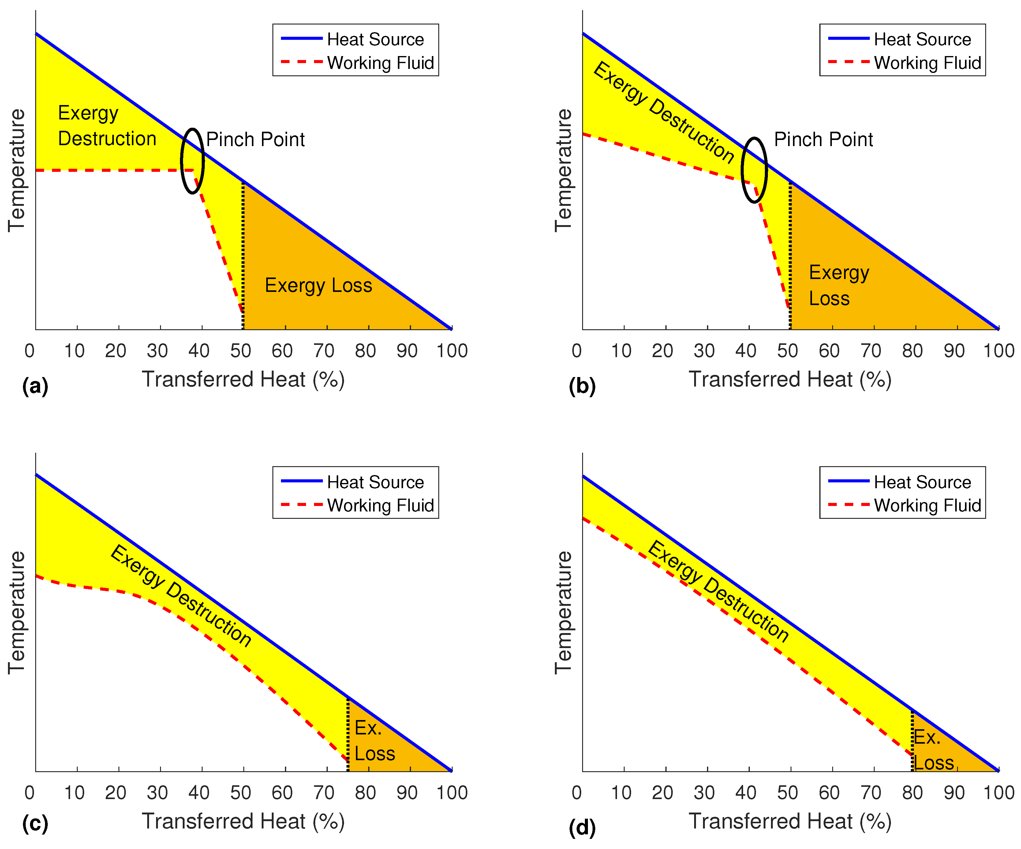
The major reasons for the weak performance at low temperatures are the irreversible losses in the heat exchangers due to temperature differences between the heat source and the working fluid [11]. While the liquid heat source medium is cooling down with a nearly constant slope, the evaporation of the working fluid consists of different parts. The heating of the sub-cooled working fluid also shows a nearly linear profile, whereas the evaporation itself happens at a constant temperature. To keep a reasonable heat exchanger area, the temperature difference between the two fluids has to be bigger than a certain value, normally 5 to 10 K, at every position. Therefore, the possibility to match the two temperatures is limited by the occurring pinch point, as shown in Figure 1a.

The best method to rate the efficiency of a process depends strongly on the given application. In this context, an often used property is the exergy $\mathit{Ex}$. It describes the maximum usable work that can theoretically be created from a heat source with respect to a given dead state. For a common power cycle with a closed heating circuit, the most important parameter is the efficiency of converting the heat that is actually added. This depends on the available vapor pressure, the efficiency of the turbine and on the heat transfer itself. If heat is transferred from a high grade heat source to a lower temperature working fluid, exergy is destroyed (compare Figure 1a). In contrast, many waste heat recovery applications have an open heating circuit where any unused heat is discarded and lost. This unused exergy accounts for the exergy loss. Therefore, the goal is to achieve a combination of a high utilization of the heat source, a good temperature match and an acceptable conversion efficiency.

There are several concepts to reduce the exergy destruction and losses. As shown in Figure 1b, the boiling temperature of a mixture of different fluids will rise during the evaporation [8], as the low boiling component will vaporize first, and the high boiling part will accumulate in the residue.

Another method is the operation close to critical conditions. Especially in transcritical and supercritical cycles, there is no distinction between fluid and vapor phases. Without the temperature plateau during the phase change, the temperature match can be improved [9], as shown in Figure 1c. A disadvantage of this process is the challenging design of the turbine that has to deal with a supercritical working fluid.

Flash cycles focus on single-phase liquid-liquid heat exchange to avoid the pinch point limitation completely. With suitable mass flows, the temperature difference can be equally small over the entire heat exchanger (Figure 1d). The power generation can then either be performed in a two-phase expander [10] or, as in the organic flash cycle [12], the saturated liquid is flash evaporated and the vapor expanded in a common turbine. While the former one still depends on the ongoing two-phase exchanger research, the latter one has to deal with major exergy losses in the throttling valve or an alternative with a more complex process setup [13].

The thermodynamic fundamentals of the Misselhorn cycle were first introduce in [14]. A more viable process setup, as suggested in [15], already combines two of the main objectives of the current state of the cycle. The working fluid is vaporized in a closed batch evaporation. Due to the isochoric phase change, the saturation temperature rises with the ongoing process; the constant temperature phase can be avoided; and a closer match to the heat source temperature can be achieved. In addition, the pressure is completely generated by the isochoric evaporation. Therefore, the power consumption of the feed pump can be considerably reduced. In this paper, an additional cascaded dynamic heat source flow through several heat exchangers in series is introduced. This setup ensures the ideal assignment of temperature levels of the heat source to the corresponding evaporation phases. Transient MATLAB simulations are conducted to analyze the thermodynamic possibilities of this power cycle and to compare it to a common ORC.

2. Description and Analysis of the Misselhorn Cycle

2.1. Basic Concept of the Misselhorn Cycle

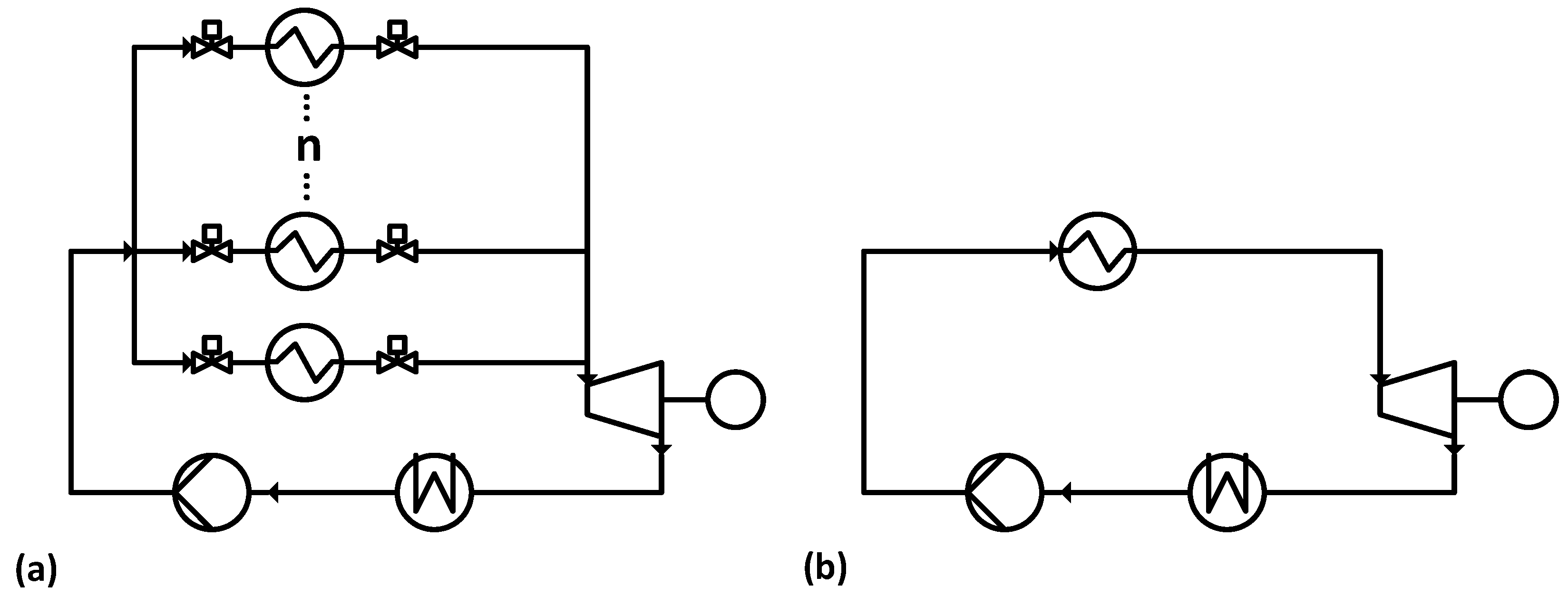
The basic setup of the Misselhorn cycle, as shown in Figure 2a, is similar to a common ORC (Figure 2b). A liquid organic working fluid is evaporated in a heat exchanger, expanded in an expansion engine and condensed in another heat exchanger. The major difference is the non-continuous mode of operation and the pressure levels in the Misselhorn cycle.

In the first phase, the working fluid is pumped into a heat exchanger at condenser pressure. In the second phase, the evaporator inlet and outlet valves are both closed, and the working fluid is at least partly vaporized. Due to the isochoric process, both the pressure and the corresponding boiling temperature of the working fluid rise. Once a certain pressure is reached, the outlet valve is opened, and the vapor flows into the expansion engine (Phase 3). After a defined time, the operating phases are switched again, and the now almost empty vaporizer is refilled. To provide a continuous steam flow, at least three parallel heat exchangers are needed. They are run with shifted phases so that there is always one evaporator in the discharging phase. Regarding the fluctuating vapor outlet parameters, a modified diesel engine is chosen over a turbine as the expansion engine. In this basic setup [15], the heat source flow is split and runs through all heat exchangers in parallel.

2.2. Methods of Analysis

The following efficiencies are defined as the basis for the further analysis and discussions. The most commonly-used efficiency to characterize a power cycle is the thermal efficiency

$${\eta }_{\mathrm{therm}}=\frac{P_{\mathrm{output}}}{{\dot{Q}}_{\mathrm{in}}}$$

(1)

It is defined by the ratio of the power output of the expansion engine $P_{\mathrm{output}}$ versus the actually added heat flow to the cycle ${\dot{Q}}_{\mathrm{in}}$. This contains no information about the utilization of the heat source, but only about the performance of the cycle itself. If heat that is not transferred will still be used in further processes or cogeneration, this efficiency can be useful.

In practice, the maximum work that can be gained from a given heat source with respect to the limitations of the second law of thermodynamics is called the exergy. The specific exergy is generally defined as

$$\mathit{ex}=\left(h-h_0\right)-T_0·\left(s-s_0\right)$$

(2)

where h and s are enthalpy and entropy at the current state and the index 0 denotes the values at a reference point. The reference state $T_0$ is normally set to the ambient conditions or the temperature of the heat sink. Following this definition, the exergy of a stream will be zero at the reference state.

The heat flow in Equation (1) can be replaced by the exergy flow that is released from the heat source in the evaporator. This exergy flow ${\dot{\mathit{Ex}}}_{\mathrm{in}}=\dot{m}·\left({\mathit{ex}}_{\mathrm{HS},\mathrm{in}}-{\mathit{ex}}_{\mathrm{HS},\mathrm{out}}\right)$ can be calculated from the heat source mass flow ${\dot{m}}_{\mathrm{HS}}$ and the drop of the specific exergy over the heat exchanger. The thermal exergy efficiency then follows as

$${\eta }_{\mathrm{therm},\mathrm{EX}}=\frac{P_{\mathrm{output}}}{{\dot{\mathit{Ex}}}_{\mathrm{in}}}$$

(3)

Note that the exergy destruction during heat transfer is included here, as the actually added exergy to the working fluid is less than the exergy released from the heat source (${\dot{\mathit{Ex}}}_{\mathrm{in}}$) due to irreversibility.

To additionally account for the needed auxiliary power, the net efficiency can be used:

$${\eta }_{\mathrm{net}}=\frac{P_{\mathrm{output}}-P_{\mathrm{auxiliary}}}{{\dot{Q}}_{\mathrm{in}}}=\frac{P_{\mathrm{net}}}{{\dot{Q}}_{\mathrm{in}}}$$

(4)

Here, the gross power output is reduced by the demand of additional components, such as the feed pump and the supply pumps for the heat source medium and the cooling medium. This is also often referred to as first law efficiency. As for the thermal efficiency (Equation (1)), the heat flow can be replaced by the exergy flow to get the net exergy efficiency (also called external second law efficiency):

$${\eta }_{\text{net,EX}}=\frac{P_{\mathrm{net}}}{{\dot{\mathit{Ex}}}_{\mathrm{in}}}$$

(5)

To rate the utilization of the heat source, the heat exchanger efficiency can be introduced as

$${\eta }_{\mathrm{HX}}=\frac{{\dot{m}}_{\mathrm{HX}}·\left({\mathit{ex}}_{\text{HS,in}}-{\mathit{ex}}_{\text{HS,out}}\right)}{{\dot{m}}_{\mathrm{HX}}·({\mathit{ex}}_{\text{HS,in}}-\underset{=0}{\underbrace{{\mathit{ex}}_{\text{HS,0}}}})}=\frac{{\dot{\mathit{Ex}}}_{\mathrm{in}}}{{\dot{\mathit{Ex}}}_{\mathrm{av}}}$$

(6)

This efficiency is based on the ratio of the exergy that is released from the heat source versus the maximum exergy that is available from the heat source (${\dot{\mathit{Ex}}}_{\mathrm{av}}$). Any lost exergy is accounted by this rating.

As the overall characteristic, the system exergy efficiency, also named overall exergetic efficiency, is defined as

$${\eta }_{\text{sys,EX}}={\eta }_{\mathrm{HX}}·{\eta }_{\text{net,EX}}=\frac{{\dot{\mathit{Ex}}}_{\mathrm{in}}}{{\dot{\mathit{Ex}}}_{\mathrm{av}}}·\frac{P_{\mathrm{net}}}{{\dot{\mathit{Ex}}}_{\mathrm{in}}}=\frac{P_{\mathrm{net}}}{{\dot{Ex}}_{\mathrm{av}}}$$

(7)

An efficient system is dependent on both a good heat transfer ability (Equation (6)) and an efficient heat-to-power conversion (Equation (5)). As combination of these two factors, the system efficiency correlates directly with the net power that is created from a given finite heat source. Therefore, an operating point optimized for this efficiency will also yield the highest possible net power output.

The heat exchanger and system efficiency can also be defined based on the heat transfer instead of the exergy flow, but in this work, only the two introduced exergetic definitions will be used.

2.3. Advantages of the Misselhorn Cycle

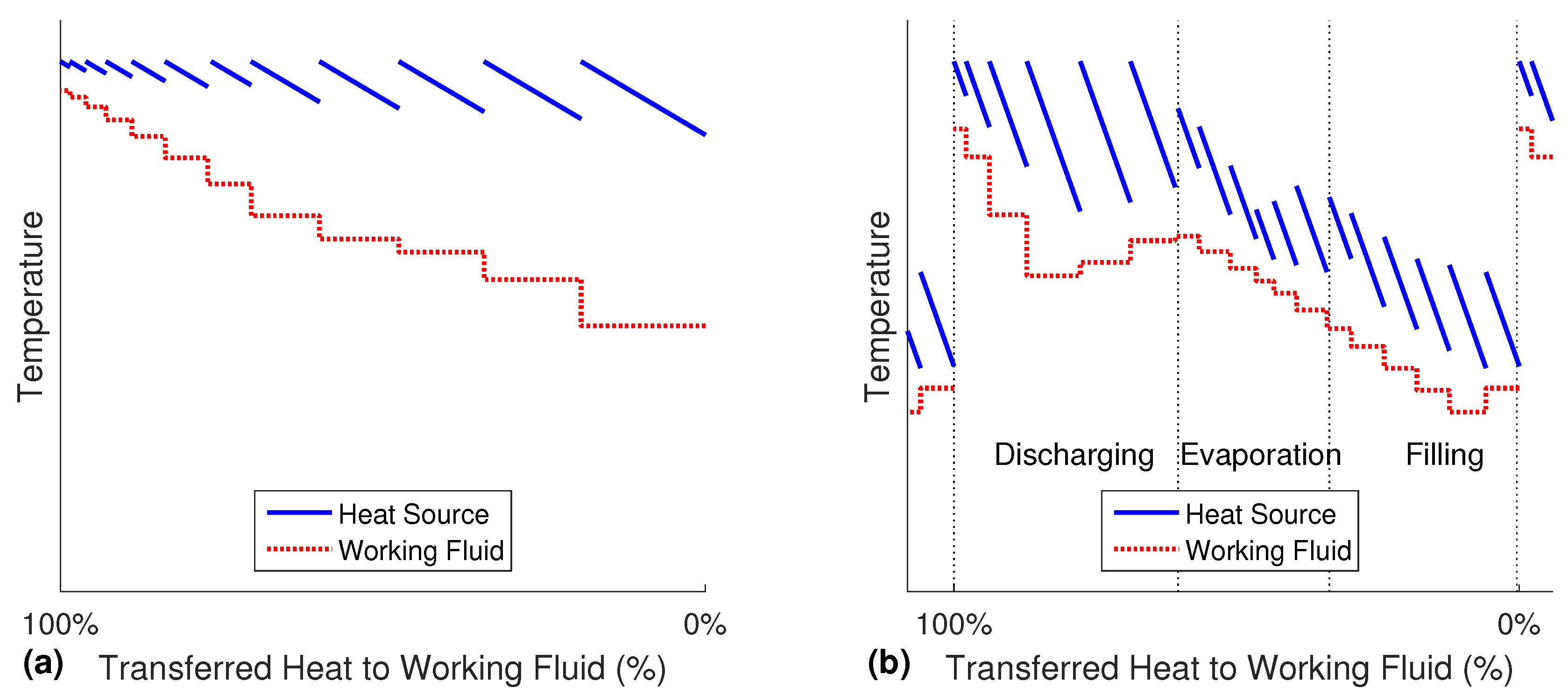
In the Misselhorn cycle, heat is transferred from one continuously flowing heat source to the pool of working fluid in the heat exchangers. The closed batch evaporation can best be explained in a piecewise Temperature-Heat-diagram (T-Q-diagram) of one heat exchanger, as presented in Figure 3a. For illustrative reasons, this figure of the evaporation sequence is divided into several theoretical displayed steps of the same duration (about 1 s). The actual calculations of the process are performed with a finer discretization between 0.05 s and 0.1 s (depending on the case).

Beginning with the lowest temperature of the working fluid on the right side, heat is transferred from the heat source medium to the working fluid. The pressure and the boiling temperature of the working fluid are assumed constant during one step, while the heat source is cooled down. In any following steps, the pressure and the corresponding boiling temperature of the working fluid are higher due to the isochoric process. As this is not a counter flow setup, but a sort of pool boiling, the working fluid is in exchange with fresh and hot heat source medium at all times. The rising temperature of the working fluid causes a decreasing temperature difference, and therefore, the transferred heat in each displayed step becomes smaller (the width of the steps decreases). Accordingly, the cooling of the heat source is reduced. As a result of the continuously rising boiling temperature, there is no distinct pinch point until the end of the evaporation.

It can be seen from Figure 3a that in the zone of hot working fluid, the outlet temperature of the heat source is still very high. Simultaneously, the cold part of the working fluid does not completely use the potential of the hot heat source. Therefore, the heat source flow is changed, so that it is not split, but rather flows through all heat exchanges in series. The fresh heat source medium is fed to the evaporator that is currently in the most important discharge phase (see Figure 3b). The outlet of every time step from this heat exchanger is then directed to the evaporation phase in the second heat exchanger and further to the third one. Although the outlet stream is gradually cooled down, its temperature is still high enough to preheat the inflowing cold working fluid. Once the operating phases are switched, the heat source flow has to be adjusted accordingly. The three cycle phases in Figure 3b can be seen as the simultaneous process in three different evaporators. The six steps in each of the phases are therefore happening at the same time as the corresponding steps in the other phases. As all of the heat exchangers are only shifted in time, but are similar apart from that, the whole red curve also matches a complete cycle in one single evaporator over time.

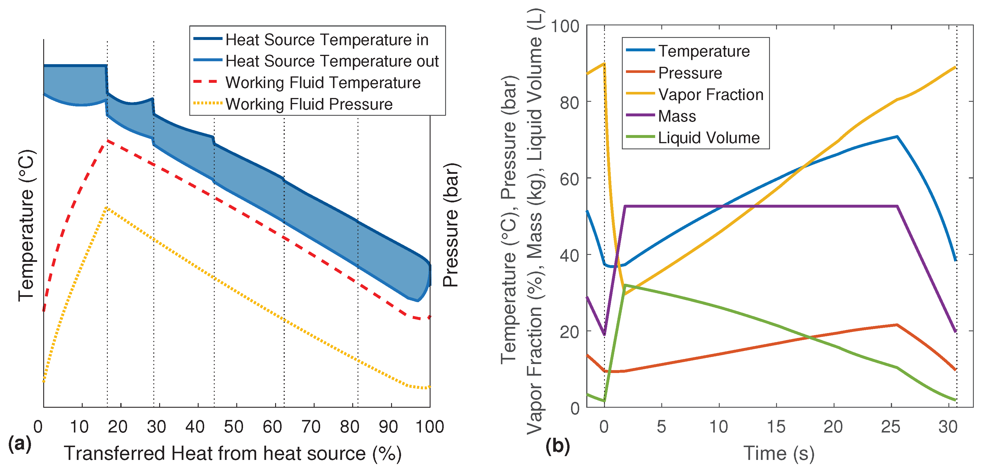
Since all three phases are heated, the pressure is already building up significantly in the filling phase. In order to preserve the advantage of the low power demand for the compression, the duration ratio of evaporation versus filling is adjusted. By adding three more evaporators, the cycle phases are now: filling, evaporation Phases 1 to 4 and discharge. In Figure 4a, the temperature profile of a setup with six heat exchangers is shown. By decreasing the size of the displayed steps, the graph flattens. For an infinitely small step size, the single lines of the cascading heat source would become vertical. Therefore, instead of many parallel lines, the inlet and outlet temperature of the heat source are displayed as two continuous graphs. The resulting T-Q-diagram shows the quasi-stationary and quasi-counter-flow process without any typical pinch point.

The six phases of the cycle are marked by the thin dotted lines. Like in Figure 3b, the one to the right is the filling, and the one to left is the discharging. It can be seen that the inlet temperature of the heat source is constant for the whole discharge phase, as explained earlier.

Figure 4b shows the variations of the system parameters over one complete evaporation cycle. While in the T-Q-diagrams, the filling phase is positioned on the right side, Figure 4b has to be read from left to right. Thus, the region left of 0 s is the end of the previous evaporation cycle. The temperature, pressure and vapor fraction rapidly decrease during the first few seconds due to the filling with cold working fluid. At the same time, the mass and the liquid volume of the working fluid increase. The temperature and pressure are then rising over the four evaporation phases. Although the evaporator is heated and there is still liquid in the evaporator during the following discharge phase, the re-evaporation cannot compensate the exhausting working fluid vapor. Therefore, the pressure is dropping, and the coupled boiling temperature results in a decreasing temperature of the working fluid. Only the vapor fraction further increases due to the re-evaporation of the remaining liquid.

3. Simulation Models

To evaluate the potential of the Misselhorn cycle, transient simulations are conducted in MATLAB^® R2016a (The MathWorks: Natick, MA, USA). For comparison, a common ORC is modeled in Aspen Plus^® V8.8 (Aspen Technology: Cambridge, MA, USA).

3.1. Aspen Model of the Benchmark ORC

The benchmark cycle is a common organic Rankine cycle without recuperator (see Figure 2b). The starting point for the simulations is the heat source with a fixed temperature and mass flow. The mass flow of the working fluid is adjusted to ensure the minimum pinch point in between the pre-heater and the evaporator. The sizes of the heat exchangers are adjusted automatically by the Aspen solver to fulfill the required heat transfer and to reach a superheating of 2 K for the live steam. The outlet pressure of the turbine is chosen to fit the available heat sink temperature with respect to the necessary pinch point in the condenser. Two auxiliary pumps are added to overcome the pressure drop of the heat source and heat sink in the pre-heater, the evaporator and the condenser. All pumps and the turbine are set up with constant isentropic efficiencies.

The outlet pressure of the feed pump is the only degree of freedom of the resulting model. It is varied in the context of a sensitivity analysis to find the best efficiencies.

3.2. MATLAB Model of the Misselhorn Cycle

Given the unsteady character of the Misselhorn cycle, a transient MATLAB model is developed. The cores of the model are the mass and energy balances of the evaporator shell side:

$$\frac{d{m}_{\text{WF,HX}}}{dt}={\dot{m}}_{\text{WF,in}}-{\dot{m}}_{\text{WF,out}}$$

(8)

$$\frac{d{U}_{\mathrm{HX}}}{dt}={\dot{H}}_{\text{WF,in}}-{\dot{H}}_{\text{WF,out}}+\dot{Q}$$

(9)

To solve the changes of the mass of the working fluid $m_{\mathrm{WF}}$ and of the internal energy $U_{\mathrm{HX}}$ in one evaporator, the mass flows (${\dot{m}}_{\text{WF,in}}$ and ${\dot{m}}_{\text{WF,out}}$), the enthalpy flows (${\dot{H}}_{\text{WF,in}}$ and ${\dot{H}}_{\text{WF,out}}$) and the heat flow $\dot{Q}$ that is transferred from the heat source are needed. All thermodynamic states are calculated with the REFPROP database V9.1 by NIST [16]. For this basic simulation, the heat exchangers are not modeled in detail. Instead, the initial heat transfer factor $k·A$ is assumed as constant and can be set in the context of parameter variations. During the evaporation, the overall factor $k·A$ is weighted by the current height of the liquid level. From the known inlet temperature of the heat source and the temperature of the working fluid, the transferred heat can be estimated using a stationary NTU approach [17] (Number of Transfer Units) for every discretized time step of the simulation. The nondimensional heat transfer ability

$$NTU=\frac{k·A}{{\dot{C}}_{\mathrm{HS}}}$$

(10)

can be calculated from the heat transfer coefficient k, the heat transfer area A and the heat capacity flow of the heat source ${\dot{C}}_{\mathrm{HS}}={\dot{m}}_{\mathrm{HS}}·c_{\text{p,HS}}$.

As the working fluid has a constant temperature over one time step, the heat exchanger efficiency ϵ is defined as

$$ϵ=1-exp(-NTU).$$

(11)

The actually transferred heat can then be obtained from the efficiency (Equation (11)) and the maximum possible heat transfer ${\dot{Q}}_{\max }$ by

$$\dot{Q}=ϵ·{\dot{Q}}_{\max }=ϵ·{\dot{C}}_{\mathrm{HS}}·\left(T_{\text{HS,in}}-T_{\text{WF,in}}\right)$$

(12)

Different heat transfer coefficients are estimated for the boiling liquid in the bottom part and the natural convection of the vapor phase in the upper part of the evaporator. The model also includes the changing liquid level during the evaporation. However, it does not consider the dwell time of the heat source medium in the evaporator, the heat capacity of the evaporator walls and the exact flow-dependent heat transfer coefficients. It is still well suited to gain insight into the general thermodynamic behavior of the Misselhorn cycle while being computationally efficient.

4. Results and Discussion

4.1. Reference Conditions

Both the simulations of the ORC and the Misselhorn cycle are based on the same reference case. The heat source and heat sink conditions are summarized in

Table 1. Reference case for heat source and heat sink.

Property	Heat Source (Water)	Heat Sink (Water)	Reference Conditions
Mass Flow	6.97 kg/s	Calculated from condenser pinch point	-
Temperature	85 °C	20 °C	20 °C
Pressure	3.1 bar	2.60 bar	1 bar

. Heat is available from hot water at the temperature of 85 °C with a fixed mass flow of 6.97 kg/s. Cold water at 20 °C is used in the condenser. The reference point for exergy calculations is set to 20 °C and 1 $\mathrm{bar}$. The total available exergy with these parameters is ${\mathit{Ex}}_{\mathrm{av}}$ = 184.6 kW.

The component and cycle parameters are summarized in

Table 2. Reference parameters of the cycle components.

Characteristic	Value	Characteristic	Value
Isentropic pump efficiency	90%	Working fluid	R134a
Isentropic turbine/engine efficiency	80 %	ORC pinch point	5 K
Pressure drop of heat source per HX	0.3 bar	Liquid to liquid heat transfer	1.5 kW/(m2 · K)
Pressure drop of working fluid per HX (ORC)	0.2 bar	Liquid to boiling heat transfer	3.0 kW/(m2 · K)

. As the main objective of the simulation of the Misselhorn cycle is the heat transfer, the power generation is simplified and calculated by the isentropic expansion of the produced vapor. To estimate the needed heat exchange area, the heat transfer coefficients are estimated as 1.5 kW/(m² · K) for liquid to liquid heat transfer, 3 kW/(m² · K) for liquid to boiling and 0.03 kW/(m² · K) for liquid to vapor. These values are obtained from the Aspen Exchanger Design and Rating tool for an exemplary plate heat exchanger suitable for this case. The given values are total heat transfer coefficients, which combine the heat transfer on both the hot and the cold side, as well as the wall resistance. As working fluid 1,1,1,2-Tetrafluoroethane (R134a) is used to be in agreement with the test system that is currently built by the Maschinenwerk Misselhorn MWM GmbH.

4.2. Performance of the Basic ORC

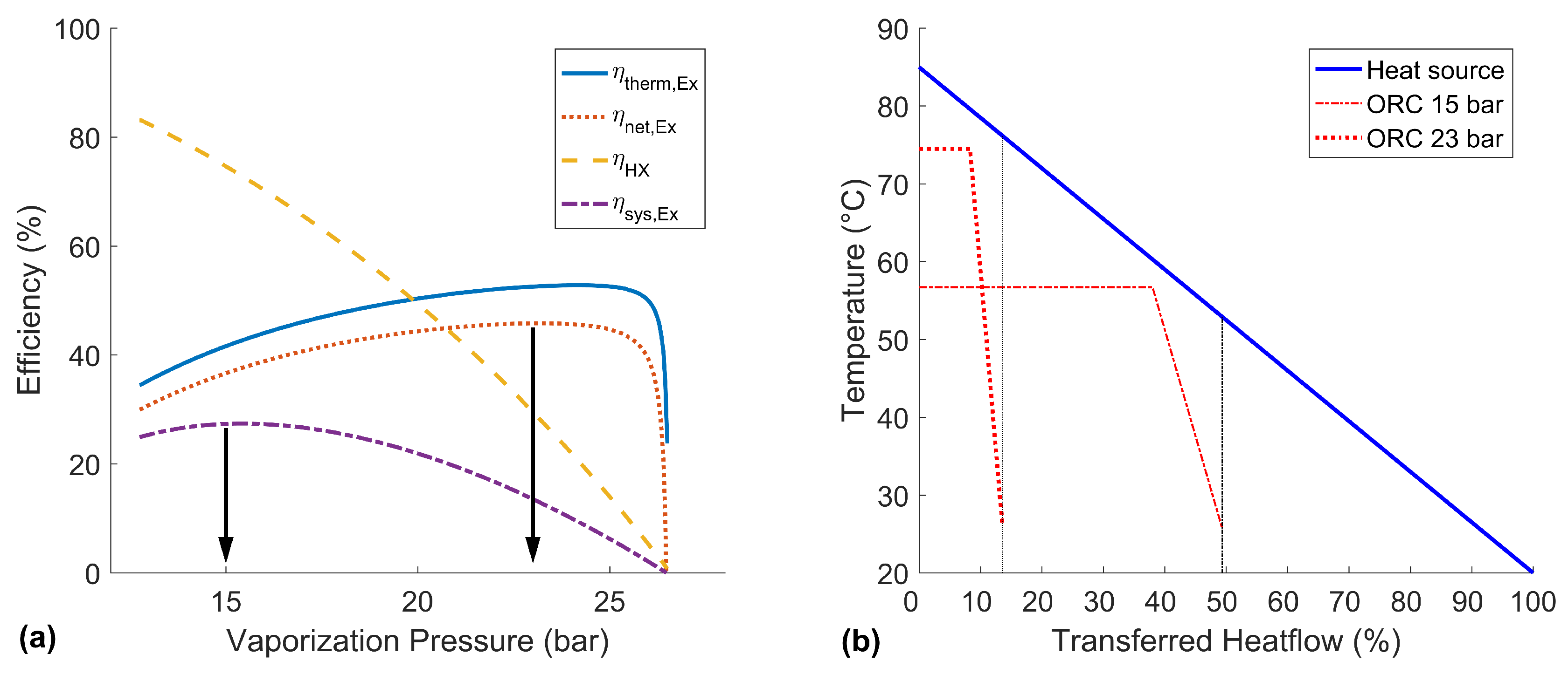
The optimization of the basic ORC can be conducted by a simple sensitivity analysis over the vaporization pressure. In Figure 5a, the influence of the vapor pressure on the ORC efficiencies is shown. It can be seen that the thermal/net exergy efficiencies and the heat exchanger efficiency are competing parameters. In terms of the target objective, the optimization of the exergetic system efficiency ${\eta }_{\text{sys,Ex}}$, this demands for a compromise of these values.

The best net exergy efficiency ${\eta }_{\text{net,Ex}}$ is reached at about 23 $\mathrm{bar}$. As the heat exchanger efficiency has no maximum in the investigated range, the best system efficiency at 15 $\mathrm{bar}$ is chosen as a second characteristic working point of this ORC. For further discussion, the T-Q-diagram of these two characteristic operating states is shown in Figure 5b.

The high pressure case shows a good temperature match with the heat source and reaches a high outlet temperature and pressure. As expected, a good net exergy efficiency of 45.7% can be gained. However, with the given pinch point, the heat exchanger efficiency is only 24.1%, and therefore, the gross power output (23.7 kW), as well as the system efficiency (11.0%) are low. A higher pressure would further increase the thermal exergy efficiency, but the transferred heat would become so small that the produced power could not even compensate the auxiliary power consumption.

In contrast, the lower pressure case can take advantage of the heat source much better, which is shown by a heat exchanger efficiency of 72.6%. The disadvantage is the comparably low net exergy efficiency of only 36.9%. Still, the exergetic system efficiency is at a global maximum of 26.8%, and the generated gross power of the turbine is at a maximum of 55.4 kW for this low pressure case. A lower pressure would allow an even better heat exchanger efficiency, but would not produce enough power in the turbine.

4.3. Performance of the Misselhorn Cycle

As a result of the transient character of the Misselhorn cycle, there are many degrees of freedom that affect the performance. Due to the extensive simulation duration, a simple parameter variation was not productive. Instead, a genetic algorithm is used to find the global maximum of the exergetic system efficiency ${\eta }_{\text{sys,Ex}}$.

The possible efficiency depends strongly on the number of used heat exchangers and their heat transfer ability. In addition to the setup with six heat exchangers (see Figure 4 on page 6), the basic setup with only three evaporators and an expanded setup with ten heat exchangers are shown in Figure 6a,b, respectively.

It can be seen that more heat exchangers allow a better temperature match and a higher maximum pressure. Consequently, the system efficiency can be raised from 29.8% with three heat exchangers up to 44.4% with ten heat exchangers. This improvement is based on an increasing net exergy efficiency (less exergy destruction), as well as a rising heat exchanger efficiency (less exergy losses). The displayed heat source temperature just right of the process is the average outlet temperature of the heat source that is leaving the process after the last phase.

4.4. Comparison of the Misselhorn Cycle and a Common Organic Rankine Cycle

The results of the Misselhorn cycle simulations in

Table 3. Results for the ORC and Misselhorn cycle.

Cycle Characteristics	ORC		MWM
	15 bar	23 bar	3 HX	6 HX	10 HX
$P_{\mathrm{output}}$	55.4 kW	23.7 kW	60.0 kW	78.0 kW	89.2 kW
$P_{\mathrm{pump}}$ (Feed/Auxiliary)	3.6/2.2 kW	2.0/1.3 kW	1.8/3.0 kW	1.4/4.4 kW	1.3/5.7 kW
$P_{\mathrm{net}}$	49.5 kW	20.4 kW	55.2 kW	72.3 kW	82.2 kW
${\dot{Q}}_{\mathrm{in}}$	944 kW	260 kW	968 kW	1230 kW	1367 kW
${\dot{\mathit{Ex}}}_{\mathrm{in}}$	134 kW	45 kW	136 kW	159 kW	168 kW
${\eta }_{\text{therm,Ex}}$	41.2%	53.1%	44.1%	49.2%	53.3%
${\eta }_{\text{net,Ex}}$	36.9%	45.7%	40.6%	45.6%	49.1%
${\eta }_{\text{HX,Ex}}$	72.6%	24.1%	73.5%	85.6%	90.5%
${\eta }_{\text{sys,Ex}}$	26.8%	11.0%	29.8%	39.0%	44.4%
Overall Area	29.6 m2	11.9 m2	37.0 m2	76.0 m2	126.4 m2
$T_{\text{HS,out}}$	52.7 °C	76.1 °C	52.1 °C	43.1 °C	38.4 °C

show a serious advantage over a common ORC. Already, the smallest setup with three heat exchangers shows an improvement of the system efficiency of more than 10% (ORC 26.8%/MWM 29.8%/+11.2%). Although they both transfer about the same amount of heat and exergy ($\dot{\mathit{Ex}}$ 135 kW, $\dot{Q}\approx$ 950 kW), the Misselhorn cycle offers better thermal and net efficiencies and therefore outperforms the ORC in the gross power output (55.4 kW/60.0 kW/+8.3%). In addition, the power needed of the feed pump is reduced.

Moreover, the single phase heat transfer in the pre-heater of the ORC requires a significant fraction of the overall heat transfer area of the low pressure ORC case. As the Misselhorn cycle takes only place in the two-phase region, the good heat transfer during boiling keeps the required transfer area of the additional heat exchangers at an acceptable value (29.6 m²/37.0 m²/+25%).

Simply increasing the exchanger area of the ORC and setting a smaller pinch point would allow for a small increase in the performance. However, there is no possibility to overcome the pinch point completely (see Figure 7).

In contrast, adding more heat exchangers to the Misselhorn cycle will significantly increase the performance. By using six evaporators, both the net exergy efficiency and the heat exchanger efficiency can be enhanced. Thus, the system efficiency can be improved by more than 40% compared to the ORC (26.8%/39.0%/+45.5%). The setup with ten heat exchangers can even top these numbers with a system efficiency of 44.4% (26.8%/44.4%/+65.7%). Of course, for this dimension, the required heat exchanger area is much bigger than for the ORC (30 m²/126 m²) (compare Figure 7).

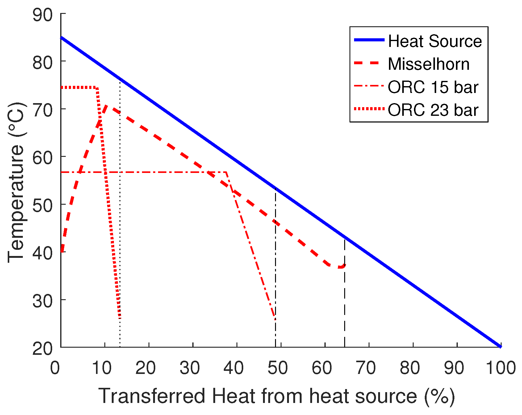
In general, the combination of a high maximum pressure of the working fluid with a good utilization of the heat source in the Misselhorn cycle allows for a clear thermodynamic advantage over a common ORC (see Figure 8).

5. Conclusions

The concept of the Misselhorn cycle was introduced with its two main characteristics: batch evaporation and a dynamic cascaded heat source circuit. This results in a good temperature match of the heat source and working fluid and allows for a good utilization of the available heat source at the same time.

Different efficiencies were defined in order to evaluate the performance of the Misselhorn cycle and to compare it to a common ORC. In this context, the exergy was used to illustrate the appearance of losses.

Based on a reference case, simulations of both a benchmark ORC and the Misselhorn cycle were performed. Depending on the number of used heat exchangers, the basic Misselhorn model showed an increase in the system efficiency (e.g., 10 evaporators, 44%) of up to 65% over the ORC (27%).

Deviations from this basic thermodynamic analysis should be analyzed in a detailed model of a plate heat exchanger, which includes the residence time of the heat source medium, the heat capacity and heat conduction of the heat exchanger material and detailed correlations for the heat transfer coefficients for pool boiling and convection. The model validation is planned based on measured data from a currently built test cycle. It is further planned to analyze the effects of different working fluids and to perform a thermo-economic evaluation.