Multi-Objective Optimization of Organic Rankine Cycle Power Plants Using Pure and Mixed Working Fluids ^†

Abstract

For zeotropic mixtures, the temperature varies during phase change, which is opposed to the isothermal phase change of pure fluids. The use of such mixtures as working fluids in organic Rankine cycle power plants enables a minimization of the mean temperature difference of the heat exchangers, which is beneficial for cycle performance. On the other hand, larger heat transfer surface areas are typically required for evaporation and condensation when zeotropic mixtures are used as working fluids. In order to assess the feasibility of using zeotropic mixtures, it is, therefore, important to consider the additional costs of the heat exchangers. In this study, we aim at evaluating the economic feasibility of zeotropic mixtures compared to pure fluids. We carry out a multi-objective optimization of the net power output and the component costs for organic Rankine cycle power plants using low-temperature heat at 90 ${}^{\circ }$C to produce electrical power at around 500 kW. The primary outcomes of the study are Pareto fronts, illustrating the power/cost relations for R32, R134a and R32/R134a (0.65/0.35${}_{\mathrm{mole}}$). The results indicate that R32/R134a is the best of these fluids, with 3.4 % higher net power than R32 at the same total cost of 1200 k$.

1. Introduction

The organic Rankine cycle (ORC) power plant is a technology that enables the utilization of low-temperature heat for electricity production. The working fluid selection for the ORC power plant is a critical design decision which affects the thermodynamic performance and the economic feasibility of the plant. The use of zeotropic mixtures as working fluids has been proposed as a way to improve the performance of the cycle [1]. Zeotropic mixtures change phase with varying temperature, which is opposed to the isothermal phase change of pure fluids. As the temperature of the heat source and heat sink change during heat exchange, zeotropic working fluids enable a closer match of the temperature profiles in the condenser and the boiler, compared to pure fluids. This results in a decrease in heat transfer irreversibilities and an increase in cycle performance. The condenser has been identified as the component where the irreversibilities are reduced the most due to matching of temperature profiles through optimization of mixture composition [2,3].

Heberle et al. [2] optimized the performance of ORC systems using zeotropic working fluids for utilization of geothermal heat at 120 ${}^{\circ }$C. Compared to pure isobutane, a mixture of isobutane/isopentane (0.9/0.1${}_{\mathrm{mole}}$) achieved an increase in the second law efficiency of 8%. They also compared the $UA$-values (the product of the overall heat transfer coefficient and the heat transfer area) of the heat exchangers in the cycle, and found that the mixture compositions resulting in the highest cycle performance also required the highest $UA$-values. This suggests that the cost of heat exchangers is larger when the mixture is used. Similar conclusions have been reached in studies where other mixtures and pure fluids have been compared based on thermodynamic performance (e.g., [4,5]). Previous literature, thereby, indicates that the feasibility of zeotropic mixtures should be evaluated by considering both thermodynamic and economic aspects.

Recent studies considered thermo-economic aspects in the performance evaluation of ORC systems [6,7,8,9,10,11,12,13,14,15]. Heberle and Brüggemann [6] carried out a thermodynamic optimization of zeotropic mixtures and pure fluids followed by an economic post-processing of the most promising mixtures and their pure fluids for heat source temperatures at 120 ${}^{\circ }$C and 160 ${}^{\circ }$C. The results indicated that the specific investment costs were higher for the mixtures. Nevertheless, the higher net power output enabled a lower electricity generation cost for the mixtures. For the 160 ${}^{\circ }$C case, propane/isobutane and R227ea/R245fa obtained a 4.0 % and 10.0 % reduction in the electricity generation cost compared to the best pure fluids in the mixtures. Le et al. [7] maximized the exergy efficiency and minimized the levelized cost of electricity for ORC systems using mixtures of R245fa and pentane as working fluids. Pure pentane was identified as the best fluid in both optimizations. In the minimization of the levelized cost of electricity, the minimum value for pentane was found to be 0.0863 $/kWh. The mixtures pentane/R245fa (0.05/0.95${}_{\mathrm{mass}}$) and pentane/R245fa (0.1/0.9${}_{\mathrm{mass}}$) obtained similar values at 0.0872 $/kWh and 0.0873 $/kWh, respectively. Feng et al. [8,9] carried out multi-objective optimizations of the levelized energy cost and the exergy efficiency for R245fa, pentane and R245fa/pentane mixtures. They selected the following cycle parameters as decision variables: evaporator outlet temperature, condenser temperature, degree of superheat and pinch point temperature difference. They focused the analyses on the variation of the levelized energy cost and the exergy efficiency as functions of the process parameters. Their results indicated that mixtures do not always show better thermodynamic and economic performance compared to pure fluids.

In the present study, we carry out a multi-objective optimization of net power output and component cost for an ORC power plant utilizing a low-temperature water stream at 90 ${}^{\circ }$C. To the knowledge of the authors, only a few recent studies [8,9,10,11] have considered a multi-objective optimization of thermodynamic and economic performance indicators for mixed working fluids. Compared to these previous studies, which included up to four cycle related decision variables, the present study includes a comprehensive selection of decision variables, i.e., five cycle parameters and six parameters defining the geometries of the heat exchangers. The objective of the study is to compare the performance of zeotropic mixtures to pure fluids based on equal values of equipment costs, thereby enabling a fair basis for comparison. The fluids considered are R32, R134a and R32/R134a (0.65/0.35${}_{\mathrm{mole}}$). These fluids are selected, since they achieved high thermodynamic performance at subcritical turbine inlet pressure in a previous study [5].

The paper begins with a description of the methodology in Section 2. The results are presented and discussed in Section 3 and conclusions are given in Section 4.

2. Methods

The multi-objective optimization method was developed in Matlab version 2014b [16] based on the framework described by Pierobon et al. [17]. The steady state ORC system model, capable of handling both pure fluids and mixtures through REFPROP^® version 9.1 [18], was adapted from a previous study [5] and integrated within the simulation tool. This model was previously validated by comparing results with similar models used by other authors [2,19,20,21]. 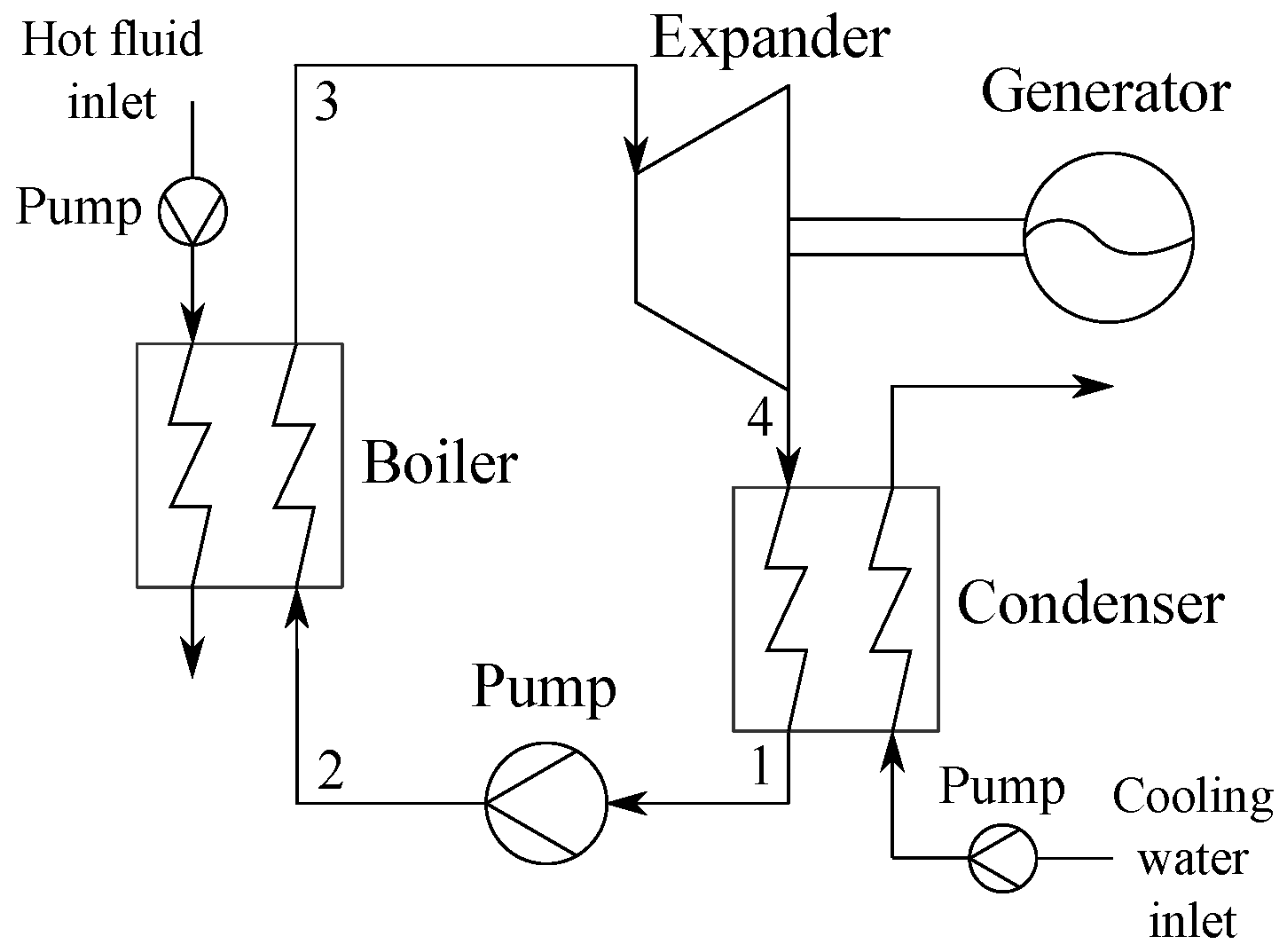The relative discrepancies were all below 3.3 % [5]. A sketch of the ORC power plant is depicted in Figure 1. 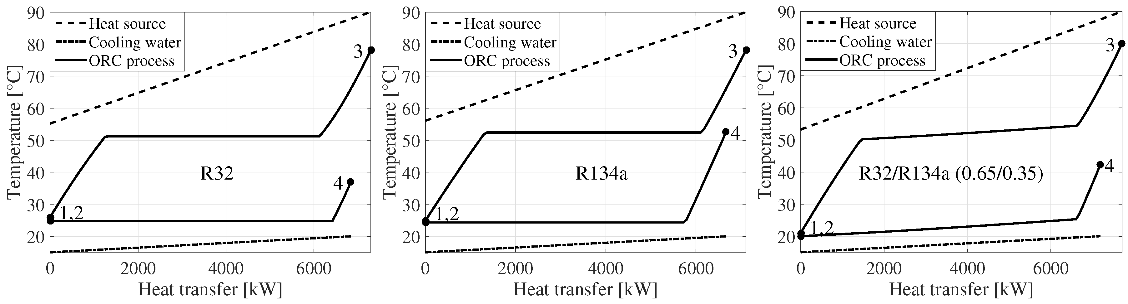Figure 2 displays $\dot{Q}$,T-diagrams of the maximum net power output solutions for R32, R134a and R32/R134a (0.65/0.35${}_{\mathrm{mole}}$) [5]. The composition of the mixture was the one which maximized the net power output of the cycle. At this composition, the temperature glide of condensation matched very well with the 5 ${}^{\circ }$C temperature increase of the cooling water, resulting in a minimization of the irreversibilities in the condenser; see Figure 2.

The selected heat source was a low-temperature water stream as was also investigated in Andreasen et al. [5].

Table 1. Modeling conditions.

Parameter Description	Value	Unit
Hot fluid (water)
Hot fluid inlet temperature	90	${}^{\circ }$C
Hot fluid mass flow	50	kg/s
Hot fluid pressure	4	bar
Condenser
Cooling water inlet temperature	15	${}^{\circ }$C
Cooling water pressure	4	bar
Working fluid pump
Isentropic efficiency	0.8	-
Auxiliary pumps
Isentropic efficiency	0.7	-
Turbine
Isentropic efficiency	0.8	-
Minimum outlet vapor quality	1	-

shows the hot fluid parameters along with the fixed input parameters assumed for the cycle. The hot fluid and cooling water pumps are denoted as auxiliary pumps.

The decision variables included cycle and heat exchanger design parameters—see

Table 2. Decision variables.

Parameter Description	Lower Bound	Upper Bound	Unit
Cycle parameters
Turbine inlet pressure	$P_{bub}(T_{cool,i}+30)$	$0.9·P_c$	bar
Superheating degree	0	40	${}^{\circ }$C
Condensing temperature at bubble point	$T_{cool,i}+5$	$T_{cool,i}+20$	${}^{\circ }$C
Boiler pinch point temperature	0.1	20	${}^{\circ }$C
Condenser pinch point temperature	0.1	20	${}^{\circ }$C
Condenser design
Inner tube diameter	16	26	mm
Number of tubes	10	200	-
Baffle spacing	$0.5·d_s$	$3·d_s$	mm
Boiler design
Inner tube diameter	16	26	mm
Number of tubes	10	200	-
Baffle spacing	$0.5·d_s$	$3·d_s$	mm

. The lower boundary for the turbine inlet pressure was defined as the bubble point pressure at a temperature 30 ${}^{\circ }$C higher than the cooling water inlet temperature ($T_{cool,i}$), and the upper boundary was 90% of the critical pressure ($P_c$). The superheating degree was defined as the temperature difference between the dew point temperature and the turbine inlet temperature, and the bounds for the baffle spacing were set relative to the shell diameter ($d_s$). The lower bounds for the pinch points in the condenser and the boiler were set to 0.1 ${}^{\circ }$C. Such low pinch points are not feasible in practice, but they were allowed in this study in order to compare the fluids based on a wide range of equipment costs.

The objective functions for the optimization were the net power output and the total cost of the components. The net power was calculated as:

$${\dot{W}}_{NET}={\dot{m}}_{wf}(h_3-h_4-(h_2-h_1))-{\dot{W}}_{aux.,pumps}$$

(1)

where ${\dot{m}}_{wf}$ was the working fluid mass flow, h was the mass specific enthalpy and ${\dot{W}}_{aux.,pumps}$ was the power consumption of the hot fluid and cooling water pumps. The total cost ($C_{tot}$) of the components was found by adding the cost of the turbine ($C_{turb}$), working fluid pump ($C_{wf,pump}$), condenser ($C_{cond}$), boiler ($C_{boil}$), generator ($C_{gen}$) and the two auxiliary pumps ($C_{aux.,pumps}$):

$$C_{tot}=C_{turb}+C_{wf,pump}+C_{cond}+C_{boil}+C_{gen}+C_{aux.,pumps}$$

(2)

The total cost considered in this paper was the equipment cost, thus further expenses can be expected for the construction of the ORC power plants, e.g., installation costs.

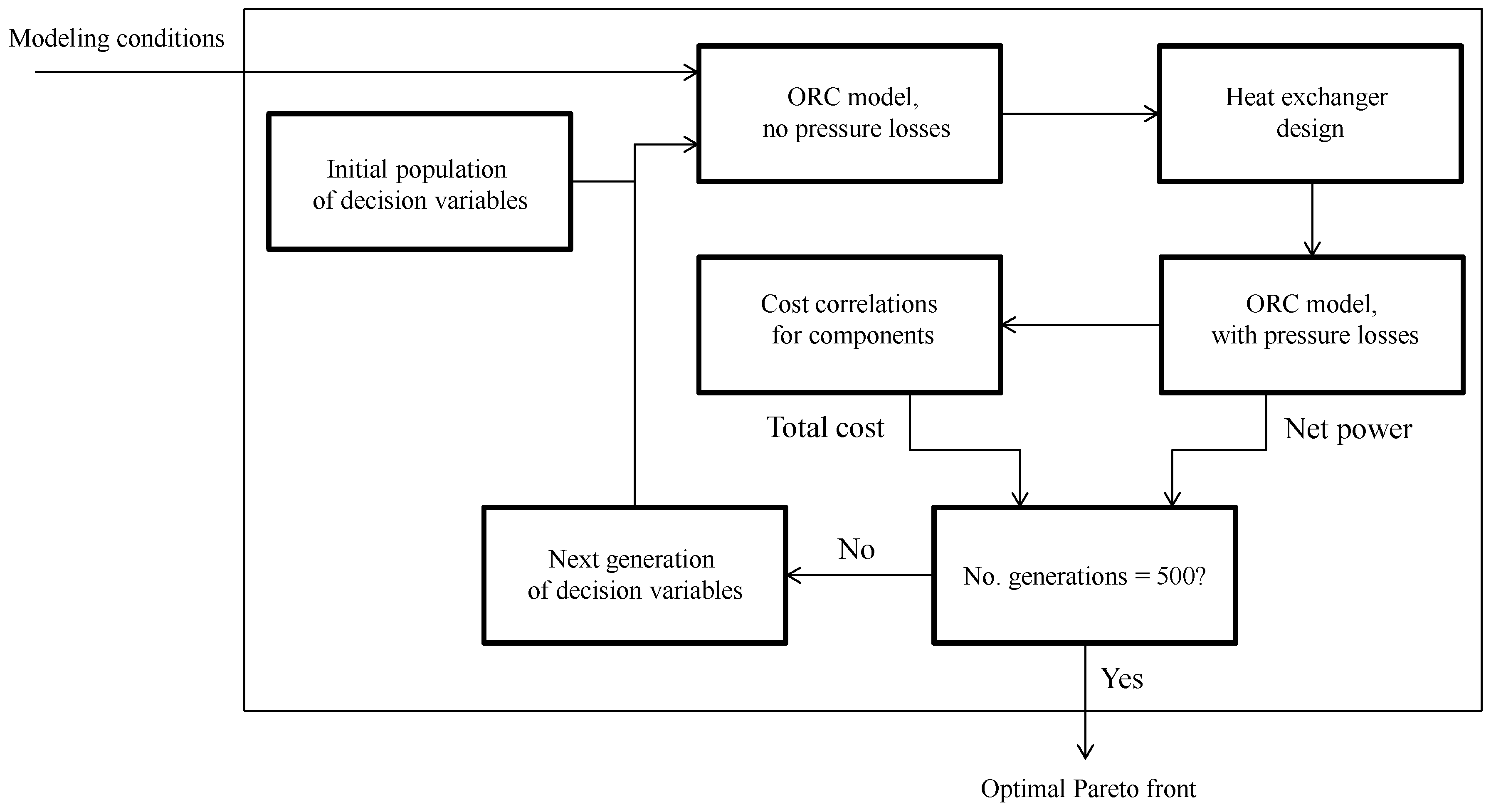
The optimization framework is sketched in Figure 3 and comprised the following steps [17]:

• Calculation of the process states by use of the cycle model (without pressure losses)
• Layout of the geometry of the condenser and the boiler and calculation of the heat transfer area and the pressure losses
• Calculation of the net power output by use of the cycle model (with pressure losses)
• Calculation of the total component cost

The optimizer was the genetic algorithm optimizer integrated in Matlab version 2014b [16]. The number of generations was 500 and the population size was 30,000.

2.1. Heat Exchanger Modeling

The heat exchanger models were developed based on the shell-and-tube model used in Kærn et al. [22]. In order to avoid leakage of working fluid, which for zeotropic mixtures can result in undesirable composition shifts, both the boiler and the condenser were designed with the working fluid flowing inside the tubes [23]. The heat exchangers were designed as TEMA (Tubular Exchanger Manufacturers Association) E type shell-and-tube heat exchangers with one shell pass and one tube pass. A 60${}^{\circ }$ triangular tube layout was used—see Figure 4.

Table 3. Heat exchanger modeling conditions.

Parameter Description	Value/Range	Unit
Tube configuration	Triangular tube 60${}^{\circ }$	-
Tube thickness	3	mm
Tube pitch	$1.5·d_{ou}$	mm
Baffle cut	$0.25·d_s$	mm
Tube wall conductivity	16	W/mK
Number of control volumes	30	-
Condenser velocities
Tube side inlet	$5-22$	m/s
Tube side outlet	$0.5-4$	m/s
Shell side inlet	$0.3-1.5$	m/s
Boiler velocities
Tube side inlet	$0.9-4$	m/s
Tube side outlet	$5-22$	m/s
Shell side inlet	$0.3-1.5$	m/s

lists the modeling conditions used for the shell-and-tube heat exchangers including the geometric parameters and the ranges for the flow velocities. The velocities must be high enough to avoid excessive fouling, but not so high that the heat exchanger material is eroded. The boundaries for the flow velocities were selected based on recommendations from Nag [24], Shah and Sekulić [25] and Coulson et al. [26]. The shell side velocity was only checked at the inlet, since the density variations of the hot fluid and the cooling water were small. The tube side outlet velocity for the condenser was allowed to be lower than the minimum value of 0.9 m/s for liquid in-tube flow found in Shah and Sekulić [25]. Full liquid flow was only present at the end of the condenser tube as all vapor was condensed. It was, therefore, assumed that the liquid velocity could reach 0.5 m/s at the condenser outlet without the risk of excessive fouling formation.

The heat transfer and pressure drop characteristics on the shell side were estimated based on the Bell–Delaware method [25]. The method was implemented for tubes without fins and for a shell design without tubes in the window section. The effects of larger baffle spacings at the inlet and outlet ducts compared to the central baffle spacing were neglected.

For single-phase flow, the heat transfer coefficient was calculated using the correlation provided by Gnielinski [27]. The two-phase heat transfer coefficient of boiling was estimated based on the correlation provided by Gungor and Winterton [28] and Thome [29]:

$${\alpha }_{2p,boil}={\alpha }_L\left[1+3000{\left(Bo{F}_c\right)}^{0.86}+1.12{\left(\frac{x}{1-x}\right)}^{0.75},{\left(\frac{{\rho }_L}{{\rho }_V}\right)}^{0.41}\right]$$

(3)

where $Bo$ was the boiling number, x was the vapor quality, ${\rho }_L$ was the density of saturated liquid, ${\rho }_V$ was the density of saturated vapor and ${\alpha }_L$ was the liquid heat transfer coefficient which was calculated using the Dittus–Boelter correlation [30]. The ratio of the nucleate boiling heat transfer coefficient to the ideal nucleate boiling heat transfer coefficient, $F_c={\alpha }_{nb}/{\alpha }_{nb,id}$, was calculated by

$$F_c={\left[1+\left(\frac{{\alpha }_{nb,id}}{q_{nb}}\right)(T_{dew}-T_{bub})\left[1-exp\left(\frac{-B{q}_{nb}}{{\rho }_L{h}_{LV}{\beta }_L}\right)\right]\right]}^{-1}$$

(4)

where $q_{nb}$ was the nucleate boiling heat flux, $T_{dew}$ was the dew point temperature, $T_{bub}$ was the bubble point temperature, B was a scaling factor, $h_{LV}$ was the enthalpy of vaporization, and ${\beta }_L$ was the liquid phase mass transfer coefficient. The values of B and ${\beta }_L$ were set to $B=1$ and ${\beta }_L=0.0003$ m/s according to Thome [29]. The ideal nucleate boiling heat transfer coefficient, ${\alpha }_{nb,id}$ was calculated using the correlation by Stephan and Abdelsalam [31].

For in-tube condensation, the heat transfer coefficient was estimated using the following correlation by Shah [32]:

$${\alpha }_{2p,cond}=\left\{\begin{array}{cc}{\alpha }_I,\hfill & J_g\ge 0.98{(Z+0.263)}^{-0.62}\hfill \\ {\alpha }_I+{\alpha }_{Nu},\hfill & J_g<0.98{(Z+0.263)}^{-0.62}\hfill \end{array}\right.$$

(5)

where Z was Shah’s correlating parameter and $J_g$ was the dimensionless vapor velocity. These two parameters were calculated as:

$$Z={P_r}^{0.4}{\left(\frac{1}{x}-1\right)}^{0.8}$$

(6)

$$J_g=\frac{xG}{{\left(g{d}_{in}{\rho }_V({\rho }_L-{\rho }_V)\right)}^{0.5}}$$

(7)

where $P_r$ was the reduced pressure, and g was the gravitational acceleration.

The heat transfer coefficients ${\alpha }_I$ and ${\alpha }_{Nu}$ were calculated as:

$${\alpha }_I={\alpha }_{LT}{\left(\frac{{\mu }_L}{14{\mu }_V}\right)}^{0.0058+0.557P_r}\left[{(1-x)}^{0.8}+\frac{3.8x^{0.76}{(1-x)}^{0.04}}{{P_r}^{0.38}}\right]$$

(8)

$${\alpha }_{Nu}=1.32{R{e}_L}^{-1/3}{\left[\frac{{\rho }_L({\rho }_L-{\rho }_V)g{{\lambda }_L}^3}{{{\mu }_L}^2}\right]}^{1/3}$$

(9)

where ${\alpha }_{LT}$ was the heat transfer coefficient assuming all mass to be flowing as liquid and $R{e}_L$ was the Reynolds number for the liquid phase only. The variable ${\alpha }_{LT}$ was calculated using the Dittus–Boelter equation [30]. For mixtures the heat transfer coefficient obtained from equation (5) was corrected using the method proposed by Bell and Ghaly [33]. For in-tube flow, the single-phase pressure drops were calculated based on the Blasius equation [34] and the two-phase pressure drops were calculated using the correlation by Müller-Steinhagen and Heck [35].

The heat exchangers were discretized in 30 control volumes defined by equal enthalpy differences. The local properties, and consequently the heat transfer coefficient, pressure drop and required heat transfer area, were calculated for each control volume. The heat transfer area and pressure drop were subsequently added for all control volumes to give the total area and pressure drops for the heat exchangers.

The heat exchanger models were based on the heat recovery boiler model presented by Kærn et al. [22], which was verified by comparing the results to the results obtained by Stecco and Desideri [36]. The total heat transfer area was predicted within 6%. The implementation of the Bell–Delaware method was verified using examples 8.3 and 9.4 outlined by Shah and Sekulić [25]. The implementation of the Bell–Delaware method matched with the results outlined in the two examples to rounding accuracy with discrepancies below 0.15%. The implementations of the two-phase heat transfer correlations in Equations (3) and (5) were verified by comparing the results to the results presented for the mixture R404A (R125/R143a/R134a (0.44/0.52/0.04${}_{\mathrm{mass}}$)) by Thome [29] (in Figure 14c) and Shah [32] (in Figure 6). The implementations of the equations were verified for vapor qualities at 0.2, 0.4, 0.6 and 0.8, and showed discrepancies below 1.1% for Equation (3) and below 2.5% for Equation (5). The discrepancies were mainly due to inaccuracies in obtaining the reference data from the figures, thus other deviations are expected to be negligibly small.

2.2. Cost Correlations

The cost (in US$) of the components in the cycle were estimated based on correlations found in the literature. The turbine was assumed to be axial, since axial turbines are commonly used by manufacturers in the range of power (approximately 50–600 kW) considered in the present paper [37]. The cost (in €) of the turbine was estimated based on the correlation provided by Astolfi et al. [38]:

$$C_{turb}=1.230·{10}^6{\left(\frac{1}{2}\right)}^{0.5}{\left(\frac{\sqrt{{\dot{V}}_4}/{(\Delta h_{is})}^{0.25}}{0.18}\right)}^{1.1}$$

(10)

where ${\dot{V}}_4$ was the volume flow at the turbine outlet and $\Delta h_{is}$ was the isentropic enthalpy drop across the turbine. A euro-to-dollar conversion factor of 1.2 was used to convert the turbine cost to US$.

The costs of the pumps, the heat exchangers and the generator were estimated by:

$$C_E=C_B{\left(\frac{Q}{Q_B}\right)}^M{f}_M{f}_P{f}_T$$

(11)

where $C_E$ was the equipment cost for equipment with capacity Q, $C_B$ was the base cost for equipment with capacity $Q_B$, M was a constant exponent, and $f_M$, $f_P$ and $f_T$ were correction factors accounting for materials of construction, design pressure and design temperature.

The economic parameters needed in the cost correlation are listed in

Table 4. Economic parameters.

Component	$C_B$	$Q_B$	M	$f_M$	$f_P$	$f_T$	Reference
Heat exchangers	32.8 k$	80 m${}^2$	0.68	1.7	[39]	1	[39]
Pumps	9.48 k$	4 kW	0.55	1	1	1	[39]
Generator	3.7 k$	1000 kW	0.95	1	1	1	[40]

. For the heat exchangers, the pressure correction factor was obtained by linear interpolation between the values reported in Smith [39]. The component costs were converted to 2014 values by using the Chemical Engineering Plant Cost Index.

3. Results and Discussion

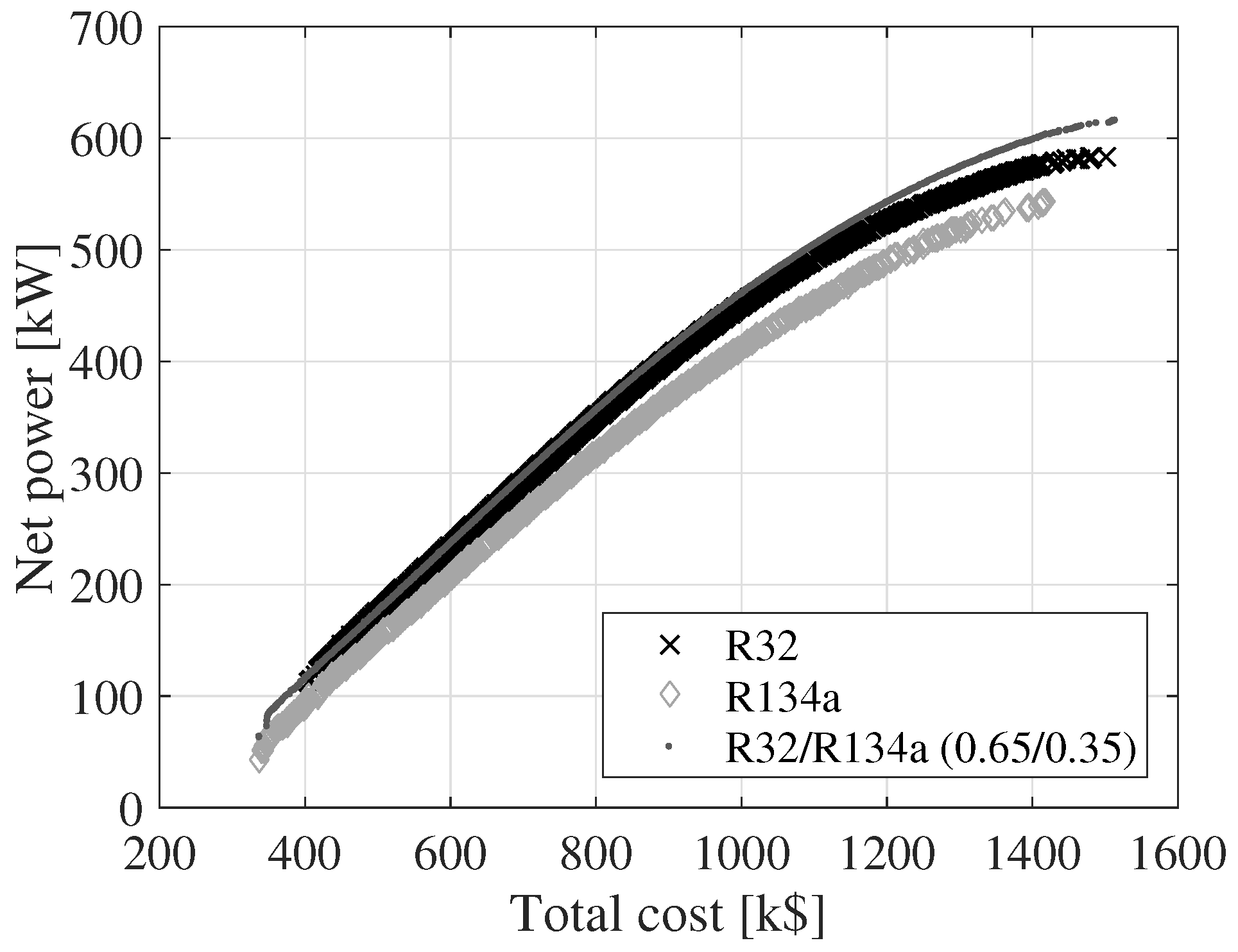
Figure 5 shows the Pareto fronts for multi-objective optimizations of net power output and cost for R32, R134a and R32/R134a (0.65/0.35). The results indicate that R32/R134a is the best of the three fluids, since it enables the highest net power output at the lowest component cost. R32 is the second best fluid while R134a is performing worst.

When the fluids are compared based on a single-objective optimization of net power output, R32/R134a (0.65/0.35) reaches 13.8% higher net power output than R32 and 14.6% higher than R134a [5]. However, this approach does not account for the equipment cost, and it was therefore not ensured that the fluids were compared based on similar cost. The multi-objective optimization, on the other hand, does enable a fluid comparison based on fixed equipment cost. For a total cost of 1200 k$, R32/R134a reaches a 3.4% higher net power than R32 and 10.9% higher than R134a. At $C_{tot}=800$ k$, the mixture obtains 2.1% higher net power than R32 and 12.6% higher than R134a. It should be noted that in the single-objective optimization, which was presented in Andreasen et al. [5], the mixture composition was optimized, but, in the multi-objective optimization carried out in the present paper, it is not. It is, therefore, possible that higher performance can be achieved with the mixture if the composition is optimized in the multi-objective optimization.

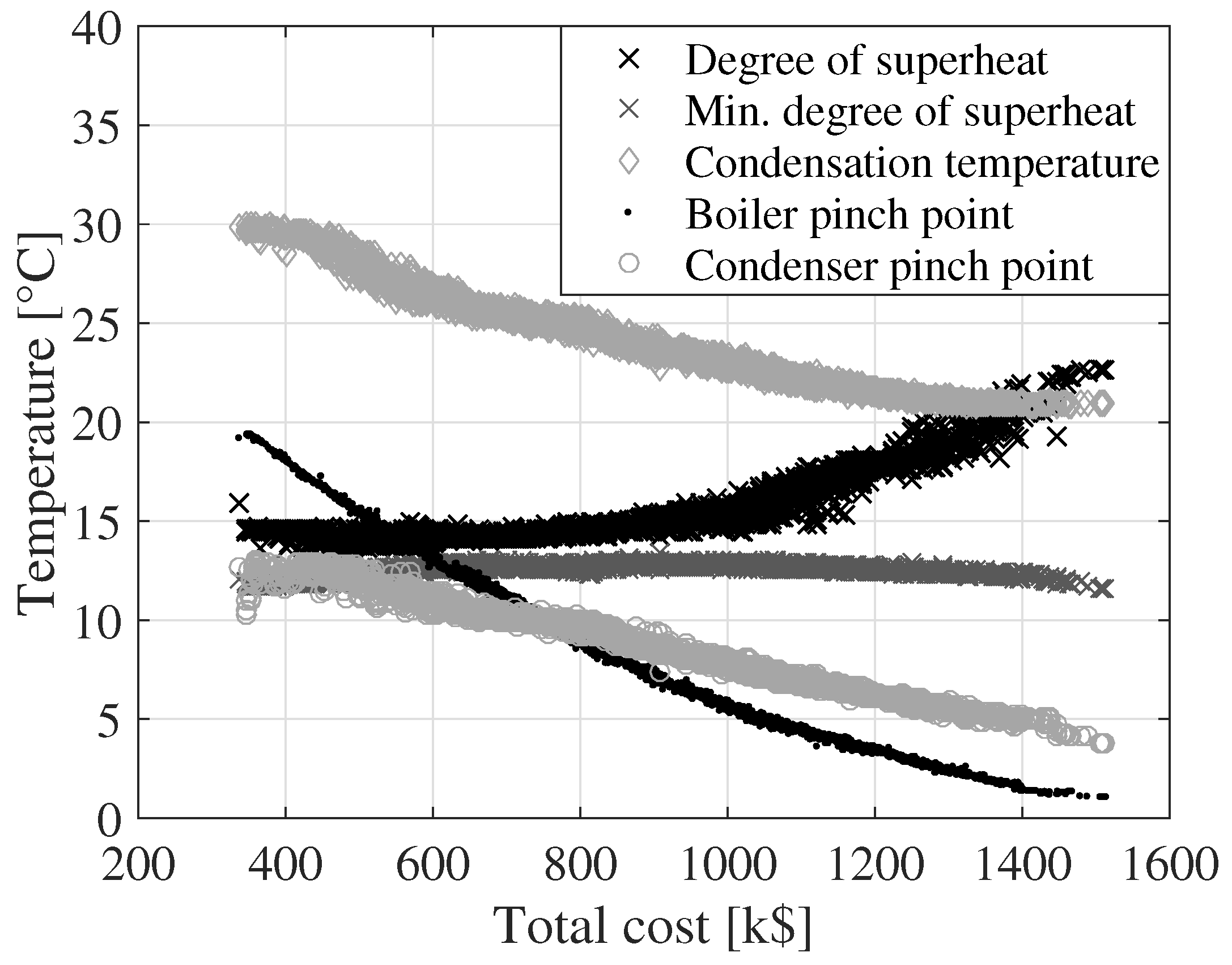
In Figure 6, the optimal degree of superheating, the minimum degree of superheating ensuring dry expansion, the condensing temperature (defined at the bubble point), the boiler pinch point and the condenser pinch point are plotted as a function of the total cost for R32/R134a. The degree of superheating increases from about 13 to 23 ${}^{\circ }$C as the total component cost increases. The minimum degree of superheat is calculated as the degree of superheat which results in saturated vapor condition at the outlet of the turbine. This minimum limit on the degree of superheat varies from 11 to 14 ${}^{\circ }$C due to variations in the condensing and boiling pressures. The results from the previous single objective maximization of net power output for R32/R134a indicated that a degree of superheat around 26 ${}^{\circ }$C resulted in optimal performance [5]. The results presented in Figure 6 indicate that the degree of superheat should be close to the minimum possible value at $C_{tot}<1000$ k$. At $C_{tot}>1000$ k$, superheating becomes increasingly beneficial as the total cost increases. Since the heat transfer coefficient for vapor flow is lower than those of liquid and two-phase flow, the heat transfer in the superheater section requires more heat transfer area compared to the evaporator and preheater sections. Thereby, when the total component cost is low, the results suggest that it is feasible to have a low degree of superheat and focus the available investment, or heat transfer area, on decreasing the pinch point in the boiler and the condensation pressure. At around $C_{tot}>1000$ k$, it becomes feasible to allocate heat transfer area to the superheater and thereby increase the degree of superheat which, for R32/R134a (0.65/0.35), is thermodynamically beneficial.

The condensing temperature, boiler pinch point and condenser pinch point all continuously decrease as the total component cost increases. The decrease in boiler pinch point results in an increase in the heat input to the cycle. This trend positively affects the net power output while increasing the investment cost for the boiler. The decrease in the condensing temperature has a positive effect on net power output, but requires larger heat transfer areas since the temperature difference between the cooling water and the condensing working fluid decreases. The larger heat transfer areas result in higher investment costs for the condenser. For fixed cycle conditions (condensing temperature, mass flow, etc.), the condenser pinch point only affects the net power output of the cycle through the power consumption of the cooling water pump. The pinch point temperature of the condenser thereby primarily affects the cost of the condenser. Therefore, the condenser pinch point tends to be as large as possible, while respecting the following constraints: (1) the cooling water outlet temperature must be larger than the inlet temperature and (2) the flow velocity in the condenser shell should not be higher than 1.5 m/s. A high condenser pinch point results in a low cooling water temperature increase and thereby a high cooling water mass flow and a high shell flow velocity. For R32/R134a, the temperature glide of condensation is varying from 5.0 ${}^{\circ }$C to 5.3 ${}^{\circ }$C, while the cooling water temperature increase ranges from 5.7 to 14.5 ${}^{\circ }$C. In thermodynamic analyses of zeotropic mixtures, optimum conditions are typically obtained when the temperature glide of the mixture and the temperature increase of the cooling water are matched [2,3,5,19]. However, the present study indicates that, when considering both performance and cost, it is beneficial that the temperature increase of the cooling water is larger than the temperature glide of condensation.

For total costs of 1300 k$, the boiler pinch point drops below 2.5 ${}^{\circ }$C. It is unusual that solutions with pinch points below 2.5 ${}^{\circ }$C represent economically feasible solutions. In Figure 5 at a total cost of 1300 k$, the curves are leveling off, meaning that an increase in investment cost results in a low increase in net power output compared to when the total cost is lower. It is therefore likely that the more economically feasible solutions are found at total costs below 1300 k$. It should be noted that the Pareto fronts do not provide information which directly can be used to make an investment decision, since they do not include information about the possible income related to the power delivered by the ORC power plant. Such information is necessary in order to estimate, e.g., net present value or payback periods, which are useful figures for making investment decisions. The Pareto fronts should rather be used for assessing the feasibility of working fluids based on equal component costs, thereby ensuring a fair basis for comparison.

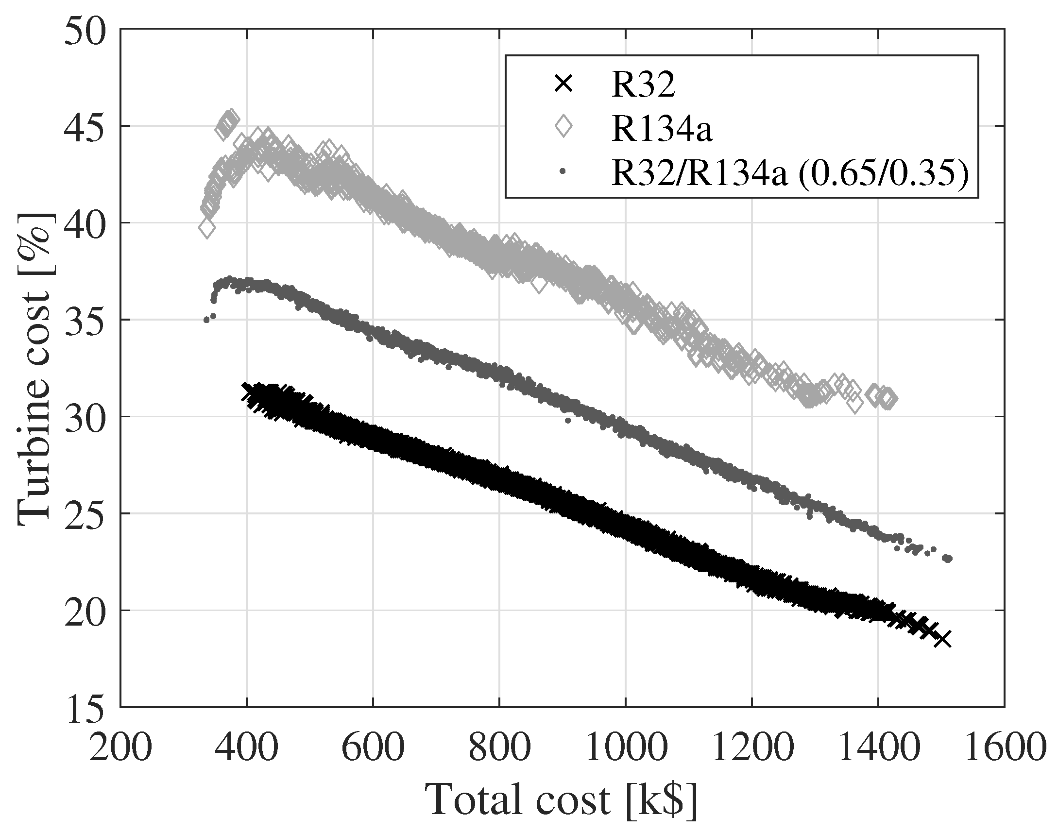
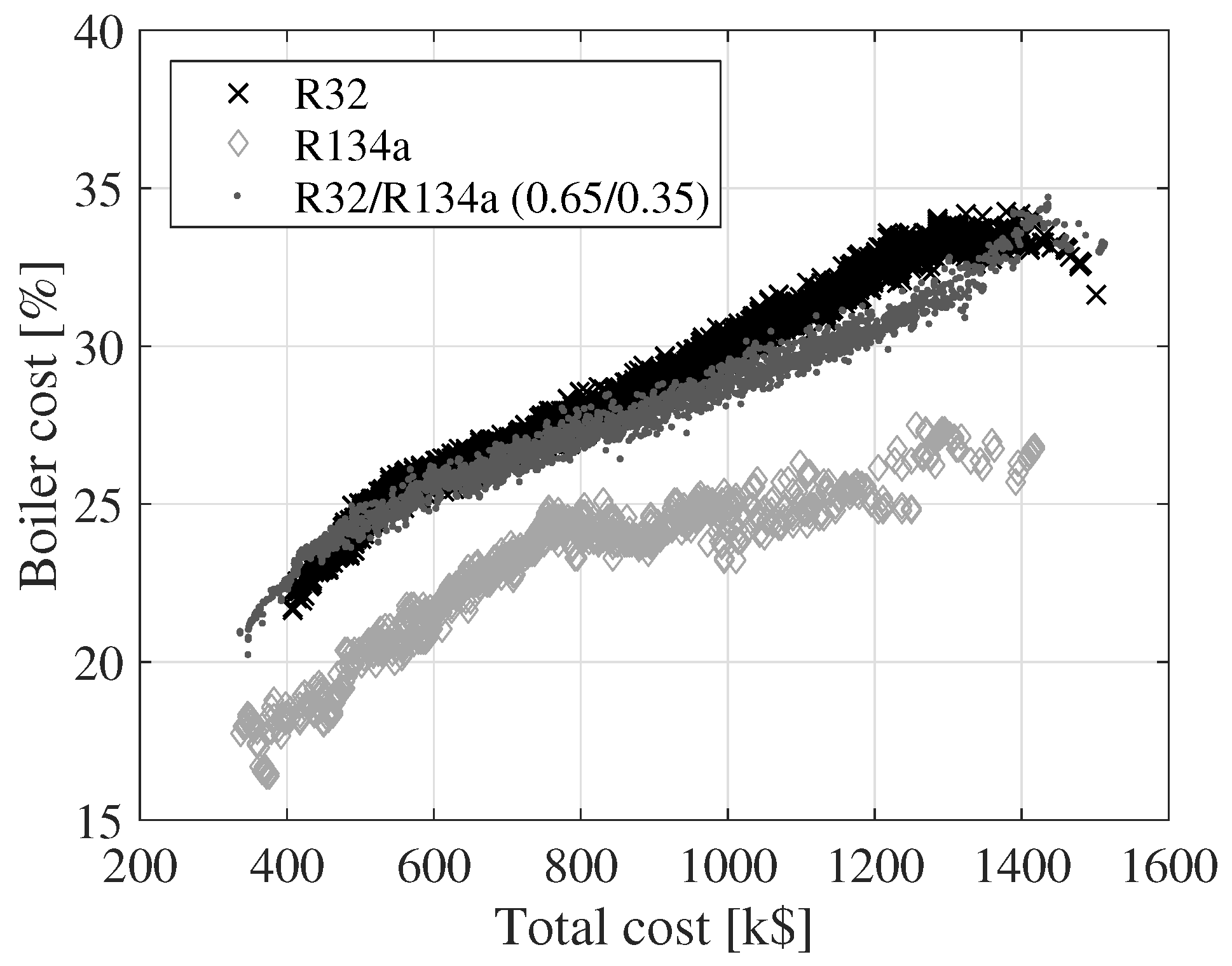
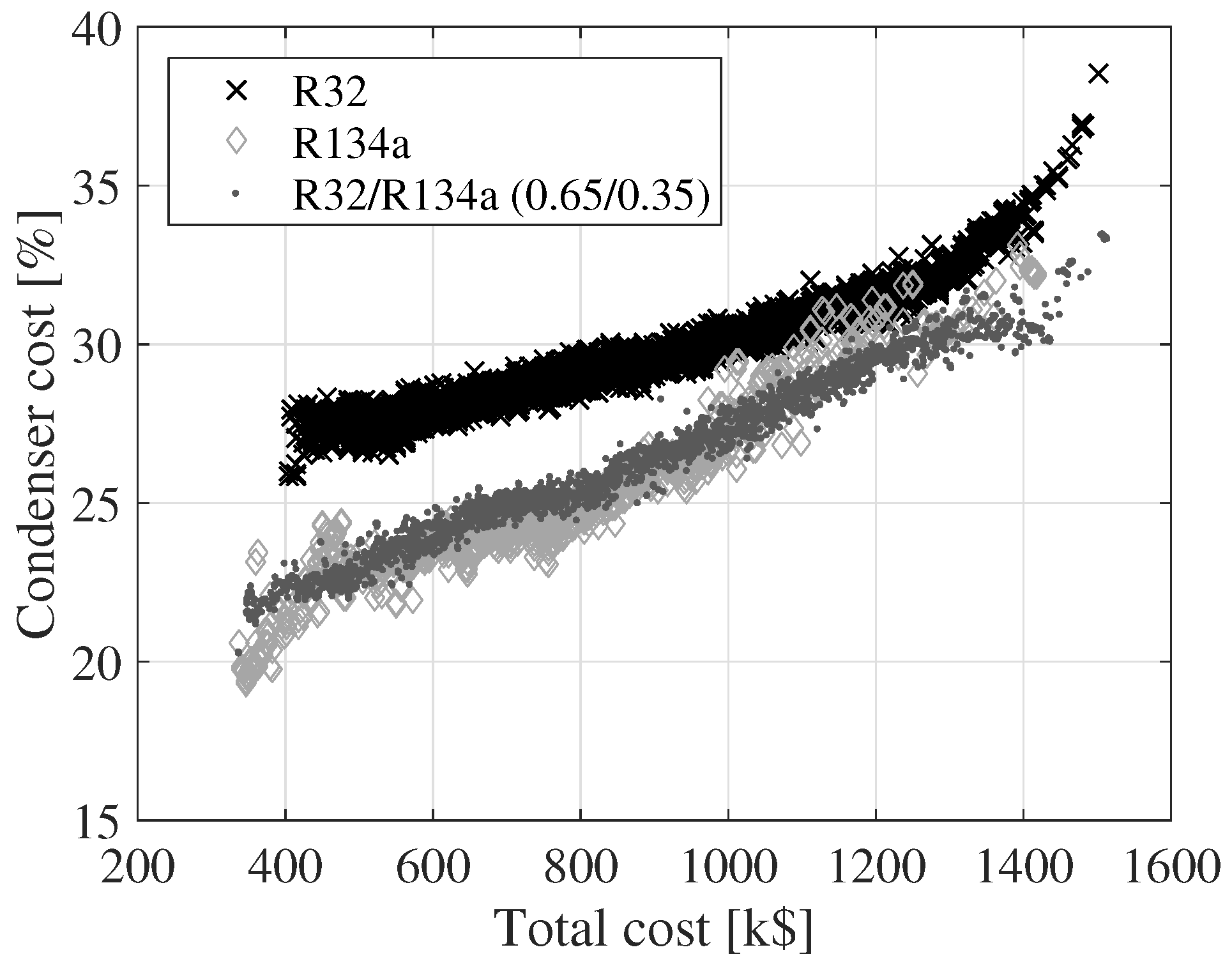
Figure 7, Figure 8 and Figure 9 show the variation of the cost of the turbine, condenser and boiler as a function of the total cost for the three fluids. The cost values displayed on the y-axes are relative to the total cost. The relative size of the turbine cost decreases, while the relative costs of the condenser and boiler increase. The relative turbine costs decrease since the turbine cost is a function of the outlet volume flow rate and the isentropic enthalpy drop. An increase in the outlet volume flow rate or a decrease in the isentropic enthalpy drop results in an increase in the turbine cost. These two parameters can be varied by changing, e.g., the boiler pressure or the turbine inlet temperature. By modifying the boiler pressure or the turbine inlet temperature, it is, however, not guaranteed that the net power output increases. The cost of the condenser and the boiler can be increased by decreasing the pinch point temperatures of the heat exchangers or the condensing temperature. This has a positive effect on the net power output. Thus, the costs of the heat exchangers are not as tightly connected to the cycle parameters as the turbine is.

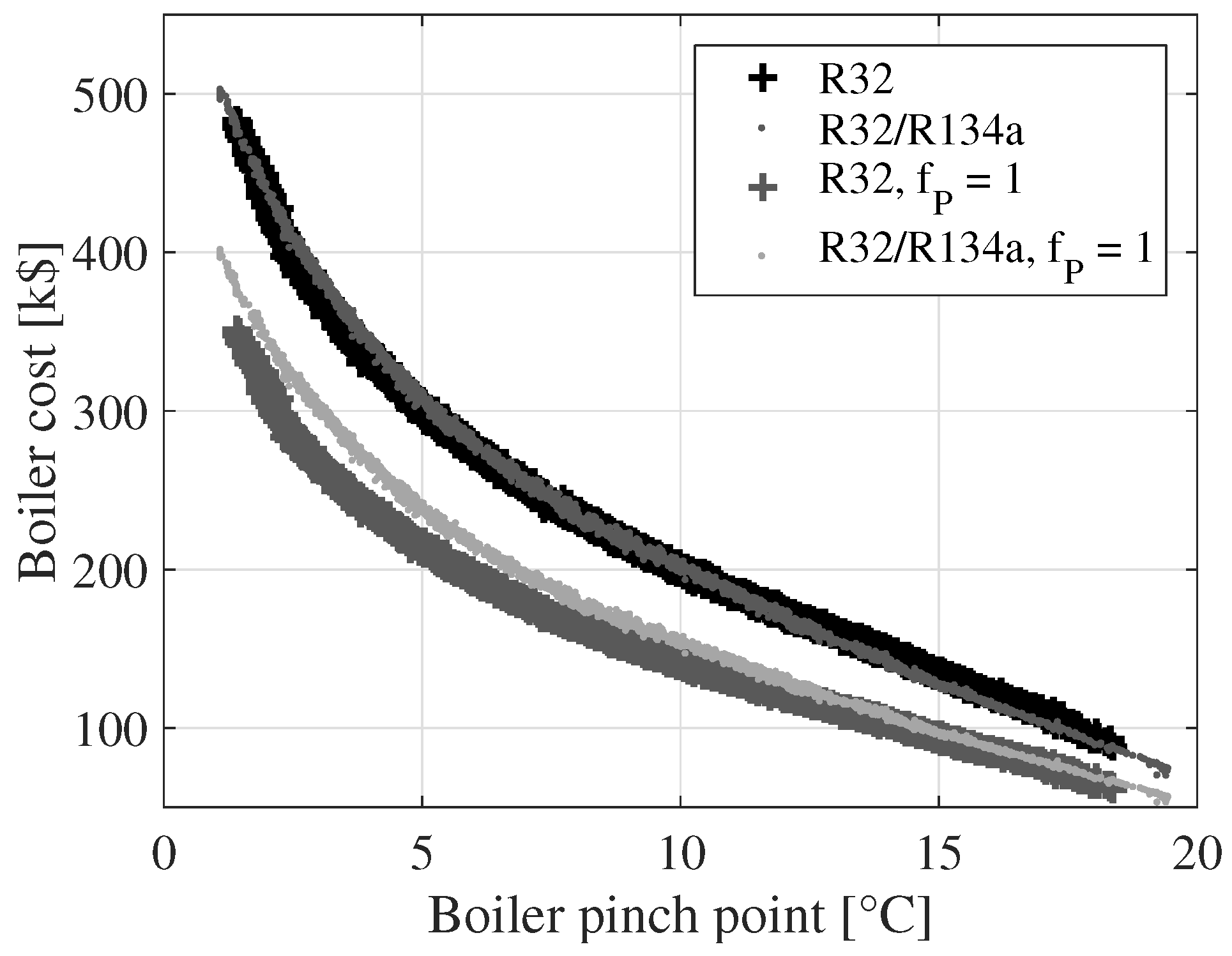
The boiler pressures range from 39–45 bar for R32, 28–35 bar for R32/R134a and 16–22 bar for R134a. Correspondingly, the critical pressures are 57.8 bar, 51.8 bar and 40.6 bar for R32, R32/R134a and R134a, respectively, thus indicating that higher critical pressures are related to higher optimum boiling pressures. Figure 10 displays a comparison of the boiler costs for R32 and R32/R134a with and without the pressure correction factor ($f_P$). The boiler pinch point is plotted on the x-axis. It is, thereby, possible to compare the boiler costs for a given pinch point temperature difference. When the pressure correction factor is unity, the boiler costs are higher for the mixture compared to R32. When the pressure correction factor is employed as a function of the boiler pressure, the boiler costs are similar for the two fluids. This indicates that the boiler pressure reduction, achieved when using the mixture, can compensate for the increase in boiler cost caused by the degradation of the heat transfer coefficient and the lower temperature difference of heat transfer.

For R32/R134a, the shell length to diameter ratio of the shell-and-tube heat exchangers are in a range of 37–110 for the condenser and 76–180 for the boiler. Shah and Sekulić [25] advise a desirable range of 3-15 for this ratio, meaning that the condensers and the boilers should consist of numerous shorter shell-and-tube heat exchangers in series, in order not to violate this practical limit. The shells designed in this paper are long since the number of tubes must be relatively low in order to ensure reasonable flow velocities in the tubes. Selecting a heat exchanger layout with multiple tube passes is a viable solution for increasing the number of tubes while maintaining high flow velocities in the tubes. Another option is to place the working fluid in the shell rather than in the tubes. This would increase the risk of working fluid leakage, which is problematic in the case of zeotropic mixtures.

4. Conclusions

This paper presents the results from a multi-objective optimization of net power output and component cost for ORC power plants using R32, R134 and R32/R134a (0.65/0.35${}_{\mathrm{mole}}$). For a low-temperature heat source, the results indicate that R32/R134a (0.65/0.35) is the best fluid and that R134a performs worst. For a total cost of 1200 k$, the mixture reaches 3.4% higher net power than R32 and 10.9% higher than R134a. The relative increase in net power output for the mixture compared to R32 is significantly lower than the 13.8%, which was estimated in a single-objective optimization of net power, i.e., not considering the cost of the cycle components. This exemplifies the importance of accounting for economic criteria in ORC system optimizations and fluid comparisons. This is especially important when pure fluids and mixtures are compared due to the generally lower temperature difference of heat transfer and the degradation of heat transfer coefficients for zeotropic mixtures. Moreover, the differences in operating pressures can have a significant effect on the cost of the ORC power plant. It is thus possible to reduce the cost of the boiler by using R32/R134a as the working fluid compared to R32, since the optimum pressure is lower for the mixture.

Future work on this topic will include performance comparisons for a larger group of pure fluids and mixtures and an extension of the economic analysis enabling the estimation of payback periods and net present values, so that the more cost efficient working fluids can be identified. An uncertainty analysis, assessing the influence of the uncertainties related to heat transfer and equipment cost correlations, is also a topic for further investigation, especially in the light of the relatively small performance differences observed for R32 and R32/R134a. The work could also be expanded to consider a detailed working fluid selection based on the proposed methodology while including factors as the availability, cost and environmental properties of working fluids. Additionally, the effects of using zeotropic mixtures on the turbine and pump performances are relevant for further analyses.