A New Approach of Modeling an Ultra-Super-Critical Power Plant for Performance Improvement

Abstract

A suitable model of coordinated control system (CCS) with high accuracy and simple structure is essential for the design of advanced controllers which can improve the efficiency of the ultra-super-critical (USC) power plant. Therefore, with the demand of plant performance improvement, an improved T-S fuzzy model identification approach is proposed in this paper. Firstly, the improved entropy cluster algorithm is applied to identify the premise parameters which can automatically determine the cluster numbers and initial cluster centers by introducing the concept of a decision-making constant and threshold. Then, the learning algorithm is used to modify the initial cluster center and a new structure of concluding part is discussed, the incremental data around the cluster center is used to identify the local linear model through a weighted recursive least-square algorithm. Finally, the proposed approach is employed to model the CCS of a 1000 MW USC one-through boiler power plant by using on-site measured data. Simulation results show that the T-S fuzzy model built in this paper is accurate enough to reflect the dynamic performance of CCS and can be treated as a foundation model for the overall optimizing control of the USC power plant.

1. Introduction

Ultra-super-critical (USC) power plants have been widely developed during the past decade for their high efficiency and low emission. For a large-scale once-through boiler power plant, the boiler and turbine are controlled as a whole object and the coordinated control system (CCS) is adopted. Since the CCS of a USC power plant is a complicated multivariable system with severe nonlinearity and coupling, the advanced controllers should be selected to improve the control efficiency. However, the advanced controllers always need a simple and precise mathematical model to maintain their high performance [1]. Therefore, in order to improve the performance of a USC power plant, it is essential to build a model of CCS with high accuracy and simple structure. Unfortunately, this modeling problem has been addressed in few reports, and the appropriate identification methods still need to be deeply researched.

The CCS of a USC power plant is too complex to be built accurately by conventional linear modeling methods [2], so nonlinear identification methods need to be adopted. At present, there are a few nonlinear modeling methods developed for a USC power plant, such as neural network methods [3], dynamic mechanism modeling [4,5], and neuro-fuzzy network methods [6]. The models built by the above approach are precise, but the model structure and the algorithm itself are complex. The fuzzy model proposed by Takagi-Sugeno [7] provides an efficient way to describe nonlinear systems. Based on If-Then rules, the relationship between input and output can be easily presented [8]. Due to its excellent features, the T-S fuzzy model has attracted significant attention from many researchers.

The T-S fuzzy model mainly contains a premise part and consequent part. For the premise part, the structure identification is important because it determines the fuzzy rule numbers. In order to get the suitable structure of the premise part, the fuzzy clustering algorithms which can perfectly divide the fuzzy space and find vague boundaries have been widely adopted [9]. The most common fuzzy clustering method is the fuzzy c-mean (FCM) algorithm [10,11,12,13]. This method can accurately identify the cluster centers and radius of data when the suitable cluster number and weighted exponent are chosen. However, the cluster results always depend on the initial values which are specified manually. The cluster number of fuzzy c-regression models (FCRM) [14] is also selected manually. When the cluster number is changed to find the optimal value, the whole cluster process should run again and again, which will lead to heavy computational effort. In [15], an entropy-based fuzzy clustering method was proposed for reducing the computation load. In this algorithm, the entropy just needs to be calculated once in the searching process, and the data pairs which have minimum entropy will be selected as initial cluster centers. Unfortunately, the data pairs which are away from the center area will be included in the initial center, because they also have small entropy. Based on the above analysis, in order to achieve suitable the cluster centers and cluster numbers, the improved clustering algorithm deserve to be studied.

After getting the cluster centers and radius of the data, the parameters of conclusion part will be calculated by the parameter estimation method, such as subspace identification (SID) methods [1], orthogonal least square method [14], weighted recursive least-square algorithm [16], and so on. However, the structure of the concluding part was rarely discussed. Though the model built by the above-mentioned method has high precision, it cannot be directly used by the advanced controller-based on a linear model. Thus, the new structure of conclusion part should be expanded to fit the demand of advanced controllers.

In this paper, an improved T-S fuzzy model identification approach is proposed to model a 1000 MW USC power plant for performance improvement. Firstly, an improved entropy-based fuzzy clustering method is adopted. The cluster numbers and initial centers of this method are automatically determined by introducing the concepts of a decision-making constant and threshold [17]. Meanwhile, the edge data points will not be selected as cluster centers. Then, the learning algorithm is used to modify the initial cluster centers and premise parameters are determined by modified cluster centers and the radius of cluster size. After this, a new structure of the concluding part is discussed, the incremental data around the cluster centers are used to get the local linear model through a weighted recursive least-square algorithm. The model built under the new structure can be directly used by advanced controllers. Finally, the on-site measured data of the power plant is used to train and verify the T-S fuzzy model, and two other different sets of data are selected to test the universality of the model.

The paper is organized as follows. In the next section, the CCS of the USC power plant is briefly described. Section 3 shows the new structure of the T-S fuzzy model. Section 4 describes the specific parameter estimation method, including the improved entropy clustering algorithm and weighted recursive least-square algorithm. Simulation results are given in Section 5. Finally, some conclusions are drawn in Section 6.

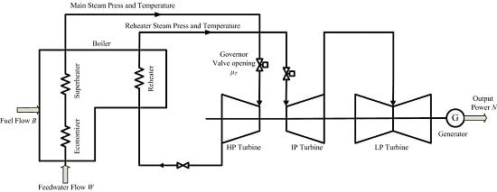
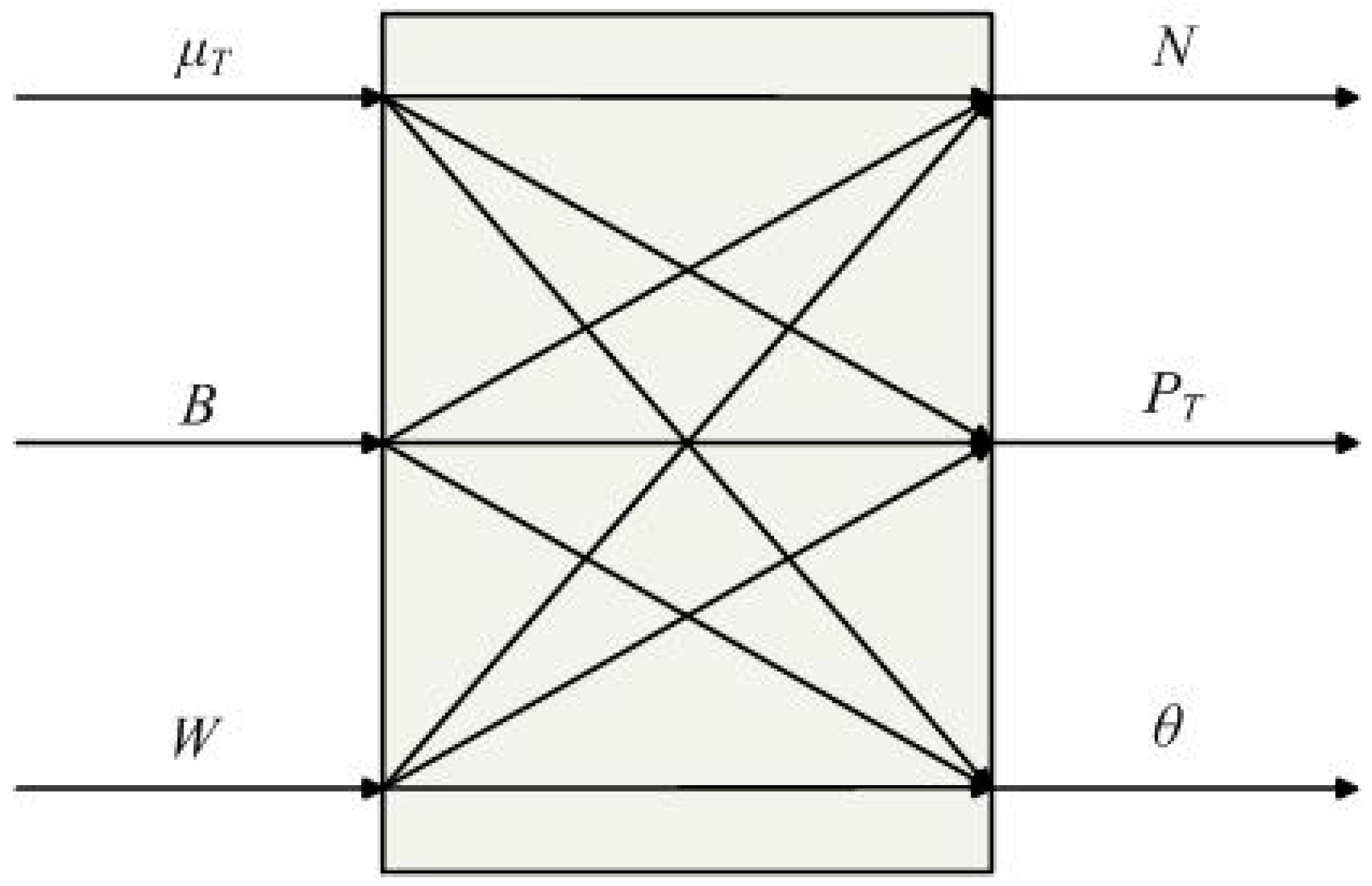
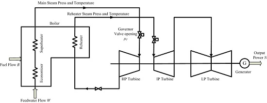
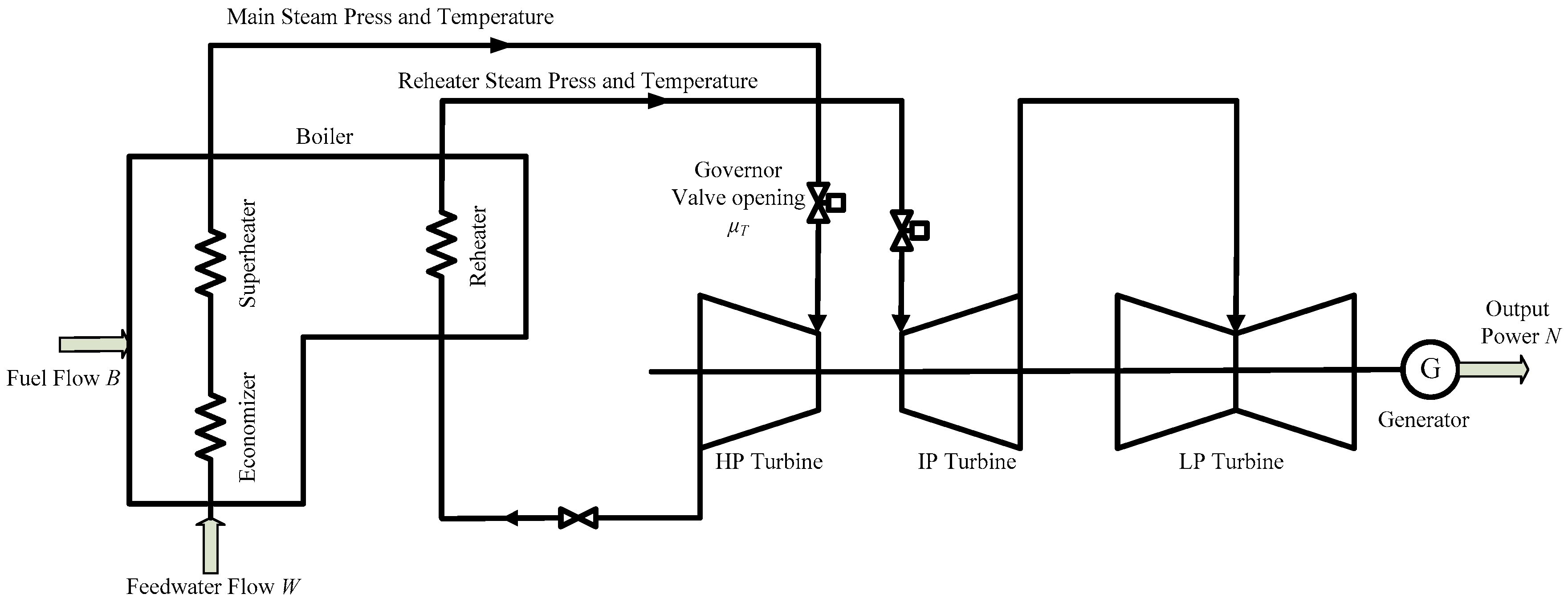
2. The Coordinated Control System of Ultra-Super-Critical Power Plant

When the steam parameters of a super-critical (SC) power plant reach 27 MPa/600 °C, it can be known as a USC power plant. Theoretical analysis indicated that the cycle heat efficiency of a USC power plant is 43%–49%, which is 10% higher than a sub-critical power plant. Due to its high efficiency, the USC power plant has become the leading fossil power generation unit around the world. The simplified structure of a USC power plant is shown in Figure 1.

At its critical state, water changes into steam instantly and there is no clear demarcation point between water and steam. The density of water is equal to steam, so the unit in the power plant cannot maintain natural circulation. In this case, the once-through boiler is adopted [18]. Compared with the sub-critical power plant, the USC power plant has the characteristics of strong coupling and nonlinearity, bringing challenges in modeling and control.

The structure of CCS in sub-critical power plants can usually be simplified as a double-input, double-output object [19], while it cannot accurately reflect the characteristics of a USC power plant. As the USC power plant does not use a drum boiler, the feed-water flow will directly affect the main steam pressure and unit power, and the control of fuel/water ratio is important for the safe operation of the unit. Hence, the feed-water flow and the separator outlet steam temperature, which reflect the fuel/water ratio, are selected as the manipulating variable and controlled variable, respectively. The CCS of a USC power plant can be modeled as a three-input, three-output nonlinear system, as shown in Figure 2.

In Figure 2, the outputs of CCS are the output power, the main steam pressure, and the separator outlet steam temperature. The inputs are the governor valve opening, the fuel flow and the feed-water flow, respectively. The new simplified structure can reflect the dynamics and key features of real power plant.

3. The New Structure of the T-S Fuzzy Model

3.1. Definition of New Structure

Takagi and Sugeno proposed an effective way to represent fuzzy models of nonlinear systems. A MIMO (multi-input, multi-output) system can be regarded as being made up of a series of multi-input, single-output (MISO) systems, and then suppose that a MISO system is the plant that needs to be considered.

Under the new structure, a MISO system can be described by the following fuzzy rules:

$$R^i:\mathrm{I}\mathrm{f}x\in (c_i,r_i)\mathrm{t}\mathrm{h}\mathrm{e}\mathrm{n}y{v}_i={\mathsf{\theta }}_i^{T}v,|i=1,2,\dots ,n$$

(1)

where $R^i$ is the ith rule, $n$ is the number of rules, $x$ is the input vector, $c_i$ and $r_i$ are the center and width of the membership function, $v$ is the incremental data vector of $x$, $y{v}_i$ is the output of the ith local linear model, and ${\mathsf{\theta }}_i$ is the conclusion parameter of the ith rule.

The input vector of the improved T-S model consists of all input variables and one output variable, and can be expressed as follows:

$$x_k={[u_1(k),\dots ,u_1(k-m_1),\dots ,u_p(k),\dots ,u_p(k-m_p),y(k),\dots ,y(k-\tau )]}^T$$

(2)

where $m_1,\cdots ,m_p$ are the order of different input variables, τ is the order of output variables. Correspondingly:

$$v_k={[\Delta u_1(k),\dots ,\Delta u_1(k-m_1),\dots ,\Delta u_p(k),\dots ,\Delta u_p(k-m_p),\Delta y(k),\dots ,\Delta y(k-\tau )]}^T$$

(3)

where

$$\begin{array}{l}\Delta u_j(k)=u_j(k)-us{t}_{ji}(j=1,\cdots ,p)\\ \Delta y(k)=y(k)-ys{t}_i\end{array}$$

(4)

$us{t}_{ji}(j=1,\cdots ,p)$ and $ys{t}_i$ are the static value of input vector which can get from $c_i$. For a nonlinear plant, the linear relationship only exists between $\Delta y$ and $\Delta u$, so v is used to identify the local linear model around $c_i$. $y{v}_i$ is the output of ith linear model, then the nonlinear output of the ith rule is calculated as follows:

$$y_i=y{v}_i+ys{t}_i$$

(5)

The final output of fuzzy model is:

$$y={\displaystyle \sum _{i=1}^n{w}_i{y}_i/{\displaystyle \sum _{i=1}^n{w}_i}}$$

(6)

where $w_i$ is the ith membership degree, and is generally calculated by the following equation:

$$\{\begin{array}{l}{w}_i=\exp (-\frac{\Vert x-c_i\Vert }{r_i}),\Vert x-c_i\Vert \le r_i\\ w_i=0,\Vert x-c_i\Vert >r_i\end{array}$$

(7)

The parameters $(c_i,r_i)$ are achieved from the training data. However, the training data is finite, this means trained regions cannot cover the entire input space, so there will exist a situation where new test data points do not belong to any rules $({\displaystyle \sum w_i=0})$, and Equation (6) cannot be calculated. To deal with this problem, an adaptive inference is adopted.

• Seek the clustering center $c_s$, which has the shortest distance between $x$ through Equation (8).

  $$\Vert x-c_s\Vert =\min \Vert x-c_i\Vert (i=1,2,\cdots ,n)$$

  (8)
• Calculate the output of local linear model.

  $$y{v}_s={\mathsf{\theta }}_s^{T}v$$

  (9)
• The final output of the fuzzy model is:

  $$y=y{v}_s+ys{t}_s$$

  (10)

The shortest distance means that the data is extremely similar, so using the dynamic parameter of $c_s$ to calculate the final output is reasonable.

3.2. Discussion of the New Structure

For the concluding part, there are two general kinds of structure:

$$y_i={\mathsf{\theta }}^T{x}_i+e_{i}i=1,\dots ,n$$

(11)

$$y_i=s_i+{\mathsf{\varphi }}^T{x}_{i}i=1,\dots ,n$$

(12)

Equation (11) is used in [14]. $e_i$ is the identification error, and the nonlinear data around the cluster center is used directly to get the local model. Equation (12) is used in [16]. The static parameters $s_i(i=1,\dots ,n)$ are obtained, firstly, and then the dynamic parameters $\mathsf{\varphi }$ are calculated. However, input vectors $x_i(i=1,\dots ,n)$ still use nonlinear data. For a nonlinear system, the linear relationship exists between Δy and Δu. In addition, the concluding parameters of these two structures are totally different for the same plant. Hence, the models built by above structures cannot be applied in designing linear controllers.

In general, the local linear model of a nonlinear system can be obtained at the typical operating point through the incremental data. In order to guarantee the high precision of the linear model, the initial data must be limited to a small range for it cannot include nonlinear components.

Based on the above analysis, this paper treats the cluster center as the operating point, and then the incremental data around the cluster center is employed to get the local linear model. This approach can get rid of the limit of initial data, which means the global data can be used directly. The model built under the new structure can be described as a linear time-varying model. In each sampling period, a group of system variables can be obtained, then the membership degree will be calculated through antecedent part. After that, the linear model which is suitable for the current moment will be achieved. It is easy to take advantage of abundant advanced control theories to design control systems. Hence, the approach proposed in this paper provides a foundation model for the overall optimizing control of the USC power plant.

4. Parameters Estimation

4.1. Definition of Entropy

The input vector used for identify is $x_k(k=1,\cdots ,N)$, the entropy can be calculated by the following equation:

$$\begin{array}{l}{E}_{ij}=S_{ij}{\log }_2{S}_{ij}+(1-S_{ij}){\log }_2(1-S_{ij})\\ E_i=-{\displaystyle \sum _{\begin{array}{l}j=1\\ j\ne i\end{array}}^N{E}_{ij}}\end{array}$$

(13)

In Equation (13), when S_ij is close to 0 or 1, the value of E_ij is small (close to 0), when S_ij = 0.5, E_ij is equal to 1, S_ij is the similarity between the input vector x_i and x_j, which can be calculated by the following equation:

$$\begin{array}{c}{S}_{ij}=e^{-\alpha D_{ij}}\\ D_{ij}=\Vert x_i-x_j\Vert \end{array}$$

(14)

where i = 1, 2, ..., N, j = 1, 2, ..., N, D_ij is the Euclidean distance between x_i and x_j. The maximum and minimum of similarity for the input vector $x_i$ are $S_{i\max }$ and $S_{i\min }$, then normalize the similarity through Equation (15).

$$S_{ij}=\frac{S_{ij}-S_{i\min }}{S_{i\max }-S_{i\min }}$$

(15)

The range of normalized S_ij is [0, 1]. When the distance between two data pairs is small, the value of similarity is close to 1. Correspondingly, when the value of similarity is close to 0, it means that the distance between the two data pairs is large.

4.2. Improved Entropy Clustering Algorithm

In the conventional entropy clustering algorithm [15], the data points which have minimum entropy will be taken as initial cluster centers. However, the cluster centers will contain edge data pairs for they also have small entropy. In order to solve this problem, an improved entropy clustering algorithm is proposed by introducing the concepts of decision-making constant [17] and threshold. The specific implementation process is as follows:

• Calculate the entropy $E_k(k=1,\cdots ,N)$ according to the $N$ input training data pairs $x_k(k=1,\cdots ,N)$ and initialize the cluster number $n=1$.
• The input vector x_s which has the smallest entropy $E_s=\min (E_k)$ is selected as the cluster center c_n. Then calculate similarity S_ij between input data pairs x_k (k = 1, 2, ..., N) and c_n, the total number of data pairs which meet $S(x_k,c_n)>\mathsf{\beta }$ is NC. β is the decision-making constant; it decides whether the data pairs x_k belong to the same class with the cluster center.
• Introduce the threshold va. If $NC>va$, accepting $c_n$ as the initial cluster center, go to step 4. If $NC<va$, refusing $c_n$ as the initial cluster center, then $x_s$ and $E_s$ are removed from $x_k$ and $E_k$, respectively, $N=N-1$ and go step 2. This step can avoid selecting the isolated data pairs as cluster center.
• Remove the data pairs which meet $S(x_k,c_n)>\mathsf{\beta }$ from initial training data.
• The number of remaining data is $N=N-NC$. If $N<va$, the cluster of data is finished and $c_i(i=1,\cdots ,n)$ is taken as the initial cluster centers. If $N>va$, $n=n+1$, return to step 2.

4.3. Cluster Center Modification

According to the above algorithm, the initial cluster centers can be achieved, but some of the training data pairs are not classified (isolated data and the last remaining data), in order to guarantee integral data, the learning algorithm is used to modify the cluster centers.

• Through the above clustering, the initial cluster center $c_i(i=1,\cdots ,n)$ can be achieved.
• Select any input data vector $x_k$ from training data pairs, and find out the nearest cluster center by Equation (16):

  $$\Vert x_k-c_s\Vert =\min \Vert x_k-c_i\Vert ,(i=1,\dots ,n)$$

  (16)
• Using $x_k$ to update the cluster center $c_s$:

  $$\begin{array}{l}{n}_s=n_s+1\\ c_s=c_s+{\alpha }_c(x_k-c_s)\end{array}$$

  (17)

  where ${\alpha }_c$ is the learning rate, ${\alpha }_c<1$ and gradually decay to 0:

  $${\alpha }_c=\frac{1}{n_s}$$

  (18)
• Select another input vector from the training data and repeat steps 2 and 3, then the revised cluster centers can be obtained.

4.4. Identification of Cluster Radius

After obtaining the cluster centers, the radius of the cluster center can be ensured according to following algorithm:

• The initial value of radius is set to r_i = 0 (i = 1, 2, …, n). Select an input vector $x_k$ and find the nearest cluster center $c_s$:

  $$\Vert x_k-c_s\Vert =\min \Vert x_k-c_i\Vert ,(i=1,\cdots ,n)$$

  (19)
• Update $r_s$ through the following equation:

  $$r_s=\max \left\{\Vert x_k-c_s\Vert ,r_s\right\}$$

  (20)
• Repeating steps 1 and 2, the cluster radius $r_i(i=1,\dots ,n)$ can be obtained.

4.5. Identification of the Concluding Parameters

As described above, the concluding parameters to improve the T-S fuzzy model is the relationship between $yv$ and $v$, so before calculating the dynamic concluding parameter, the training data pairs $x_k(k=1,\dots ,N)$ should be preprocessed. Then, the exponentially-weighted least squares method is employed to obtain the linear dynamic parameters.

• Initialize matrix $P_i(i=1,\dots ,n),P_i=\alpha I,\alpha ={10}^6$, $I$ is the identity matrix.
• Select the training data pairs $(x_k,y_k)$, where $x_k$ is the input vector, $y_k$ is the output, and the dynamic parameters ${\mathsf{\theta }}_i(i=1,\dots ,n)$ can be calculated through Equation (21).

  $$\begin{array}{ll}\mathrm{If}\hfill & \Vert x_k-c_i\Vert \le r_i\begin{array}{c}\end{array}\mathrm{then}\hfill \\ & v_k=x_k-c_i\hfill \\ & y{v}_k=y_k-ys{t}_i\hfill \\ & P_i(t+1)=\frac{1}{{\lambda }_i(t)}\left\{P_i(t)-\frac{P_i(t)v_k{v}_k^T{P}_i(t)}{{\lambda }_i(t)+Q+v_k^T{P}_i(t)v_k}\right\}\hfill \\ & {\mathsf{\theta }}_i(t+1)={\mathsf{\theta }}_i(t)+P_i(t+1)(y{v}_k-v_k^T{\mathsf{\theta }}_i(t))v_k\\ & {\lambda }_i(t)={\lambda }_0{\lambda }_i(t-1)+1-{\lambda }_0{\lambda }_0=0.6\\ \mathrm{If}& \Vert x_k-c_i\Vert >r_i\begin{array}{c}\end{array}\mathrm{then}\\ & P_i(t+1)=P_i(t)\\ & {\mathsf{\theta }}_i(t+1)={\mathsf{\theta }}_i(t)\end{array}$$

  (21)

  $ys{t}_i$ is the static value of output which can get from $c_i$. $Q$ can be calculated through $Q=\exp (-t/m)$, m is a positive integer, in this paper, and $m$ is set to 50.
• t = t + 1, and return to step 2; after all training data have been used, the dynamic parameters of the concluding part can be obtained.

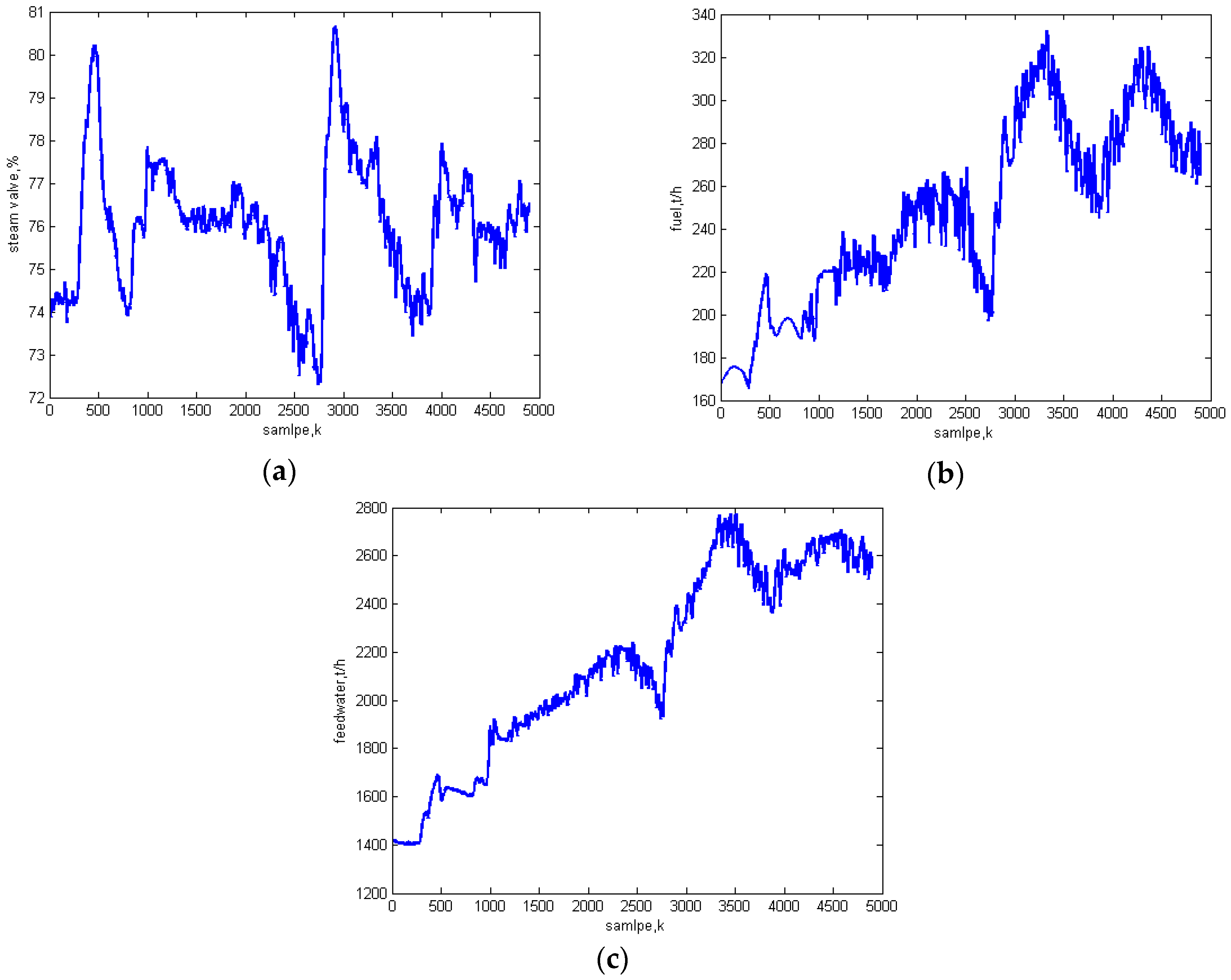
5. Simulation

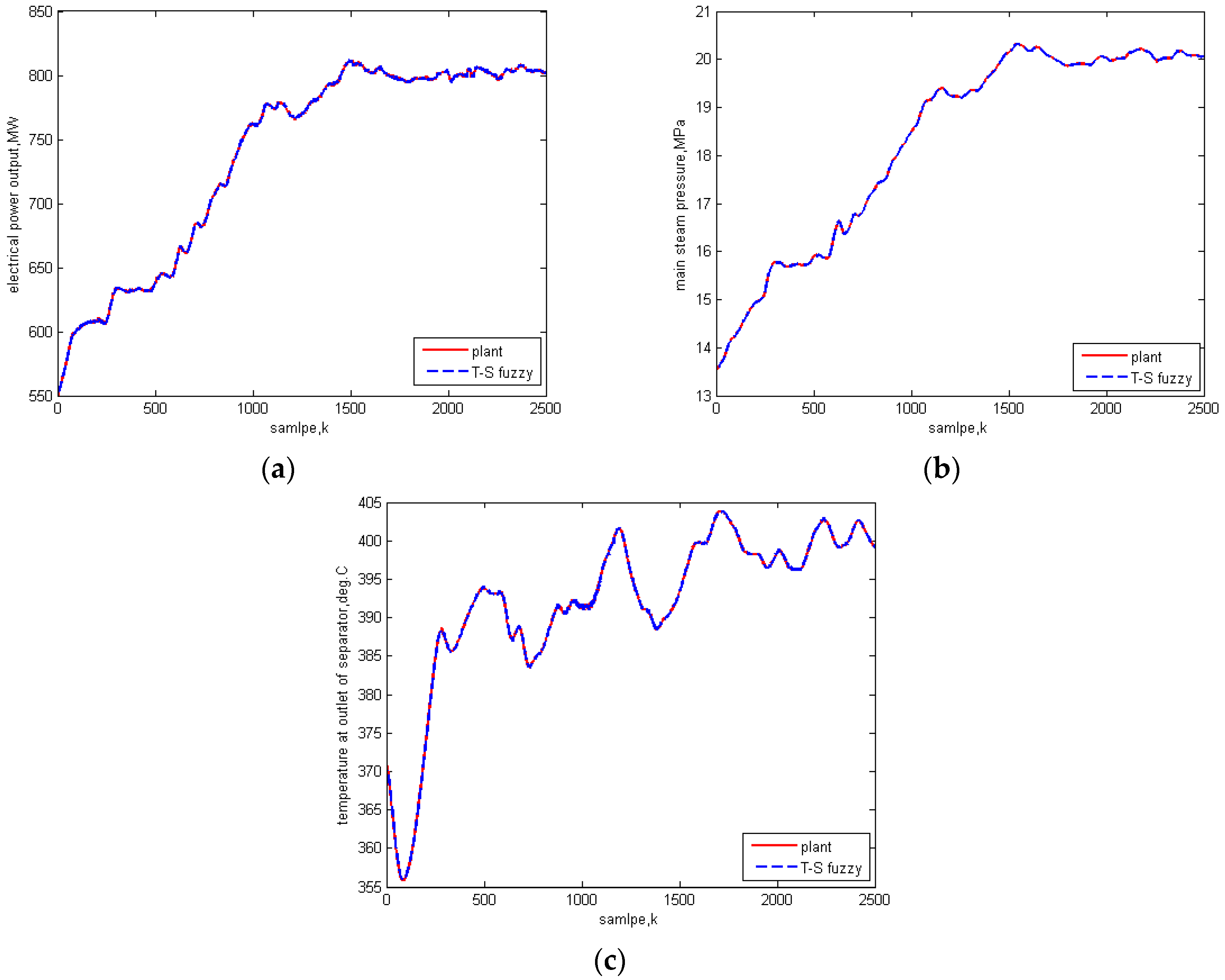
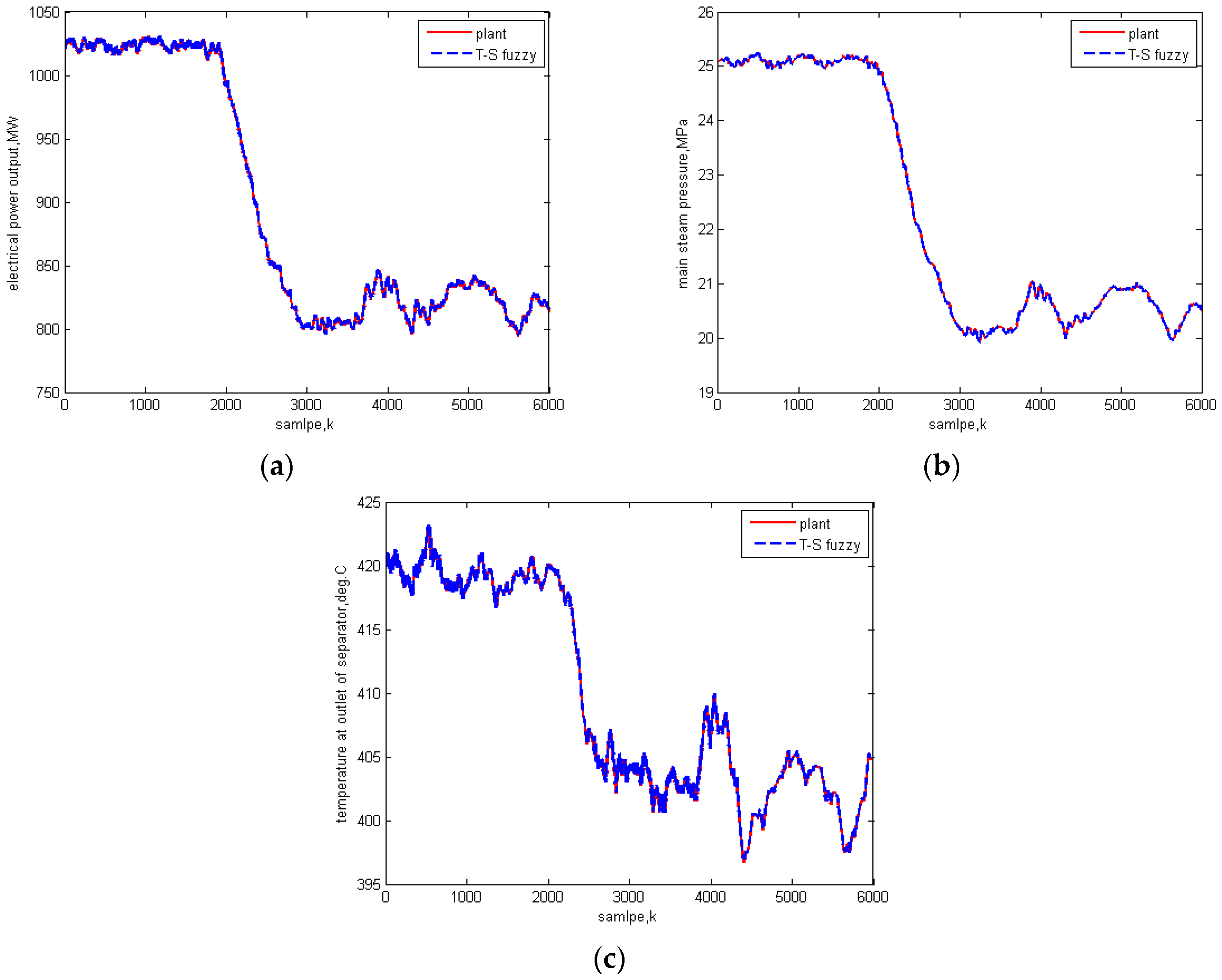
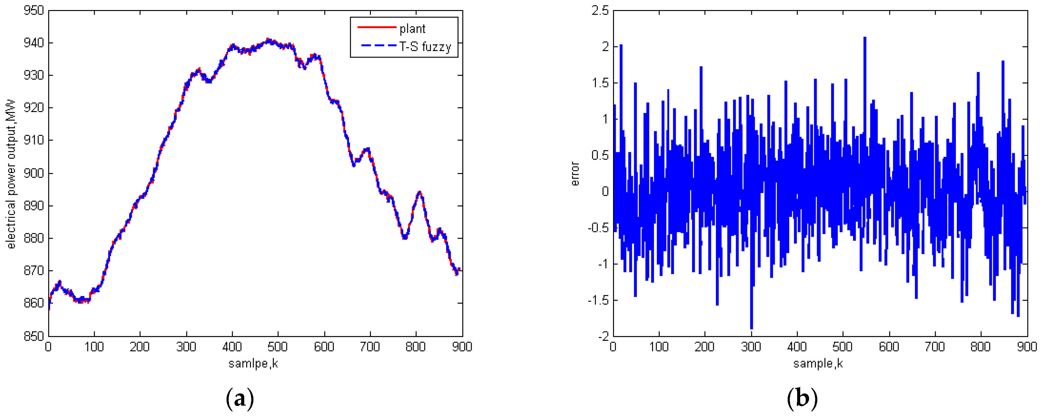
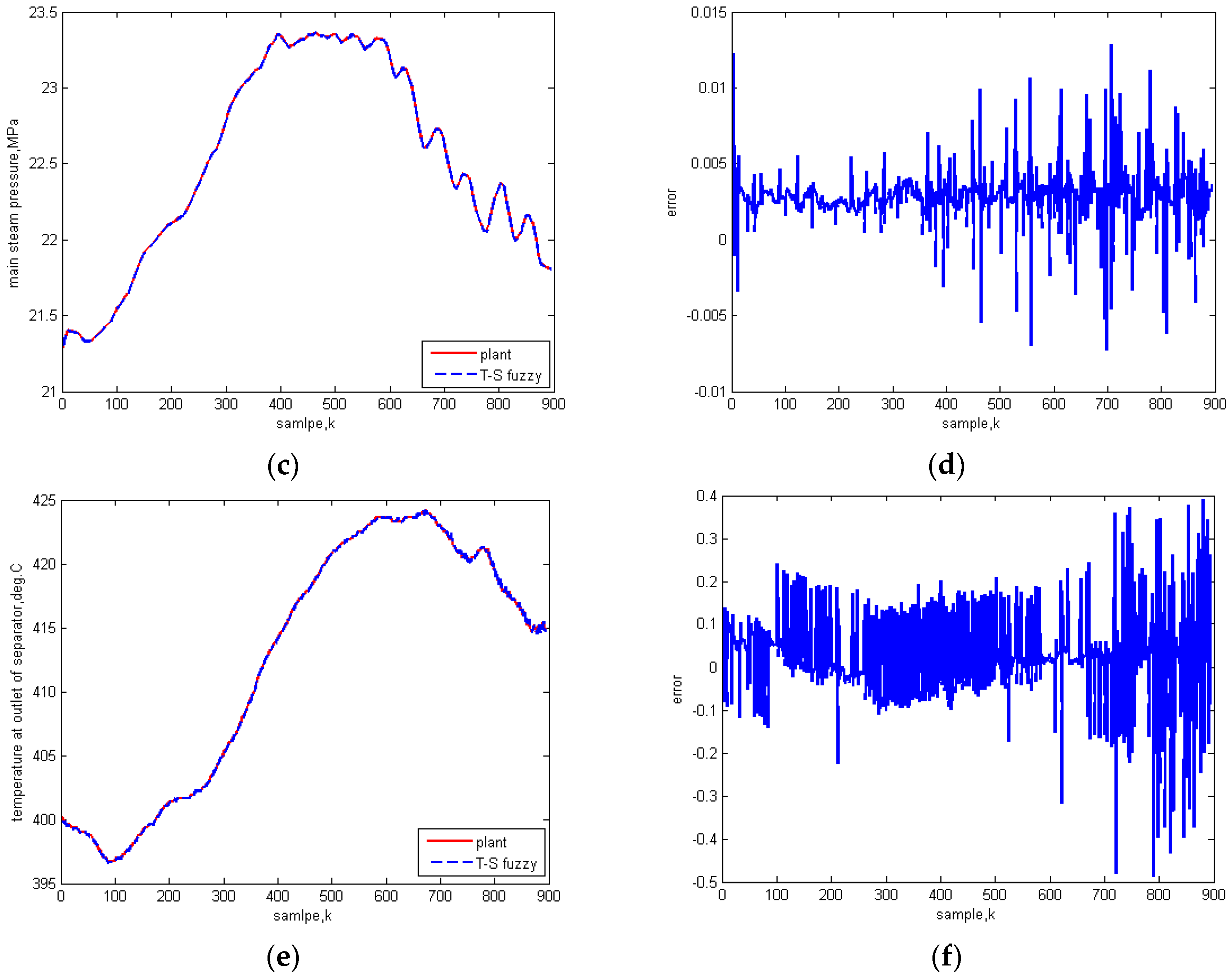
5.1. Identification Results

The on-site measured data of the 1000 MW USC power plant is used to test the validity of the proposed algorithm. 4900 sets of data are selected for identification, in which load is changed from 500 to 1000 MW and the sampling time is three seconds. The input data of CCS is shown in Figure 3.

The first 4000 are treated as training data, and the rest 900 as test data. The CCS contains three inputs and three outputs, so it can be divided into three MISO system, the input vectors are selected as follows:

$$\begin{array}{c}{x}_{k1}(k)=\left(\begin{array}{l}{u}_1(k),\dots ,u_1(k-m_1),u_2(k),\dots ,u_2(k-m_2),\\ u_3(k),\dots ,u_3(k-m_3),y_1(k),\dots ,y_1(k-\tau )\end{array}\right)\\ x_{k2}(k)=\left(\begin{array}{l}{u}_1(k),\dots ,u_1(k-m_1),u_2(k),\dots ,u_2(k-m_2),\\ u_3(k),\dots ,u_3(k-m_3),y_2(k),\dots ,y_2(k-\tau )\end{array}\right)\\ x_{k3}(k)=\left(\begin{array}{l}{u}_1(k),\dots ,u_1(k-m_1),u_2(k),\dots ,u_2(k-m_2),\\ u_3(k),\dots ,u_3(k-m_3),y_3(k),\dots ,y_3(k-\tau )\end{array}\right)\end{array}$$

(22)

where $m_1=m_2=m_3=\mathsf{\tau }=3$, the order of input vectors are the same as in [6]. Then, there are two parameters need to be ensured: β and $va$. Firstly, changing the value of β while maintaining $va=0.004N$. Then, the suitable value of β can be ascertained through the cluster number and identification accuracy.

In this paper, the mean square error (MSE) is selected as the performance index of the fuzzy model, which can be calculated as follows:

$$\delta =\frac{1}{N}{\displaystyle \sum _{k=1}^N{(y_k-{\tilde{y}}_k)}^2}$$

(23)

where $y_k$ is real output, ${\tilde{y}}_k$ is identified output, $N$ is the number of training data.

As shown in

Table 1. Comparison of different β for different objects while va remains unchanged.

(a) Comparison of different β for electrical power output while va = 0.004N	β	Cluster Number	MSE
	0.5	20	0.0087
	0.6	12	0.0097
	0.65	4	0.0123
	0.7	2	0.0260
(b) Comparison of different β for the main steam pressure while va = 0.004N	β	Cluster Number	MSE
	0.6	13	4.2561 × 10−5
	0.65	7	1.1322 × 10−4
	0.7	5	7.3223 × 10−5
	0.75	3	2.8506 × 10−4
(c) Comparison of different β for the separator outlet steam temperature while va = 0.004N	β	Cluster Number	MSE
	0.5	28	0.0016
	0.6	11	0.0017
	0.65	5	0.0018
	0.7	3	0.0024

, the identification accuracy changes little while the cluster numbers varying in a large range. Thus, in this paper, the best cluster numbers are chosen close to the number of typical working-points of plant. For USC power plant, the number can be chosen from 3 to 5.

Select β = 0.65 for load model, β = 0.7 for main steam pressure model and β = 0.65 for temperature at outlet of separator model, then change the value of $va$.

From

Table 2. Comparison of different va for different objects while β remains unchanged.

(a) Comparison of different va for electrical power output while β = 0.65	va	Cluster Number	MSE
	0.002N	25	0.0084
	0.003N	9	0.0098
	0.004N	4	0.0123
	0.005N	2	0.0248
(b) Comparison of different va for the main steam pressure while β = 0.7	va	Cluster Number	MSE
	0.002N	23	4.1539 × 10−5
	0.003N	8	4.8359 × 10−5
	0.004N	5	7.3223 × 10−5
	0.005N	3	7.1348 × 10−5
(c) Comparison of different va for separator outlet steam temperature while β = 0.65	va	Cluster Number	MSE
	0.002N	34	0.0037
	0.003N	15	0.0017
	0.004N	5	0.0018
	0.005N	4	0.0019

, it can be seen that the change of $va$ can also have great effect on the cluster number. According to the analysis of the preceding context, the best cluster numbers can be chosen from 3–5. So the value of $va$ can be selected as 0.004N for load model, 0.004N for the main steam pressure model and 0.004N for separator outlet steam temperature model. After this, the improved T-S fuzzy identification algorithm is applied to CCS. The parameters of the T-S fuzzy model are listed in Appendix A. The output comparison between the T-S fuzzy model and training data is shown in Figure 4.

From the figure it could be seen that the training model has great approximation capability. Then, the test data are used to verify the right of training model, Figure 5 shows the comparison between T-S fuzzy model and test data. Simulation results show that the training model is suitable for test data.

5.2. Comparison Test

Three different modeling methods are compared to show the identification precision, and the MSE values are listed in

Table 3. MSE of different methods for different models.

Methods	Power Model	Pressure Model	Temperature Model
ARX model [2]	0.1058	0.0026	0.0964
Original T-S [16]	0.0705	0.0012	0.0233
Proposed method	0.0123	7.3223 × 10−5	0.0018

. The autoregressive exogenous (ARX) model can be easily used by advanced controllers, but it cannot accurately reflect the whole dynamic feature of USC power plant. From

Table 4. Number of rules.

Methods	Power Model	Pressure Model	Temperature Model
Original T-S	6	4	4
Proposed method	4	5	5

, it can be seen that the cluster numbers of the original fuzzy model and the proposed method are similar. However, the precision of the original fuzzy model is not high enough due to using nonlinear data directly. For the USC power plant, the amplitude of input data is high. It is hard to obtain the linear model using nonlinear data around each cluster center. Thus, the original fuzzy model is not suitable for the USC power plant. The new method proposed in this paper has high accuracy and it provides useful information to improve the design of the advanced controller for the USC power plant. Meanwhile, the performance of the USC power plant can be further improved.

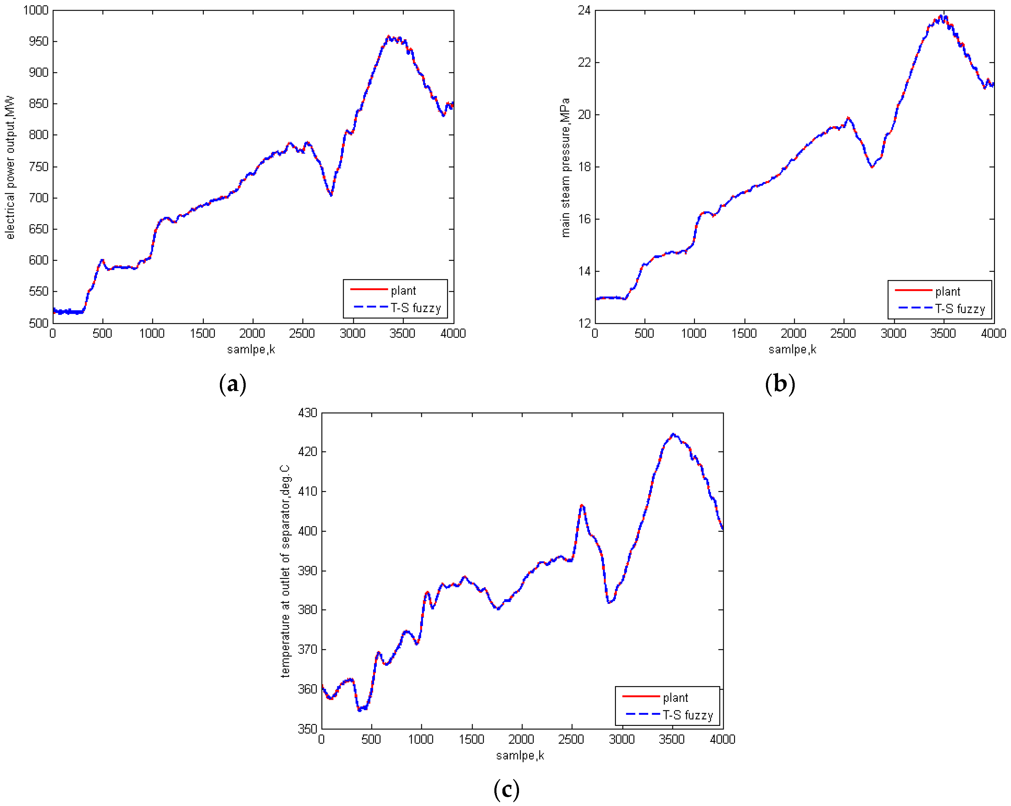
5.3. Universality Test

In order to verify the universality of the T-S fuzzy model, another two sets of data are selected. The new test data are the real-time data of the power plant at different day and different timeframes, which have no relation with the data used in the last section. If the model still has high identification precision, the universality of the T-S fuzzy model can be proved.

The load of the first set of data is ranging from 550 to 800 MW, and the other is changing from 1025 to 800 MW. Figure 6 shows the comparison between the T-S fuzzy model and the new test data 1. The comparison between the T-S fuzzy model and the new test data 2 is presented in Figure 7. From the simulation results, it can be concluded that the fuzzy models built in this paper have good robustness and can represent the feature of 1000 MW USC power plant.

6. Conclusions

In order to get a suitable mathematical model of the 1000 MW USC one-through boiler power plant for performance improvement, an improved T-S model identification approach is presented in this paper. The improved entropy cluster algorithm is applied to identify the premise parameters. By introducing the concept of decision-making constant and threshold, the cluster number and initial centers can be automatically determined. After this, the learning algorithm is used to modify the initial cluster centers, and a new structure of the concluding part is proposed. For the purpose of getting a more precise local linear model, the incremental data around the cluster center is selected and the weighted recursive least-square algorithm is used to estimate the parameters. Finally, the on-site measured data of USC power plant is used to build the model and test the universality of the model. From the simulation results, it can be concluded that the proposed approach has great approximation capability and the T-S fuzzy model built in this paper can represent the feature of USC power plant. Due to the new structure, the model can also be seen as a foundation model for the overall optimizing control of the USC power plant.

References

1. Wu, X.; Shen, J.; Li, Y.G.; Lee, K.Y. Data-driven modeling and predictive control for boiler-turbine unit using fuzzy clustering and subspace methods. ISA Trans. 2014, 53, 699–708. [Google Scholar] [CrossRef] [PubMed]
2. Ding, J.; Li, G.Y.; Wang, N. Research on simplified model for the control of 660 MW supercritical unit. Electr. Power Sci. Eng. 2011, 27, 29–34. [Google Scholar]
3. Lee, K.Y.; Van Sickel, J.H.; Hoffman, J.A.; Jung, W.H.; Kim, S.H. Controller design for a large-scale ultrasupercritical once-through boiler power plant. IEEE Trans. Energy Convers. 2010, 25, 1063–1070. [Google Scholar] [CrossRef]
4. Wei, J.L.; Wang, J.H.; Wu, Q.H. Development of a multi-segment coal mill model using an evolutionary computation technique. IEEE Trans. Energy Convers. 2007, 22, 718–727. [Google Scholar] [CrossRef]
5. Yan, S.; Zeng, D.L.; Liu, J.Z.; Liang, Q.J. A simplified non-linear model of a once-through boiler-turbine unit and its application. Chin. Soc. Electr. Eng. 2012, 32, 126–134. [Google Scholar]
6. Liu, X.J.; Kong, X.B.; Hou, G.L.; Wang, J.H. Modeling of a 1000 MW power plant ultra super-critical boiler system using fuzzy-neural network methods. Energy Convers. Manag. 2013, 65, 518–527. [Google Scholar] [CrossRef]
7. Takigi, T.; Sugeno, M. Fuzzy identification of system and its application to modeling and control. IEEE Trans. Syst. Man Cybern. 1985, 15, 116–132. [Google Scholar] [CrossRef]
8. Chakrborty, D.; Pal, N.R. Integrated feature analysis and fuzzy rule-based system identification in a neuro-fuzzy paradigm systems. IEEE Trans. Syst. Man Cybern. 2001, 31, 391–400. [Google Scholar] [CrossRef] [PubMed]
9. Frank, K.; Rudoif, K.; Roland, W. Fuzzy clustering: More than just fuzzification. Fuzzy Sets Syst. 2015, 281, 272–279. [Google Scholar]
10. Wang, N.; Yang, Y.P. A fuzzy modeling method via Enhanced Objective Cluster Analysis for designing TSK model. Expert Syst. Appl. 2009, 36, 12375–12382. [Google Scholar] [CrossRef]
11. Zhang, B.J.; Qin, S.; Wang, W.; Wang, D.; Xue, L. Data stream clustering based on fuzzy c-mean algorithm and entropy theory. Signal Process. 2015, 1–6. [Google Scholar] [CrossRef]
12. Zhang, J.A.; Jia, M.P. Segmentation algorithm for small targets based on improved data field and fuzzy c-means clustering. Optik 2015, 126, 4330–4336. [Google Scholar]
13. Kannan, S.R.; Ramathilagam, S.; Chung, P.C. Effective fuzzy c-means clustering algorithms for data clustering problems. Expert Syst. Appl. 2012, 39, 6292–6300. [Google Scholar] [CrossRef]
14. Li, C.S.; Zhou, J.Z.; Li, Q.Q. A new T-S fuzzy-modeling approach to identify a boiler-turbine system. Expert Syst. Appl. 2010, 37, 2214–2221. [Google Scholar] [CrossRef]
15. Shimoji, S.; Lee, S. Data clustering with entropic scheduling. In Proceeding of the IEEE Conference on Fuzzy Systems, Orlando, FL, USA, 26–29 June 1994; pp. 2423–2428.
16. Hou, G.L.; Hou, Q.; Zhang, J.H. T-S Fuzzy modeling based on compatible relation and its application in power plant. In Proceeding of the IEEE Conference on Industrial Electronics and Applications, Beijing, China, 21–23 June 2011; pp. 1308–1313.
17. Yao, J.; Dash, M.; Tan, S.T.; Liu, H. Entropy-based fuzzy clustering and fuzzy modeling. Fuzzy Sets Syst. 2000, 113, 381–388. [Google Scholar] [CrossRef]
18. Ma, L.Y.; Kwang, Y.L.; Wang, Z.Y. Intelligent coordinated controller design for a 600 MW supercritical boiler unit based on expanded-structure neural network inverse models. Control Eng. Pract. 2015, 9, 1–8. [Google Scholar] [CrossRef]
19. Han, Z.X.; Zhang, Z.; Qi, X.H. Analysis of linear increment mathematic model for multivariate boiler-turbine coordinated control object. Chin. Soc. Elec. Eng. 2005, 25, 24–29. [Google Scholar]
Figure 1. Schematic diagram for an ultra-super-critical (USC) power plant.
Energies 09 00310 g001
Figure 2. Coordinated control system (CCS) of a USC power plant.
Energies 09 00310 g002
Figure 3. (a) Data of steam valve degree of opening; (b) Data of fuel; (c) Data of the feed-water flow.
Energies 09 00310 g003
Figure 4. (a) Comparison of the T-S fuzzy model and training data for electrical power output; (b) Comparison of the T-S fuzzy model and training data for main-steam pressure; (c) Comparison of the T-S fuzzy model and training data for the separator outlet steam temperature.
Energies 09 00310 g004
Figure 5. (a) Comparison of the T-S fuzzy model and test data for electrical power output; (b) validation error of the load model; (c) comparison of the T-S fuzzy model and test data for main-steam pressure; (d) validation error of main-steam pressure model; (e) comparison of the T-S fuzzy model and the test data for the separator outlet steam temperature; and (f) validation error of the separator outlet steam temperature model.
Energies 09 00310 g005aEnergies 09 00310 g005b
Figure 6. (a) Comparison of the T-S fuzzy model and new test data 1 for electrical power output; (b) Comparison of T-S fuzzy model and new test data 1 for main-steam pressure; (c) Comparison of T-S fuzzy model and new test data 1 for the separator outlet steam temperature.
Energies 09 00310 g006
Figure 7. (a) Comparison of T-S fuzzy model and new test data 2 for electrical power output; (b) Comparison of the T-S fuzzy model and new test data 2 for main-steam pressure; (c) Comparison of T-S fuzzy model and new test data 2 for the separator outlet steam temperature.
Energies 09 00310 g007