
Distributed Energy Storage Using Residential Hot Water Heaters


Abstract
:1. Introduction
2. System Description and Methodology
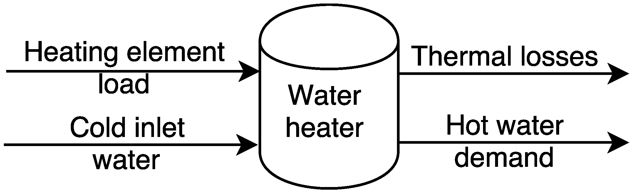
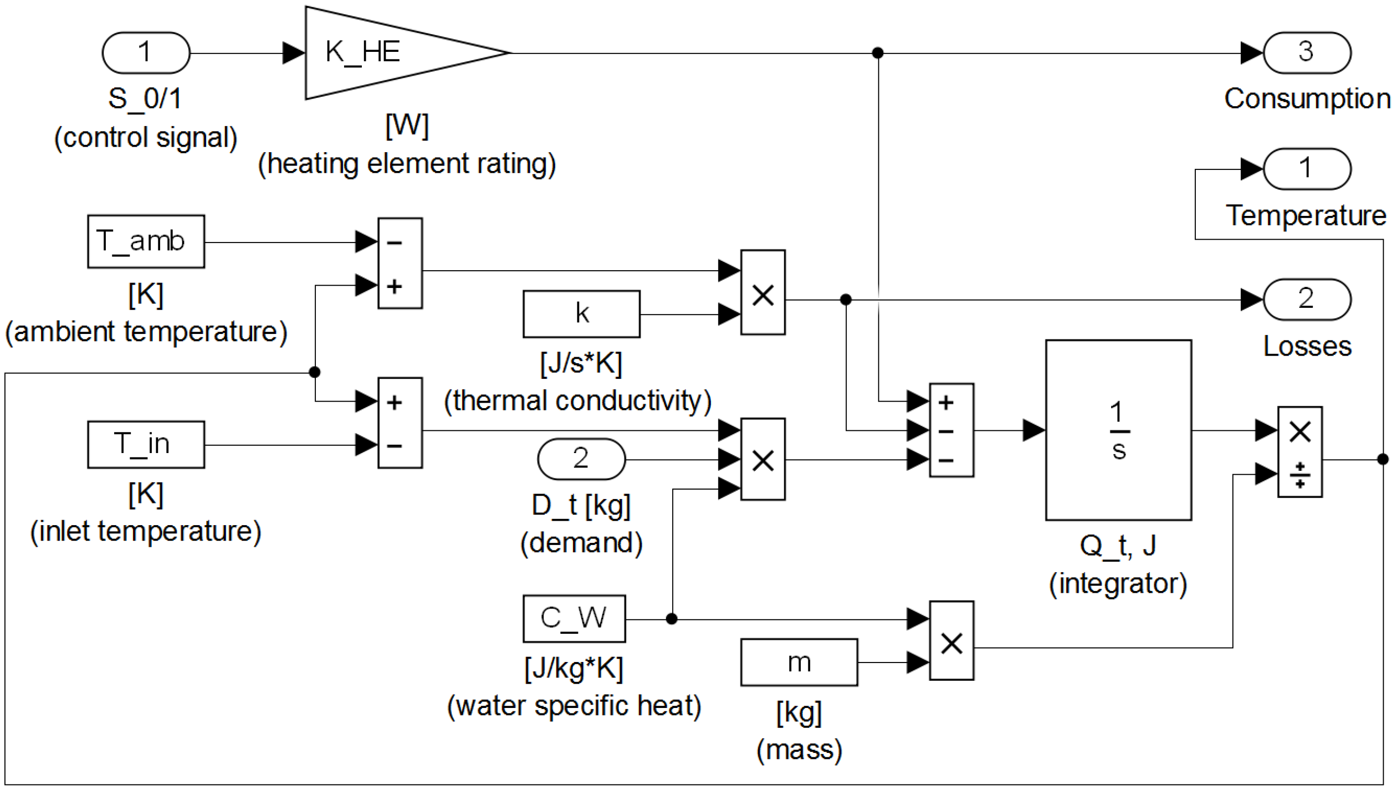
2.1. Thermal Water Heater Model
2.2. Smart Hot Water Heater Controller
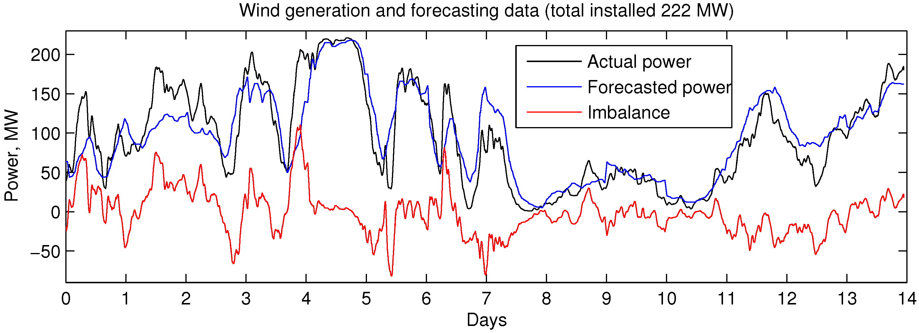
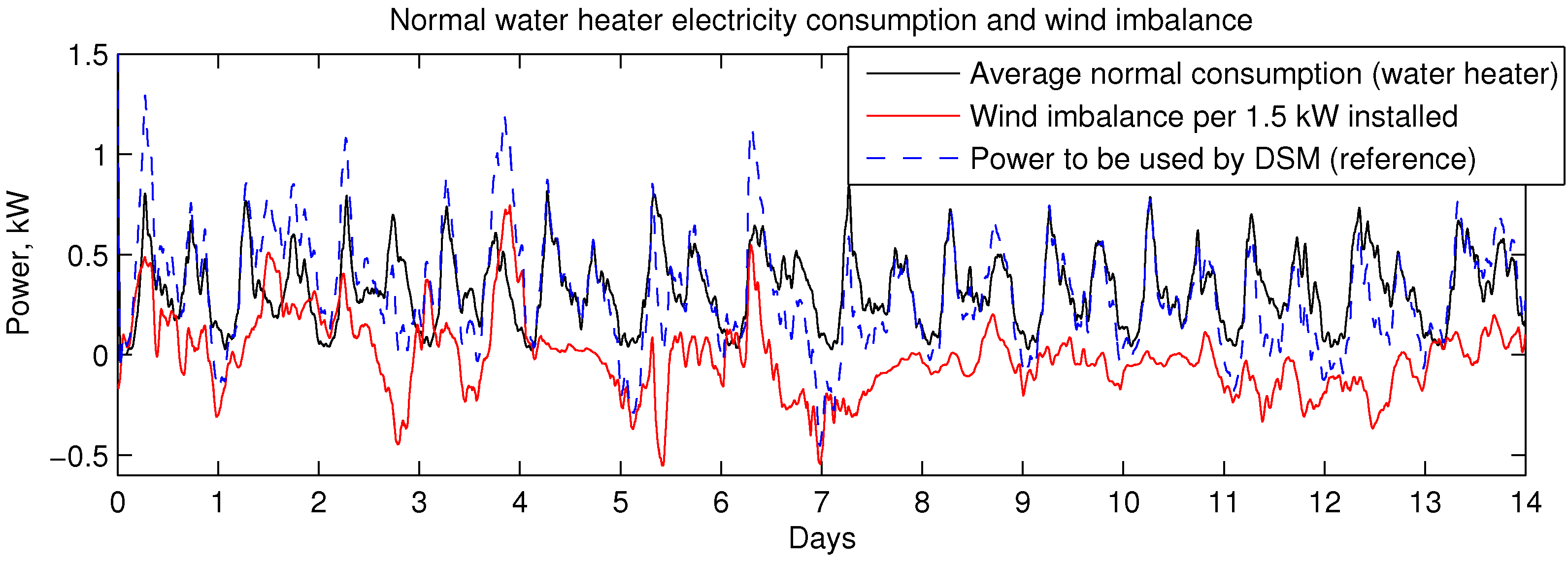
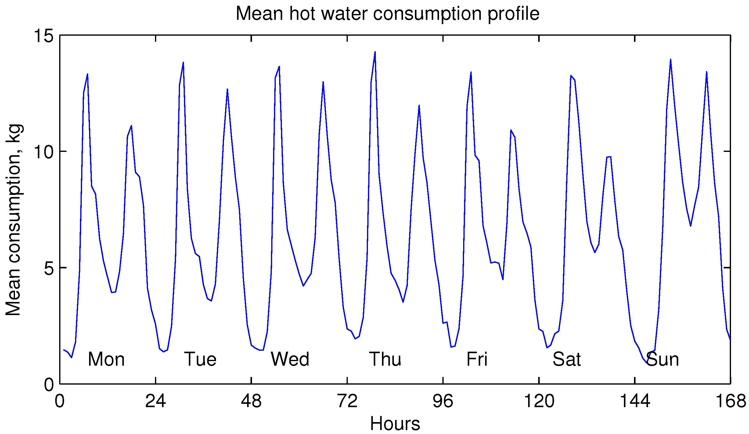
2.3. Wind Imbalance and Normal Consumption
2.4. Model Parameters and Assumptions
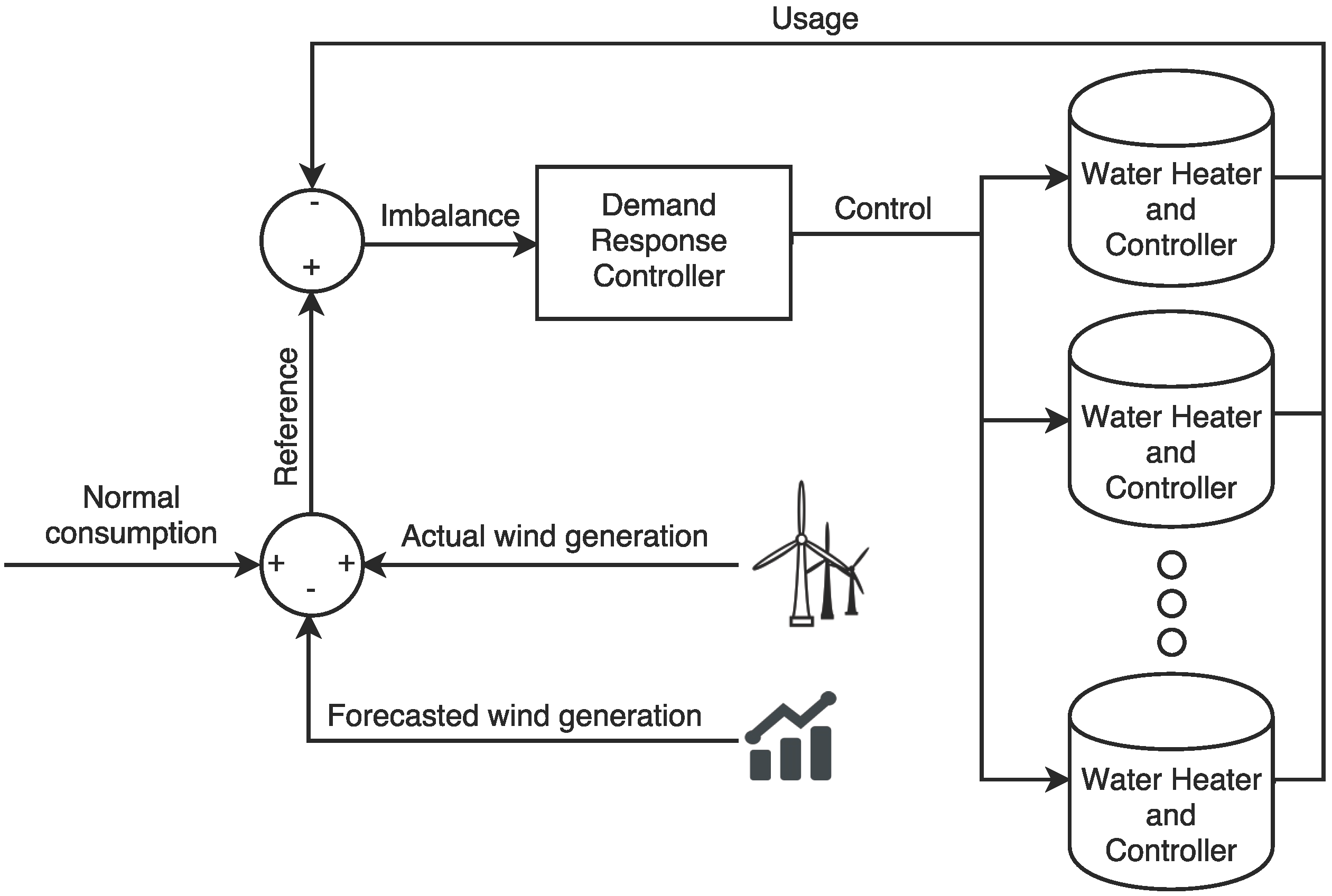
2.5. Proposed Demand Side Management System Overall Operation
3. Results and Discussion
- Mean power consumption is calculated by simply taking the arithmetic mean of the consumption profile from all dwellings.
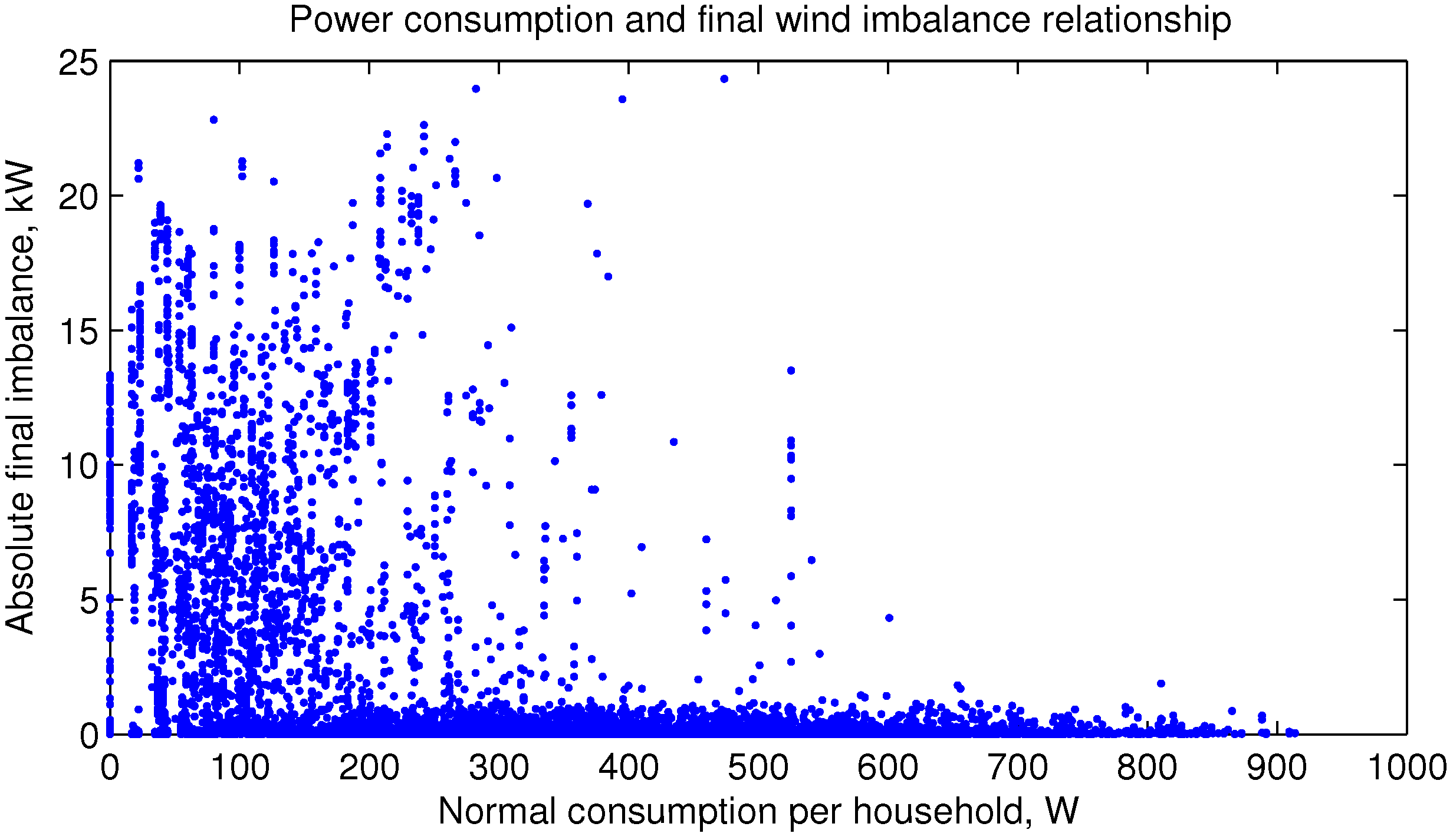
- Mean absolute final imbalance is the arithmetic average of final absolute imbalance values. Figures are scaled to be per household per 1.5 kW of installed wind power.
- Mean losses: arithmetic average of thermal losses per hot water heater.
- Mean temperature: arithmetic average of water temperature inside tanks.
- Shortage: average percentage of time the demanded water temperature was not supplied.
- Participation: the average percentage of time that each water heater was participating in DSM. The only time they are not participating is when there is expected high future consumption of hot water; thus, the temperature was expected to drop below critical, so the controller disconnects the particular water heater from DSM (therefore, increasing/maintaining user comfort).
3.1. Limitations
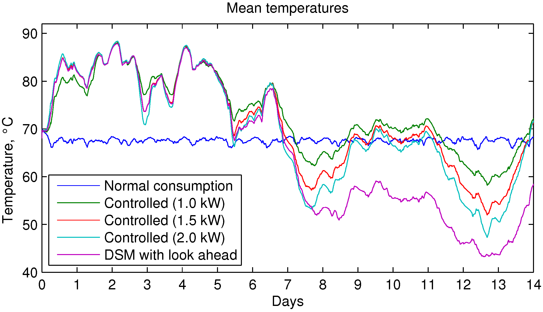
3.2. Temperatures
3.3. Losses
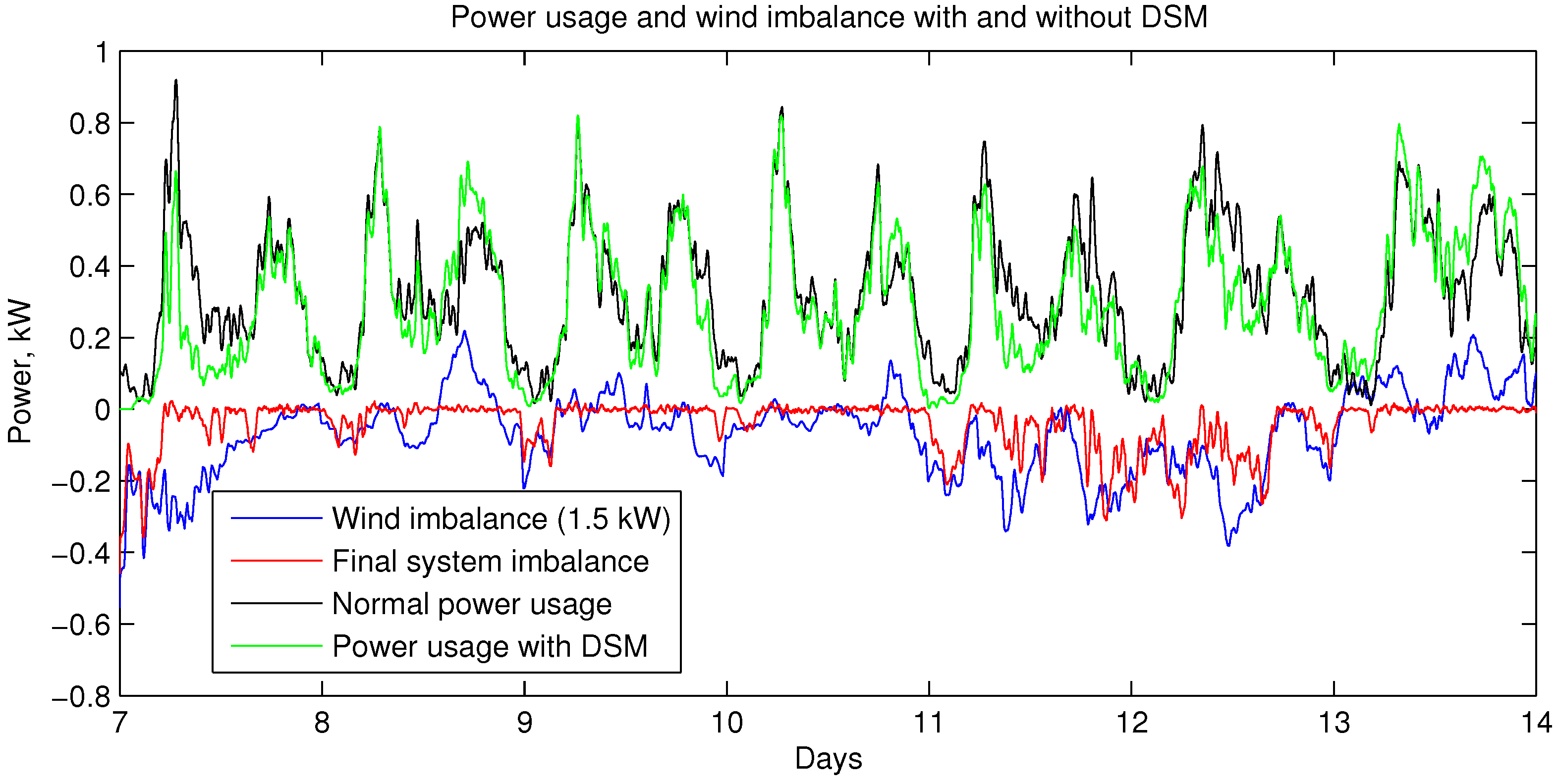
3.4. Energy Balance
4. Conclusions
Acknowledgments
Author Contributions
Conflicts of Interest
References
- Kundur, P. Power System Stability and Control; McGraw-Hill: New York, NY, USA, 1994. [Google Scholar]
- Baranauskas, A.; Gelažanskas, L.; Ažubalis, M.; Gamage, K. Control strategy for balancing wind power using hydro power and flow batteries. In Proceedings of the 2014 IEEE International Energy Conference (ENERGYCON), Cavtat, Croatia, 13–16 May 2014; pp. 352–357.
- Gelažanskas, L.; Gamage, K.A. Demand side management in smart grid: A review and proposals for future direction. Sustain. Cities Soc. 2014, 11, 22–30. [Google Scholar] [CrossRef]
- Lund, P.D.; Lindgren, J.; Mikkola, J.; Salpakari, J. Review of energy system flexibility measures to enable high levels of variable renewable electricity. Renew. Sustain. Energy Rev. 2015, 45, 785–807. [Google Scholar] [CrossRef]
- Pina, A.; Silva, C.; Ferrao, P. The impact of demand side management strategies in the penetration of renewable electricity. Energy 2012, 41, 128–137. [Google Scholar] [CrossRef]
- Doherty, R.; O’Malley, M. A new approach to quantify reserve demand in systems with significant installed wind capacity. IEEE Trans. Power Syst. 2005, 20, 587–595. [Google Scholar] [CrossRef]
- Wang, J.; Botterud, A.; Bessa, R.; Keko, H.; Carvalho, L.; Issicaba, D.; Sumaili, J.; Miranda, V. Wind power forecasting uncertainty and unit commitment. Appl. Energy 2011, 88, 4014–4023. [Google Scholar] [CrossRef]
- Finn, P.; Fitzpatrick, C.; Connolly, D.; Leahy, M.; Relihan, L. Facilitation of renewable electricity using price based appliance control in Ireland’s electricity market. Energy 2011, 36, 2952–2960. [Google Scholar] [CrossRef]
- Black, M.; Strbac, G. Value of Bulk Energy Storage for Managing Wind Power Fluctuations. IEEE Trans. Energy Convers. 2007, 22, 197–205. [Google Scholar] [CrossRef]
- Matos, M.; Bessa, R. Setting the Operating Reserve Using Probabilistic Wind Power Forecasts. IEEE Trans. Power Syst. 2011, 26, 594–603. [Google Scholar] [CrossRef]
- Gelažanskas, L.; Baranauskas, A.; Gamage, K.A.; Ažubalis, M. Hybrid wind power balance control strategy using thermal power, hydro power and flow batteries. Int. J. Electr. Power Energy Syst. 2016, 74, 310–321. [Google Scholar] [CrossRef]
- Divya, K.; Østergaard, J. Battery energy storage technology for power systems—An overview. Electr. Power Syst. Res. 2009, 79, 511–520. [Google Scholar] [CrossRef]
- Chen, H.; Cong, T.N.; Yang, W.; Tan, C.; Li, Y.; Ding, Y. Progress in electrical energy storage system: A critical review. Prog. Nat. Sci. 2009, 19, 291–312. [Google Scholar] [CrossRef]
- Denholm, P.; Sioshansi, R. The value of compressed air energy storage with wind in transmission-constrained electric power systems. Energy Policy 2009, 37, 3149–3158. [Google Scholar] [CrossRef]
- Hepbasli, A.; Kalinci, Y. A review of heat pump water heating systems. Renew. Sustain. Energy Rev. 2009, 13, 1211–1229. [Google Scholar] [CrossRef]
- Newborough, M.; Augood, P. Demand-side management opportunities for the UK domestic sector. IEE Proc. Gener. Transm. Distrib. 1999, 146, 283–293. [Google Scholar] [CrossRef]
- Armstrong, P.; Ager, D.; Thompson, I.; McCulloch, M. Improving the energy storage capability of hot water tanks through wall material specification. Energy 2014, 78, 128–140. [Google Scholar] [CrossRef]
- Paull, L.; Li, H.; Chang, L. A novel domestic electric water heater model for a multi-objective demand side management program. Electr. Power Syst. Res. 2010, 80, 1446–1451. [Google Scholar] [CrossRef]
- Ericson, T. Direct load control of residential water heaters. Energy Policy 2009, 37, 3502–3512. [Google Scholar] [CrossRef]
- Vanthournout, K.; D’hulst, R.; Geysen, D.; Jacobs, G. A Smart Domestic Hot Water Buffer. IEEE Trans. Smart Grid 2012, 3, 2121–2127. [Google Scholar] [CrossRef]
- Du, P.; Lu, N. Appliance Commitment for Household Load Scheduling. IEEE Trans. Smart Grid 2011, 2, 411–419. [Google Scholar] [CrossRef]
- Atikol, U. A simple peak shifting DSM (demand-side management) strategy for residential water heaters. Energy 2013, 62, 435–440. [Google Scholar] [CrossRef]
- Kepplinger, P.; Huber, G.; Petrasch, J. Autonomous optimal control for demand side management with resistive domestic hot water heaters using linear optimization. Energy Build. 2015, 100, 50–55. [Google Scholar] [CrossRef]
- Kondoh, J.; Lu, N.; Hammerstrom, D. An evaluation of the water heater load potential for providing regulation service. In Proceedings of the 2011 IEEE Power and Energy Society General Meeting, San Diego, CA, USA, 24–29 July 2011; pp. 1–8.
- Sedeh, M.M.; Khodadadi, J. Energy efficiency improvement and fuel savings in water heaters using baffles. Appl. Energy 2013, 102, 520–533. [Google Scholar] [CrossRef]
- Fitzgerald, N.; Foley, A.M.; McKeogh, E. Integrating wind power using intelligent electric water heating. Energy 2012, 48, 135–143. [Google Scholar] [CrossRef]
- Lu, N. An Evaluation of the HVAC Load Potential for Providing Load Balancing Service. IEEE Trans. Smart Grid 2012, 3, 1263–1270. [Google Scholar] [CrossRef]
- Nehrir, M.; Jia, R.; Pierre, D.; Hammerstrom, D. Power Management of Aggregate Electric Water Heater Loads by Voltage Control. In Proceedings of the 2007 IEEE Power Engineering Society General Meeting, Tampa, FL, USA, 24–28 June 2007; pp. 1–6.
- Measurement of Domestic Hot Water Consumption in Dwellings; Technical Report; Energy Saving Trust: London, UK, 2008.
- Celador, A.C.; Odriozola, M.; Sala, J. Implications of the modelling of stratified hot water storage tanks in the simulation of CHP plants. Energy Convers. Manag. 2011, 52, 3018–3026. [Google Scholar] [CrossRef]
- Gelažanskas, L.; Gamage, K. Forecasting hot water consumption in dwellings using artificial neural networks. In Proceedings of the 2015 IEEE 5th International Conference on Power Engineering, Energy and Electrical Drives (POWERENG), Riga, Latvia, 11–13 May 2015; pp. 410–415.
- Gelažanskas, L.; Gamage, K.A.A. Forecasting Hot Water Consumption in Residential Houses. Energies 2015, 8, 12702–12717. [Google Scholar] [CrossRef]
- Gelažanskas, L.; Gamage, K.A. Wind Generation; Data catalogue, Lancaster University Library: Lancaster, UK, 2015. [Google Scholar]


| Measure | Wind Generation | Hot Water Consumption |
|---|---|---|
| Forecast (per 1.5 kW) | Forecast (kg) | |
| Mean | 0.557 kW | 6.145 kg |
| Standard deviation | 0.374 kW | 9.269 kg |
| Mean error | −0.012 kW | 0.042 kg |
| Standard deviation of error | 0.137 kW | 1.541 kg |
| Mean absolute error | 0.099 kW | 0.870 kg |
| Root mean square error | 0.137 kW | 1.548 kg |
| Normalised mean absolute error [32] | 0.264 | 0.108 |
| Normalised root mean square error [32] | 0.368 | 0.192 |
| Regression value R | 0.938 | 0.981 |
| Case | Mean Power | Mean Absolute | Mean | Mean | Shortage | Participation, |
|---|---|---|---|---|---|---|
| Consumption (W) | Final Imbalance (W) | Losses (W) | Temperature (C) | (% of Time) | % | |
| #1 (N/A) | 325.7 | 144.3 | 49.4 | 67.5 | 0.11 | (N/A) |
| #2 (1.0 kW) | 309.4 | 26.6 | 54.4 | 73.1 | 1.19 | 100.0 |
| #2 (1.5 kW) | 298.7 | 47.1 | 52.6 | 71.4 | 1.95 | 100.0 |
| #2 (2.0 kW) | 290.0 | 72.3 | 51.2 | 70.0 | 2.74 | 100.0 |
| #3 (1.5 kW) | 313.9 | 52.1 | 46.9 | 65.9 | 0.30 | 94.0 |
© 2016 by the authors; licensee MDPI, Basel, Switzerland. This article is an open access article distributed under the terms and conditions of the Creative Commons by Attribution (CC-BY) license (http://creativecommons.org/licenses/by/4.0/).
Share and Cite
Gelažanskas, L.; Gamage, K.A.A. Distributed Energy Storage Using Residential Hot Water Heaters. Energies 2016, 9, 127. https://doi.org/10.3390/en9030127
Gelažanskas L, Gamage KAA. Distributed Energy Storage Using Residential Hot Water Heaters. Energies. 2016; 9(3):127. https://doi.org/10.3390/en9030127
Chicago/Turabian StyleGelažanskas, Linas, and Kelum A. A. Gamage. 2016. "Distributed Energy Storage Using Residential Hot Water Heaters" Energies 9, no. 3: 127. https://doi.org/10.3390/en9030127
APA StyleGelažanskas, L., & Gamage, K. A. A. (2016). Distributed Energy Storage Using Residential Hot Water Heaters. Energies, 9(3), 127. https://doi.org/10.3390/en9030127