
On Variable Reverse Power Flow-Part I: Active-Reactive Optimal Power Flow with Reactive Power of Wind Stations


Abstract
:
1. Introduction
- Introducing the reactive power capability of WSs in the optimization model of the active-reactive optimal power flow (A-R-OPF) and highlighting the benefits/impacts under different limits on PFs.
- Investigating the impacts of different agreements and variable reverse power flow on the operation of an ADN under different demand scenarios.
- Derivation of the function of reactive energy losses in the grid with an equivalent-π circuit and comparing its value with active energy losses.
- Balancing the energy curtailment of wind generation, active/reactive energy losses in the grid and active/reactive energy import/export by a meter-based method.
2. Problem Statement and Modeling Procedure
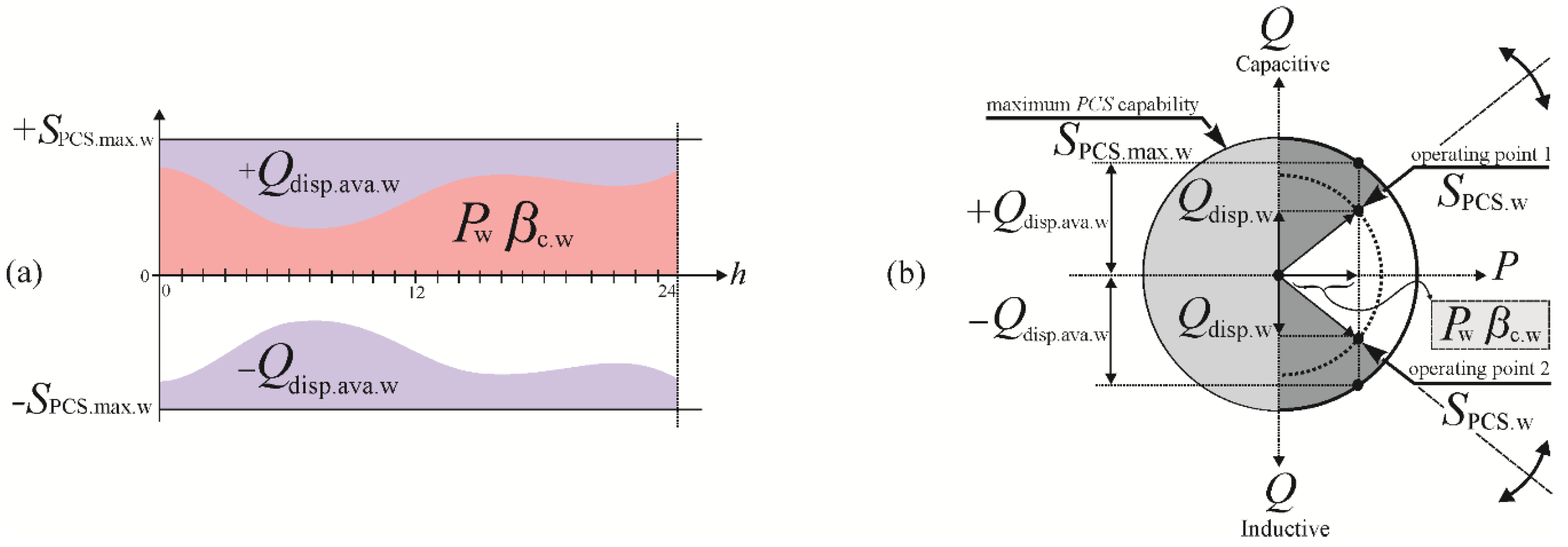
2.1. Wind Station
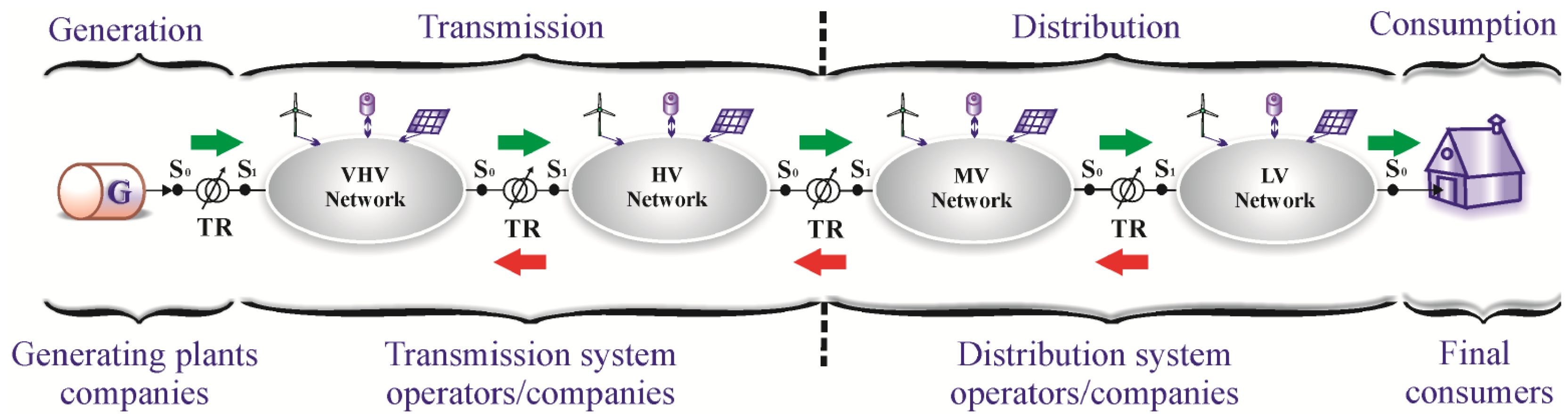
2.2. Substation Transformer
- ■
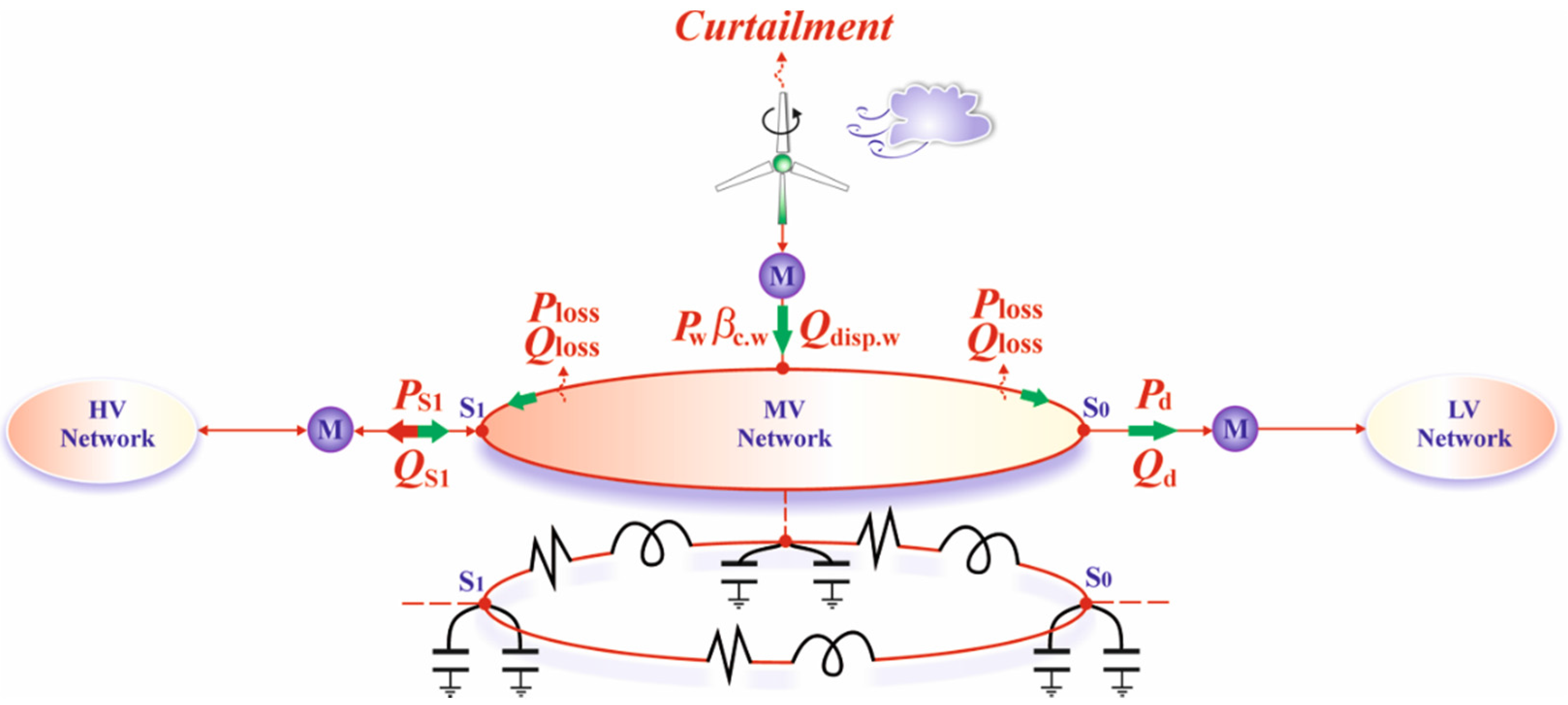
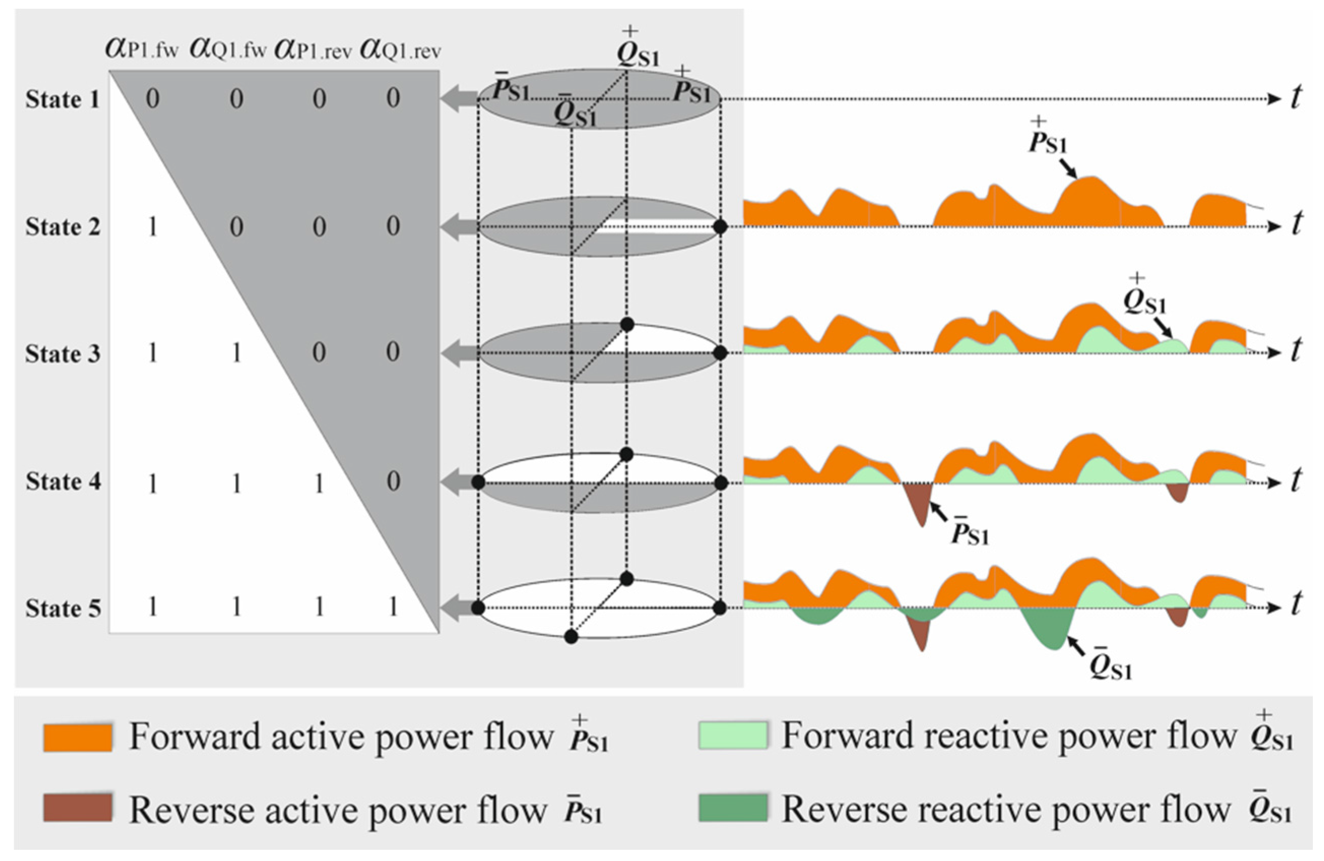
- State 1: This case represents an isolated power system where no active-reactive power is allowed to exchange between the upstream and downstream network at bus S1. In this case, renewable/conventional generating units and/or BSSs should be able to satisfy the active-reactive demand and losses inside the downstream network.
- ■
- State 2: Only active power is allowed to be imported (purchased) from the upstream network to satisfy the demand and losses in the downstream network. In this case, reactive power should be generated locally by suitable means to satisfy the reactive demand and losses in the downstream network.
- ■
- State 3: This case can be considered as the conventional state where powers are purchased from the network under a high voltage level. The purchased power must satisfy the active/reactive demand and losses in the network under a low voltage level. Note that in all states 1–3 renewable/conventional generating units and/or BSSs can be integrated in the downstream network, but no reverse active-reactive power is allowed to be sold to the upstream network.
- ■
- State 4: Active/reactive power is allowed to be purchased from the upstream network to satisfy all or part of the active/reactive demand and losses in the downstream network, but only reverse active power is allowed to be sold to the upstream network. In comparison to the states 1–3, additional agreements between the two sides should be declared for allowing bidirectional active power flows at bus S1.
- ■
- State 5: Both active and reactive powers are allowed to exchange between the upstream and downstream network. Here, more agreements are required before allowing bidirectional active-reactive power flows at bus S1.
2.3. Demand
3. Active-Reactive Optimal Power Flow with Reactive Power of Wind Stations
3.1. Objective Function
3.2. Equality Equations
3.3. Inequality Equations
3.4. Operating Conditions
- ▪
- ▪
- The system operator aims to maximize the benefits from wind power and meanwhile to minimize the costs of both active and reactive energy losses [23].
- ▪
- ▪
- The imported/exported reactive energy and reactive energy losses in the MV network are calculated by a given price model, i.e., the fixed (12 $/Mvarh) tariff price [16].
- ▪
3.5. Questions
- (1)
- What are the benefits/impacts of the “extended A-R-OPF model” for a real case power network?
- (2)
- What are the benefits/impacts of “varying PFs” of WSs in days with different levels of wind power generation?
- (3)
- How do the revenues/costs change with “variable reverse power flow” and “demand level” in an electricity market?
- (4)
- What are the relationships between the “location” of WSs, “variable reverse power flow” and “feeder congestion”?
4. Conclusions
Acknowledgments
Author Contributions
Conflicts of Interest
Appendix 1
| Functions | |
| F | Value of the objective function. |
| F1 | Revenue from wind power generation. |
| F2 | Cost of active energy losses. |
| F3 | Cost of reactive energy losses. |
| F4 | Cost/revenue of active energy at slack bus. |
| F5 | Cost/revenue of reactive energy at slack bus. |
| Parameters | |
| B(i,j) | Imaginary part of the complex admittance matrix. |
| Bse(i,j) | Imaginary part of the complex admittance matrix (series). |
| Bsh(i,j) | Imaginary part of the complex admittance matrix (shunt). |
| Cpr.p(h) | Price for active energy in hour h. |
| Cpr.q(h) | Price for reactive energy in hour h. |
| G(i,j) | Real part of the complex admittance matrix. |
| N | Number of buses. |
| Pd(i,h) | Power demand (active power) at bus i in hour h. |
| PW(l) | Rated installed power of wind station (WS) l. |
| Pw(i,h) | Wind power generation (active power) of WS at bus i in hour h. |
| Qd(i,h) | Power demand (reactive power) at bus i in hour h. |
| Sl.max(i,j) | Upper limit of apparent power for feeder located between bus i and j. |
| SS1.max | Upper limit of apparent power at slack bus. |
| SPCS.max.w(l) | Upper limit of apparent power of WS l. |
| Tfinal | Time horizon. |
| Vmin/Vmax(i) | Lower/upper limit of voltage amplitude at bus i. |
| State Variables | |
| Ploss/Qloss(h) | Active/reactive power losses in hour h. |
| PS1/QS1(1,h) | Active/reactive power produced/absorbed at slack bus in hour h. |
| S(i,j,h) | Apparent power flow from bus i to bus j in hour h. |
| SPCS.w(l,h) | Apparent power of WS l in hour h. |
| Qdis.ava.w(l,h) | Available reactive power of WS l in hour h. |
| Ve/Vf(i,h) | Real/imaginary part of the complex voltage at bus i in hour h. |
| V(i,h) | Voltage amplitude at bus i in hour h. |
| Control/Decision Variables | |
| Qdisp.w(l,h) | Reactive power dispatch of a WS l in hour h. |
| βc.w(l,h) | Curtailment factor of wind power at WS l during hour h. |
| PFmin.w(l) | Lower power factor of WS l. |
| PFmax.w(l) | Upper power factor of WS l. |
| αP1.fw | Forward-limit on active power at bus S1. |
| αQ1.fw | Forward-limit on reactive power at bus S1. |
| αP1.rev | Reverse-limit on active power at bus S1. |
| αQ1.rev | Reverse-limit on reactive power at bus S1. |
Appendix 2

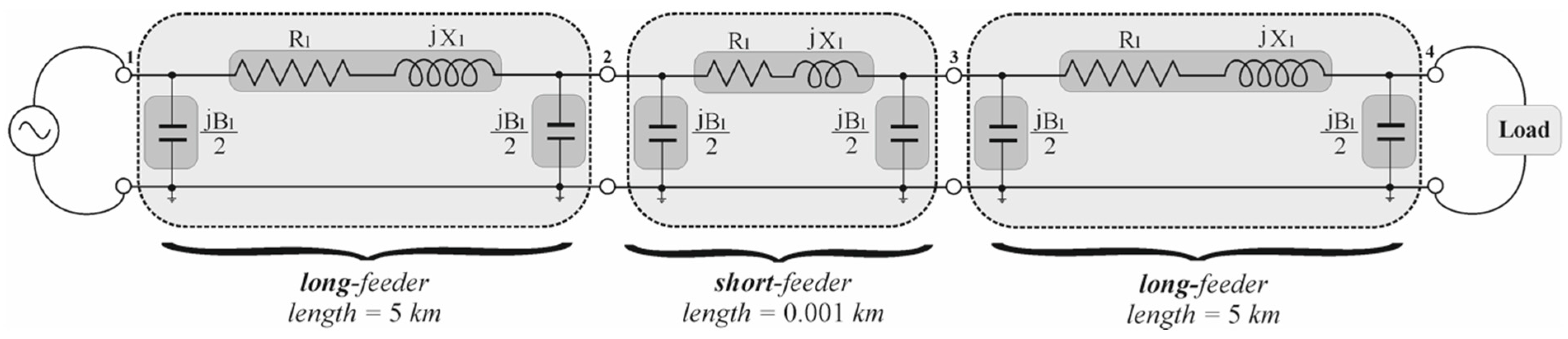
| No. Line | From Bus | To Bus | Line Type | Length (km) | Rl (ohm/km) | Xl (ohm/km) | Bl (μs/km) | Ampacity (MVA) |
|---|---|---|---|---|---|---|---|---|
| 1 | 1 | 2 | L1 | 5 | 0.169111 | 0.418206 | 3.954 | 20 |
| 2 | 2 | 3 | L1 | 0.001 | 0.169111 | 0.418206 | 3.954 | 20 |
| 3 | 3 | 4 | L1 | 5 | 0.169111 | 0.418206 | 3.954 | 20 |
| Pd (MW) | Qd (Mvar) | Ploss (MW) | Qloss (Mvar) | PS1 (MW) | QS1 (Mvar) |
|---|---|---|---|---|---|
| 10 | 6.2 | 0.33 | 0.77 | 10.33 | 6.97 |
| S(1,2) (MVA) | S(2,3) (MVA) | S(3,4) (MVA) |
|---|---|---|
| 12.461 | 12.112 | 12.110 |
References
- Schweppe, F.C.; Caramanis, M.C.; Tabors, R.D.; Bohn, R.E. Spot Pricing of Electricity; Kluwer: Boston, MA, USA, 1988. [Google Scholar]
- Gabash, A. Flexible Optimal Operations of Energy Supply Networks: With Renewable Energy Generation and Battery Storage; Südwestdeutscher Verlag: Saarbrücken, Germany, 2014. [Google Scholar]
- Kargarian, A.; Raoofat, M.; Mohammadi, M. Reactive power market management considering voltage control area reserve and system security. Appl. Energy 2011, 88, 3832–3840. [Google Scholar] [CrossRef]
- Kargarian, A.; Raoofat, M. Stochastic reactive power market with volatility of wind power considering voltage security. Energy 2011, 36, 2565–2571. [Google Scholar] [CrossRef]
- Khorramdel, B.; Raoofat, M. Optimal stochastic reactive power scheduling in a microgrid considering voltage droop scheme of DGs and uncertainty of wind farms. Energy 2012, 45, 994–1006. [Google Scholar] [CrossRef]
- Divya, K.C.; Nagendra Rao, P.S. Models for wind turbine generating systems and their application in load flow studies. Electr. Power Syst. Res. 2006, 76, 844–856. [Google Scholar] [CrossRef]
- Samimi, A.; Kazemi, A.; Siano, P. Economic-environmental active and reactive power scheduling of modern distribution systems in presence of wind generations: A distribution market-based approach. Energy Convers. Manag. 2015, 106, 495–509. [Google Scholar] [CrossRef]
- Aly, M.M.; Abdel-Akher, M.; Ziadi, Z.; Senjyu, T. Assessment of reactive power contribution of photovoltaic energy systems on voltage profile and stability of distribution systems. Electr. Power Energy Syst. 2014, 61, 665–672. [Google Scholar] [CrossRef]
- Kargarian, A.; Raoofat, M.; Mohammadi, M. Probabilistic reactive power procurement in hybrid electricity markets with uncertain loads. Electr. Power Syst. Res. 2012, 82, 68–80. [Google Scholar] [CrossRef]
- Haghighat, H.; Kennedy, S.W. A bilevel approach to operational decision making of a distribution company in competitive environments. IEEE Trans. Power Syst. 2012, 27, 1797–1807. [Google Scholar] [CrossRef]
- Burke, D.J.; O’Malley, M.J. Maximizing firm wind connection to security constrained transmission networks. IEEE Trans. Power Syst. 2010, 25, 749–759. [Google Scholar] [CrossRef]
- Burke, D.J.; O’Malley, M.J. A study of optimal nonfirm wind capacity connection to congested transmission systems. IEEE Trans. Sustain. Energy 2011, 2, 167–176. [Google Scholar] [CrossRef]
- Burke, D.J.; O’Malley, M.J. Factors influencing wind energy curtailment. IEEE Trans. Sustain. Energy 2011, 2, 185–193. [Google Scholar] [CrossRef]
- Gabash, A.; Xie, D.; Li, P. Analysis of influence factors on rejected active power from active distribution networks. In Proceedings of the IEEE Power and Energy Student Summit (PESS), Ilmenau, Germany, 19–20 January 2012; pp. 25–29.
- Gabash, A.; Li, P. Active-Reactive optimal power flow in distribution networks with embedded generation and battery storage. IEEE Trans. Power Syst. 2012, 27, 2026–2035. [Google Scholar] [CrossRef]
- Gabash, A.; Li, P. Flexible optimal operation of battery storage systems for energy supply networks. IEEE Trans. Power Syst. 2013, 28, 2788–2797. [Google Scholar] [CrossRef]
- Tonkoski, R.; Lopes, L.A.C.; El-Fouly, T.H.M. Coordinated active power curtailment of grid connected PV inverters for overvoltage prevention. IEEE Trans. Sustain. Energy 2011, 2, 139–147. [Google Scholar] [CrossRef]
- Tonkoski, R.; Turcotte, D.; EL-Fouly, T.H.M. Impact of high PV penetration on voltage profiles in residential neighborhoods. IEEE Trans. Sustain. Energy 2012, 3, 518–527. [Google Scholar] [CrossRef]
- Gabash, A.; Li, P. Active-Reactive optimal power flow for low-voltage networks with photovoltaic distributed generation. In Proceedings of the 2012 IEEE International Energy Conference and Exhibition (ENERGYCON), Florence, Italy, 9–12 September 2012; pp. 381–386.
- Oliveira, P.M.D.; Jesus, P.M.; Castronuovo, E.D.; Leao, M.T. Reactive power response of wind generators under an incremental network-loss allocation approach. IEEE Trans. Energy Convers. 2008, 23, 612–621. [Google Scholar]
- Zou, K.; Agalgaonkar, A.P.; Muttaqi, K.M.; Perera, S. Distribution system planning with incorporating DG reactive capability and system uncertainties. IEEE Trans. Sustain. Energy 2012, 3, 112–123. [Google Scholar] [CrossRef]
- Ullah, N.R.; Bhattacharya, K.; Thiringer, T. Wind farms as reactive power ancillary service providers—technical and economic issues. IEEE Trans. Energy Convers. 2009, 24, 661–672. [Google Scholar] [CrossRef]
- Algarni, A.A.S.; Bhattacharya, K. Disco operation considering DG units and their goodness factors. IEEE Trans. Power Syst. 2009, 24, 1831–1840. [Google Scholar] [CrossRef]
- López-Lezama, J.M.; Padilha-Feltrin, A.; Contreras, J.; Muñoz, J.I. Optimal contract pricing of distributed generation in distribution networks. IEEE Trans. Power Syst. 2001, 26, 128–136. [Google Scholar] [CrossRef]
- Mabeea, W.E.; Mannionb, J.; Carpenterc, T. Comparing the feed-in tariff incentives for renewable electricity in Ontario and Germany. Energy Policy 2012, 40, 480–489. [Google Scholar] [CrossRef]
- Stevens, R.H. Power flow direction definitions for metering of bidirectional power. IEEE Trans. Power Appar. Syst. 1983, 9, 3018–3022. [Google Scholar] [CrossRef]
- Levi, V.; Kay, M.; Povey, I. Reverse power flow capability of tap-changers. In Proceedings of the 18th International Conference Exhibition Electricity Distribution, Turin, Italy, 6–9 June 2005; pp. 1–5.
- Cipcigan, L.M.; Taylor, P.C. Investigation of the reverse power flow requirements of high penetrations of small-scale embedded generation. IET Renew. Power Gener. 2007, 1, 160–166. [Google Scholar] [CrossRef]
- Gabash, A.; Alkal, M.E.; Li, P. Impact of allowed reverse active power flow on planning PVs and BSSs in distribution networks considering demand and EVs growth. In Proceedings of the IEEE Power and Energy Student Summit (PESS), Bielefeld, Germany, 23–25 January 2013; pp. 11–16.
- Gabash, A.; Li, P. Reverse active-reactive optimal power flow in ADNs: Technical and economical aspects. In Proceedings of the 2014 IEEE International Energy Conference (ENERGYCON), Cavtat, Croatia, 13–16 May 2014; pp. 1115–1120.
- Gabash, A.; Li, P. On the control of main substations between transmission and distribution systems. In Proceedings of the 2014 14th International Conference on Environment and Electrical Engineering (EEEIC), Krakow, Poland, 10–12 May 2014; pp. 280–285.
- Gabash, A.; Li, P. Variable reverse power flow-part I: A-R-OPF with reactive power of wind stations. In Proceedings of the 2015 IEEE 15th International Conference on Environment and Electrical Engineering (EEEIC), Rome, Italy, 10–13 June 2015; pp. 21–26.
- Gabash, A.; Li, P. Variable reverse power flow-part II: Electricity market model and results. In Proceedings of the 2015 IEEE 15th International Conference on Environment and Electrical Engineering (EEEIC), Rome, Italy, 10–13 June 2015; pp. 27–32.


© 2016 by the authors; licensee MDPI, Basel, Switzerland. This article is an open access article distributed under the terms and conditions of the Creative Commons by Attribution (CC-BY) license (http://creativecommons.org/licenses/by/4.0/).
Share and Cite
Gabash, A.; Li, P. On Variable Reverse Power Flow-Part I: Active-Reactive Optimal Power Flow with Reactive Power of Wind Stations. Energies 2016, 9, 121. https://doi.org/10.3390/en9030121
Gabash A, Li P. On Variable Reverse Power Flow-Part I: Active-Reactive Optimal Power Flow with Reactive Power of Wind Stations. Energies. 2016; 9(3):121. https://doi.org/10.3390/en9030121
Chicago/Turabian StyleGabash, Aouss, and Pu Li. 2016. "On Variable Reverse Power Flow-Part I: Active-Reactive Optimal Power Flow with Reactive Power of Wind Stations" Energies 9, no. 3: 121. https://doi.org/10.3390/en9030121
APA StyleGabash, A., & Li, P. (2016). On Variable Reverse Power Flow-Part I: Active-Reactive Optimal Power Flow with Reactive Power of Wind Stations. Energies, 9(3), 121. https://doi.org/10.3390/en9030121