Modeling and Experimental Validation of a Low-Cost Radiation Sensor Based on the Photovoltaic Effect for Building Applications

Abstract

The energy consumed to cool buildings is very elevated and solar gains represent a high percentage of these cooling loads. To minimize the thermal load it is necessary to control external shading systems. This control requires continuous measurement of solar radiation in different locations of the building. However, for such applications the use of conventional irradiance sensors increases the cost and reduces the profitability of the installation. This paper is focused on the development, modeling, and experimental validation of low cost irradiation sensors based on photovoltaic effect in order to reduce the costs of dynamic external shading devices and to improve the profitability of the system. With this proposal, firstly, small commercial photovoltaic cells have been adapted for use as an irradiation measurement device. Subsequently, quasi-stationary and continuous experimental measurements of these silicon cells, facing south and installed horizontally, have been carried out in Jaén (Spain) in 2009 and 2010. Finally, a nonlinear multiparameter function has been developed to evaluate the irradiance using the electric current generated by the cell, cell temperature, ambient temperature, and absolute humidity. A favorable agreement between the model predictions and experimental data has been observed with a coefficient of determination around 0.996 for all cells.

1. Introduction

The energy consumption required to satisfy the demand for building cooling is very elevated. Globally, the sector’s final energy consumption doubled between 1971 and 2013 [1].

In light of this increased energy demand, the most recent version of the energy performance of buildings directive [2] requires that all new buildings be “nearly zero-energy” by 2020 [3], making energy efficiency optimization at every level an essential component of the construction process. There has been considerable activity over the past few decades investigating the life cycle energy of buildings. To reduce the life cycle energy of buildings, the focus has been on reducing their operational energy through improved design or equipment efficiency [4,5,6].

There is considerable evidence to suggest that most of the design changes which reduce the operational energy of buildings impact the embodied energy of the building. Ramesh et al. [7] have presented a critical review of life cycle energy analyses of buildings resulting from 73 cases across 13 countries. In this study different structural configurations within the same building are analyzed, for both offices and residences. Results show that operating (80%–90%) and embodied (10%–20%) phases of energy use are significant contributors to a building’s life cycle energy demand. Sartori et al [8] have analyzed the life cycle energy of 60 buildings in nine different countries, taking into account the different climatological variables and their effects. Case studies on buildings built according to different design criteria, but holding all other conditions constant, showed that design of low-energy buildings induces both a net benefit in total life cycle energy demand and an increase in the embodied energy. This research concludes that operational energy remains the dominant parameter and, when attempting to reduce the life cycle energy of buildings, the change in embodied energy can be generally ignored [7,8].

Since operational energy is generally larger than embodied energy in life cycle energy analysis, it has been studied widely in the literature. Different passive and active technologies have been suggested to reduce this energy [9,10,11,12,13].

Datta [14] has presented a study on the thermal performance of the building using different window shading systems and TRNSYS software (Version 14.2, Solar Energy Laboratory, University of Wisconsin, Madison, WI, USA) to model the simulations. The study took place in four Italian cities and configurations were optimized in each based on local meterological conditions. In Milan it was found that optimum shading cut down on solar gains by 70% in summer and 40% in winter, which is desirable. This research suggests that half the demand for building cooling is due to solar gains, which in turn vary based on local meterological conditions, and therefore shading systems must be specifically adapted to each location [14].

It is increasingly common to find buildings with a large glass area, which implies an increase in heat load that must be supported by air conditioning systems [15]. Palmero-Marrero et al. [15] have presented a general study on the effect of louver shading devices applied to different façades of a building, at different latitudes. Heating and cooling energy consumption was quantified for various types of windows and degrees of shading at different locations throughout the building. Mexico City (Mexico), Cairo (Egypt), Lisbon (Portugal), Madrid (Spain), and London (UK) have been analyzed in this study. The results suggest that shading systems reduce energy consumption significantly, while simultaneously making the internal environment more comfortable. Energy savings were more significant for cities with elevated ambiente temperatures and solar radiation, particularly Madrid, Lisbon and Cairo. However, in cities with lesser cooling demands, such as London, overly effective shading systems are not apt, and may in fact increase energy consumption in winter when the buildings require more artificial heating. For these cases, automated dynamic shading systems are recommended.

There are different systems that are able to intercept direct radiation, such as overhangs, venetian blinds, external roller shades, etc., and their effects have been studied [15,16,17,18,19,20,21].

External shading systems are the most effective means of reducing cooling demands as they prevent solar radiation for heating the building [22,23,24].

Gratia et al. [22] have analyzed the influence of the position and the color of the blinds on the cooling consumption of an office building with a double skin façade. The simulations were performed in a medium-sized office building with climatic data from Uccle (Belgium). This research concludes that external solar protections are more effective than internal shading devices. The judicious choice of the location and the size of the blinds makes it possible to save up to 14.1% of the cooling consumption of the entire building on a sunny summer day.

Kim et al. [23] have verified the advantage of the external device in South Korea, various types of shading devices have been analyzed and compared with the experimental configuration proposed in terms of energy savings for heating and cooling by using simulations.

Their results suggest that in the cooling season, conventional blinds with declining slats save cooling energy by 10% and the external shading device is much more effective than any internal device since an internal device absorbs solar heat and radiates it to the interior.

Fenestration products that are fully shaded from the outside reduce solar heat gain by as much as 80% [25,26]. The influence of external solar shading devices on the energy requirements of a typical air-conditioned office building designed for Italian climates has been analyzed by Bellia et al. [26]. In this study, the annual energy demand required for heating, cooling and lighting has been calculated, as well as the influence of shading systems on cooling energy demand reduction as a function of the architectural design. The study concludes that annual energy savings depend on the building’s location, achieving the greatest reduction in energy consumption in warmer climates, 20% in Palermo as opposed to 8% in Milan, with a cooler climate [26].

The solar shading devices also allow a useful reduction in peaks for summer electric energy demand [27].

Solar shading systems reduce levels of natural light in a building and reduce yearly solar gains. Therefore, shadings affect the building energy use for lighting, heating and cooling, and also the occupants’ visual and thermal comfort [28,29].

Automated external shading systems are a fundamental element of the façade, and increase both the energy efficiency of the building as well as improve occupant confort [30]. An interesting way to decrease energy demands in buildings where domotics are integrated, is by controlling the different external shading devices using instantaneous radiation measurements as the control parameter [31]. Sensors for measuring solar radiation are necessary to control dynamic shading. These are placed on the roof, exterior façade, next to the windows, or inside windows surfaces to measure global solar radiation. Subsequently, shading control algorithms using the value of solar radiation to operate shading systems adjust the tilt angle of the venetian blinds [32,33], opening or closing of shutters and blinds [31,34,35,36]. Several studies of shading control algorithms based on solar radiation measurements have shown great potential for energy savings [20,30,32,37,38].

There has been previous research into dynamic fenestration technologies to determine their significance in relation to energy consumption and occupant comfort. Results show the potential of dynamic fenestration components, ranging from a decrease in cooling and lighting demand [20,39], reduced overall energy demand [40], and improved daylight utilization [41].

However, dynamic solar shading with its ability to reduce energy consumption and improve occupant comfort may not always be the optimal choice when economics (acquisition and maintenance) or subjective factors, such as aesthetics, are considered [30].

Some previous studies have analyzed the influence of costs on the profitability of this type of installation [42]. They emphasize the importance of reducing costs to increase the viability of these installations. However, few research investigations have been carried out to reduce the costs of this type of installation. Furthermore, reducing the costs of solar radiation sensors has rarely been considered as another way to reduce costs and increase the competitiveness of these installations [43].

Muñoz-García et al. [44] have developed a low-cost sensor that permits the measurement of irradiance inside the tree canopy. For these applications, it is necessary to take measurements at various heights and test points, requiring multiple sensors, thus increasing the cost of the experiment, and making conventional irradiance sensors unsuitable. Experiments were performed in Ademuz (Valencia, Spain). The observed difference between solar irradiation at high and low positions was 18.5% ± 2.58% at a 95% confidence interval. The objective of this work was to evaluate the effectiveness of a means to detect solar irradiation using a more cost-effective irradiance sensor with an acceptable error (±5%), adequate for applications where a relative evaluation of irradiance in a distributed area is of high importance.

Plesz et al. [45] have studied the working principle, design, and thermal characterization of a low cost solar irradiation sensor. The sensor is based on a photoelectric cell and thermal tests were performed in a climate chamber in the temperature range of −20–80 °C in increments of 10 °C. They conclude that the self-made solar cell’s thermal dependence was 0.26% °C⁻¹, revealing higher temperature dependence than in the case of an industrial reference cell.

Other research has aimed to develop low cost sensors that can be used in windows with efficiently-controlled dynamic glazing, which offer a high potential for controlling solar heat gain and minimizing heating, cooling and lighting loads. Dussault et al. [46] has presented two designs of a new type of low cost sensor for solar heat flux measurements in buildings. The black and white sensor (BWS) uses the difference in temperature between a white surface and a black surface to estimate the solar heat flux through building openings. The two designs of BWS have shown mean weighted relative errors under 4% over the sampling periods for the daily integrated solar energy measured.

The profitability of the automated dynamic solar shading system depends largely on the initial cost of installation. Reducing the cost of measurement systems likewise reduces the cost of installation and, thus, helps to make solar shading a better choice. Hence, the main objective of this paper is the development, modeling and experimental validation of low cost irradiation sensors in order to reduce the costs of dynamic external shading devices and to improve the profitability of the system. The most important factor when using photodetectors (solar cells) to estimate solar radiation is temperature dependence [47].

Firstly, to evaluate the influence that the temperature of the cell has on the response of the system, a temperature sensor has been added to a commercial photovoltaic cell. The calibration curve provided by the cell’s supplier is not useful in this case because it is made for a constant 20 °C temperature.

Secondly, the experimental setup and characteristics of the tests performed are described. The cell’s response has been measured and the results have been compared to values of irradiance and other weather conditions obtained from the website of the University of Jaén Research Group of Atmosphere Modeling and Solar Radiation (MATRAS) [48].

Finally, with these data, a procedure for recalibrating the system has been evaluated to use the cell as a radiation measurement device.

The results obtained are presented and discussed in terms of establishing the relationship between the temperature cell, intensity, and ambient conditions, and how it relates to solar radiation.

The main contributions of this paper are: the methodology developed to adapt solar cells for estimating solar radiation; the tests conducted to determine thermal dependence and adjust the model; and the procedure used to set a nonlinear multiparameter function which can determine the solar radiation of any of these cells with a coefficient of determination higher than 0.996 for all cases. Comparable expressions to estimate solar irradiation using photovoltaic sensors have not been previously found in the literature.

2. Background: The Use of Solar Cells for Irradiation Assessment

The solar radiation measurements are taken by instruments, like pyranometers, which measure the global incident solar radiation, usually on horizontal surfaces. Thermoelectric and photoelectric types are the most commonly used sensors to evaluate solar irradiation and mathematical models to describe commercial photovoltaic module have been proposed [49,50] Photoelectric sensors normally apply silicon solar cells and measure their short circuit current [51]. Such sensors are simple in construction [52] and the light intensity can be converted directly to an electrical signal. Devices based on silicon technology are frequently used for energy applications [53]. Some of these devices, like the Kipp and Zonen SP_LITE2 (Kipp & Zonen USA Inc., Bohemia, NY, USA), are commercially available for around 355 € (3 April 2015) [54], which is prohibitively expensive for the purposes of this study. Nevertheless, it is still possible to construct a precise device for measuring irradiance at a reduced price by using low-cost sensors based on the photovoltaic effect [44].

Small commercial photovoltaic cells have been used in this study. These cells are not very precise and are designed for applications which require an estimated value of solar radiation. The supplier has used a solar simulator to calibrate the original cells. This equipment allows us to establish a similar spectrum and radiation to that of natural sunlight, and to set a desired value. With these experimental devices it is possible to establish the air mass (m), which is the inverse cosine of the sun zenith angle θ_Z [55]. The original calibration curve provided by the supplier (Figure 1) is calculated only for m = 1.5 and a cell temperature of 20 °C. However, these values are not representative of the wide range of possible atmospheric conditions that occur in nature and, therefore, the curve cannot be used if one wants to have a precise measurement of solar radiation. The running of these sensors based on the photovoltaic effect is similar to that of a photodiode, such that the incident solar radiation, as well as the temperature, affects the element’s response. This same technology is currently being used for electricity generation in photovoltaic cells. It is known that when incident solar radiation has a high incidence angle on the cells, the efficiency is high, because of the low temperature of the cells, near to the calibration temperature of 20 °C. Nevertheless, when the beam component of the irradiance increases, the cell temperature rises while its efficiency decreases [56].

In addition, changes in external conditions (solar radiation, ambient temperature, and relative humidity) affect the temperature and in turn, temperature changes influence both the signal processing circuit and solar cell parameters [57] and, thus, reduce the accuracy of the irradiation measurement [58]. The most important factor is temperature dependence [47] and, therefore, the thermal effects must be considered when selecting and testing the components used for the device, due to outdoor use of the sensor. Proper calibration should take into account not only the response of the cell (electric current) but also its temperature for different values of incident radiation and atmospheric conditions. The purpose is to determine a function that is able to evaluate the irradiance using the temperature and intensity of the cell, as well as the relative humidity and ambient temperature as inputs.

The limited applicability of these original cells is what justifies its reduced price of 15 euros per cell. This reduced price has allowed us to adapt the cells and convert them into more accurate sensors that can be used for applications in the building sector, while maintaining low prices of around 40 euros per unit.

3. Materials and Methods

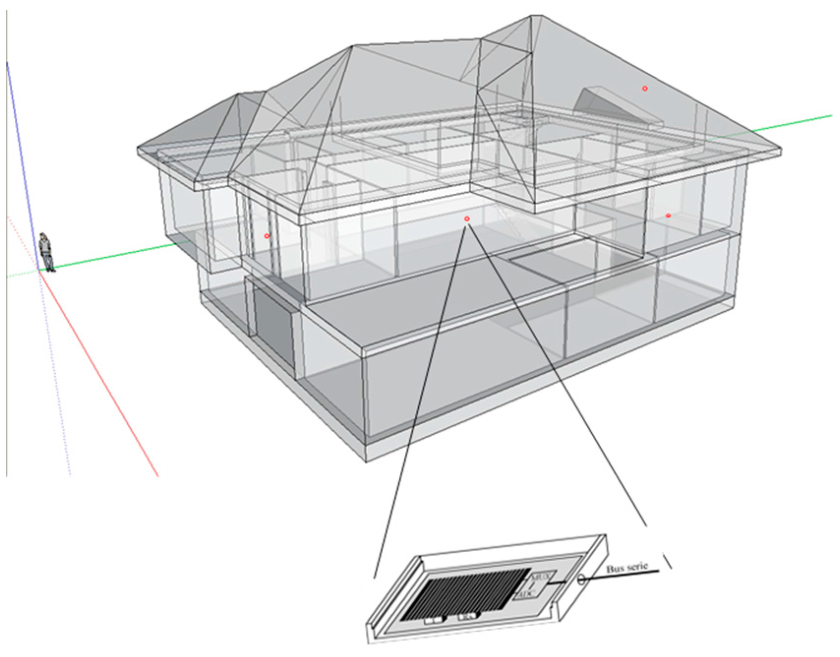
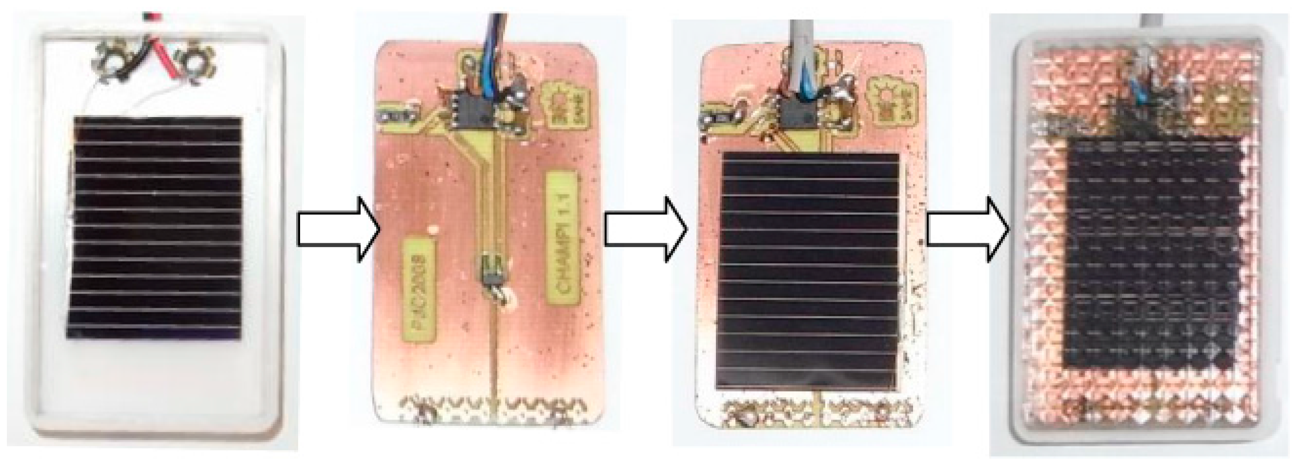
3.1. Devices

Given a building geometry, the control of passive systems, such as blinds and awnings, can be made by placing low-cost radiation sensors at different locations in the building as shown in Figure 2.

The measurement system that has been developed for a price of around 40 euros has two sensors, a radiation sensor and a temperature sensor, connected to an analog-to-digital converter (ADC) with four channels and eight bits [51].

To measure irradiance R (W/m²), small, high-efficiency single-crystal silicon cells with the dimensions 3.5 cm × 5.5 cm are used. This radiation sensor delivers an electric current I_p (mA) proportional to the incident solar radiation, with accuracy close to 275 μA/Wm⁻² (this changes depending on the device and has to be obtained during the calibration process).

Using a shunt resistor (R_s) of 1 Ω, the electric current is converted into voltage and introduced to the converter (ADC) with a sensitivity close to 0.275 mV/Wm⁻². This procedure is similar to that used in the case of industrial sensors where the solar cell´s short circuit is often ensured by a small resistance, and the voltage across this resistance is proportional to the intensity [59].

Afterwards, a device to measure the temperature of the cell T_p (°C) is added. This sensor is an integrated type and provides a voltage which is proportional to the temperature with a ratio of 10 mV/°C and a minimum value of 0.1 V for −40 °C. This device is attached to the radiation sensor with silicone, in order to reduce the thermal resistance (Figure 3).

Generated voltages by every sensor are digitized via two of the four available channels in the ADC. The ADC has a digital output (one-wire serial bus), which allows the connection of multiple measurement systems to a data-only transmission wire [60].

The voltage range at the converter ADC input goes from 0 V to 2.56 V, so the resolution obtained with the available eight bits is 10 mV/bit, that is, an accuracy close to 36 Wm⁻² for the radiation measurement and close to 1 °C for the temperature measurement. The software adapts voltage signals to intensity and temperature values, and saves this data in files. In total, 31 sensors have been adapted to monitor the solar radiation.

3.2. Testing Section

In order to determine a function that is capable of achieving a favorable agreement between the model predictions and experimental data, tests covering a complete range of atmospheric conditions are necessary. There are papers that have modeled the thermal dependence of this type of sensor performing laboratory tests [45], and other authors with similar objectives have carried out the tests in outdoor conditions [44]. In this case, the use of natural radiation was chosen, tests were carried out in outdoor conditions in order to model the influence of the transient thermal drift as realistically as possible.

Firstly, to use the solar cells as solar radiation sensors, the cells were preconditioned to sunlight and then calibrated over a period of two weeks. This step is mandatory for silicon solar cells. During the pre-conditioning period, the solar cells achieved their final electrical characteristics. This means that the electrical characteristics of the cell achieved a stable state after a decrease in their value in the initial weeks of exposure to sunlight with an average decrease of 5 mA in the real current compared with the original calibration curve. The cell calibration process was sufficient to ensure that a stable state had been reached [44].

Experiments were been performed over two years (2009 and 2010) in a building at the University of Jaén, located in Jaén (Spain), GPS coordinates 37°47′13.7″ N, 3°46′39.9″ W. They took place over the course of 48 days in 2009 and 49 days in 2010. The 31 solar cells, described above, were tested.

For the calibration, a large number of experimental measurements were taken with each cell using natural radiation during the period described above, with a horizontal position for the cells. In every test, the incident radiation value on horizontal surfaces R (W/m²) was checked against values from the website of the University of Jaén research group, MATRAS. MATRAS uses accurate devices located on the terrace roof of the same building where the tests were performed. Two types of tests were performed: quasi-stationary tests and continuous tests.

For the quasi-stationary tests, at various times of day and on different days, from sunrise to sunset, the electrical current generated by the cell and its temperature were measured for 10 min, time enough to ensure a negligible change in the incident solar radiation. However, a change in the temperature of the cell during the length of every test can be observed, a change which also affects the intensity of the resulting current. Therefore, the cell must be cooled down at the beginning of every new test measurement. The purpose of these tests has been to observe significant changes in variables along the heating process of the cell when the irradiance remains practically constant. This type of test allows us to determine the dynamic behavior of the cell, moreover, since the response of such sensors is very fast [61] and tests were carried out with small sampling times, the transient behavior of the cell has been registering with elevated detail.

For the continuous tests, however, electric current and temperature data of the cell were measured nonstop for complete day cycles in various weather conditions. Thus, a full range of temperatures and solar angles was measured. A multiparameter function was adjusted using the continuous test. The dataset was divided into two groups to develop the model. The first group, including two-thirds of the total data, was used for model development, whereas the remaining one-third was reserved for validation purposes. All test data are saved in PC files.

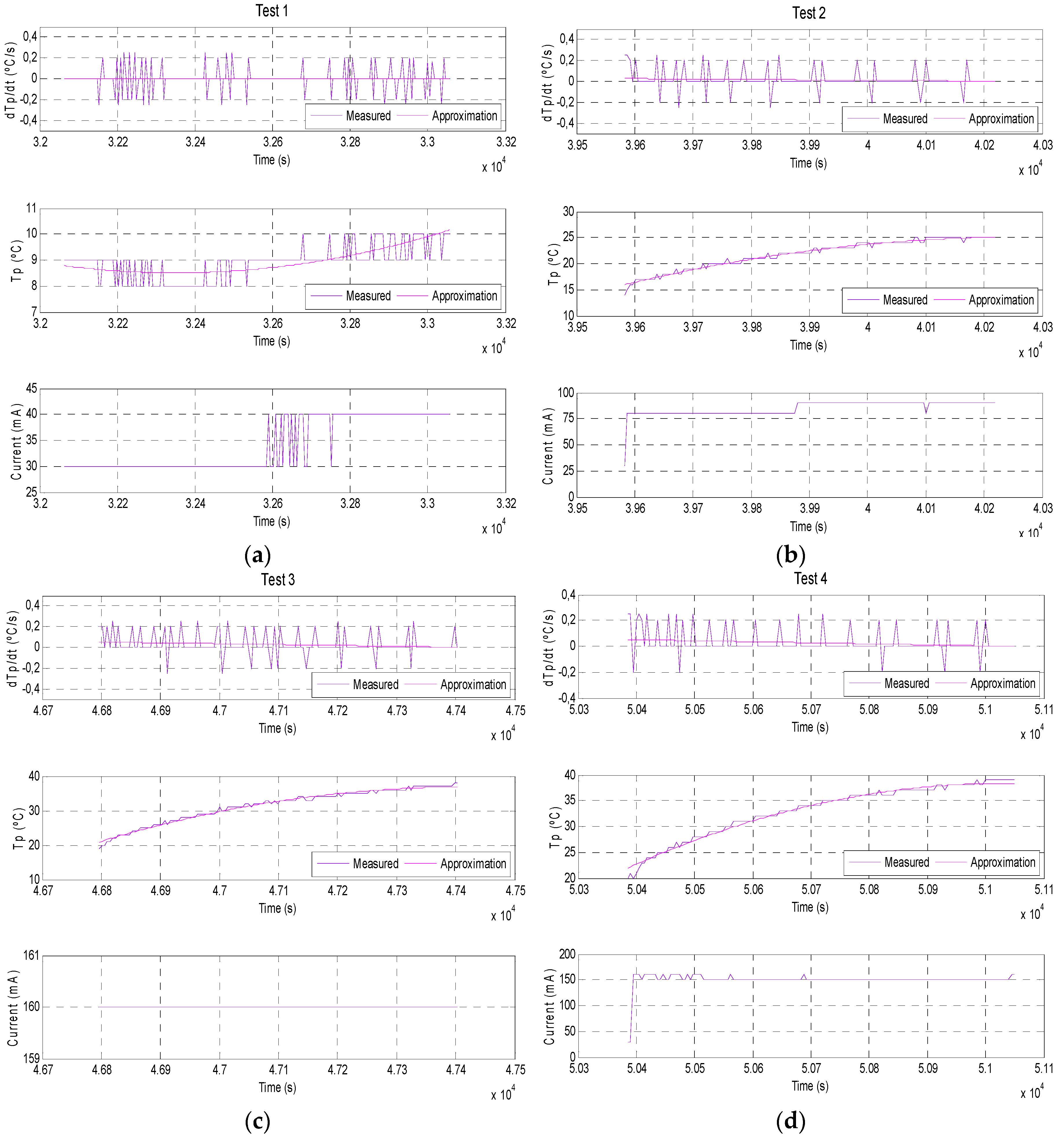
3.3. Thermal Model and Response Fitting

The temperature response is dynamic when the irradiance changes. Thus, several investigations have modeled the temperature of a photovoltaic (PV) module evaluating the energy inputs and outputs through radiation, convection, conduction, and power generated, via transient methods [62,63,64]. Other analyses have been conducted searching linear regressions from ambient data [65]. In [66] a formula is included in which solar irradiance is related to the electric current generated by a cell that can be used to determine solar radiation in applications like those presented in this paper. In [44] the authors have simplified this formula by not taking cell temperature into account, and it has been used to estimate solar radiation inside tree canopies using calibrated photodetectors with an acceptable error (±5%) adequate for their application. In the present study, the main contribution is the development of a methodology to improve the accuracy of the model by measuring the individual temperature of every particular cell, as well as the relative humidity and ambient temperature.

For the present study, a previous approach established the relationship between temperature cell, power generation and ambient conditions, searching a linear dependence between them [51]. A high accuracy model with thirteen variables was obtained, but there were discrepancies between the punctual (quasi-stationary) and continuous measurements, indicating that a linear relationship did not accurately model the physical variables.

In this work, to improve the fit between the model predictions and experimental data, the variables to be searched must follow the main terms associated to the energy balance (first law of thermodynamics) applied to the system. This establishes that the net heat Q transferred is equal to the sum of the internal energy U change and the amount of energy transferred from the system by work W [67]:

$${\displaystyle \sum }\frac{\mathrm{d}Q}{\mathrm{d}t}=\frac{\mathrm{d}U}{\mathrm{d}t}+\frac{\mathrm{d}W}{\mathrm{d}t}$$

(1)

The left term takes into account the irradiance input from the sun R (W/m²), as well as the heat loss from the system ΣdQ_L/dt (W) by convection, conduction, and radiation mechanisms. Models applied to PV systems consider all these terms, setting up the rate of temperature change as the sum of these contributions. Jones and Underwood [63] establish a detailed expression considering all the individual terms for a PV module, considering the module heat capacity, short wave radiation heat transfer, long wave radiation heat transfer, convection heat transfer, and electrical power generation, complementing previous studies. The main difference in this case is that a plastic covering appears at the top of the structure, creating a greenhouse effect similar to a thermal system.

The transmittance-absorptance product τα (dimensionless) of the plate and covering, altogether, must be considered, according to the associated model of a thermal system [55]. Thus, the input heat flow to the system comes from the sun, with global irradiance R (W/m²), proportionally affected by the cell surface S (m²), as well as the product τα. A detailed analysis of this last term [55] initially establishes a direct relationship with the angle of incidence of radiation θ (rad).

On the other hand, the rate of internal energy change considers the rate of the plate temperature change dT_p/dt and a net heat capacity C (J/kgK) of the materials of the device, such as the cell, the temperature sensor, and the conductive paste that connects both sub-systems. The net work transferred consists of the electrical power generated W (W), obtained as a result of multiplying the square of the current I_p (A) and the shunt resistance R_s (Ω).

The most complex term to be analyzed comes from the heat loss evaluation ${\dot{Q}}_L$ [68]. A detailed evaluation must consider the surrounding environment, with temperature T_a (K) and relative humidity H_r (%). Associated models consider the conduction-convection heat transfer mechanism throughout the global heat coefficient K (W/m²K), cell radiation emission losses, mainly depending on T_p⁴, or a sky model [69]. The radiations are exchanged between the grey surfaces and the cell box, and the small dimensions of the whole device further increase the loss analysis.

Considering all of the assumptions described above, the system can be characterized by a dynamic behavior using Equation (2):

$$\left(\mathsf{\tau }\mathsf{\alpha }\right)RS-{\displaystyle \sum }{\dot{Q}}_L=C\frac{\mathrm{d}{T}_p}{\mathrm{d}t}+I_p^2{R}_s$$

(2)

The reduced mass and geometry of the device, shown in Figure 1 and Figure 3, make it difficult to achieve an adequate approach directly applying the expression in Equation (2). It is, therefore, necessary to include some important notations regarding the terms of the model that will facilitate their implementation:

(a)

It is necessary calculate the temporal derivative of cell temperature. As the temperature can be measured at each moment, its derivative can be approached.

(b)

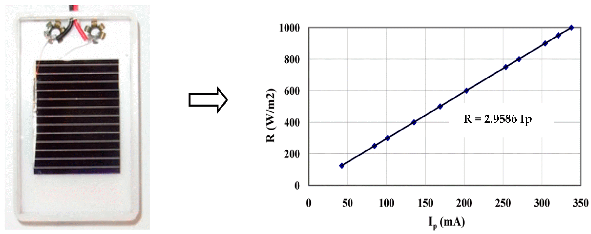
Electric current is provided by the cell through the shunt resistance.

(c)

Ambient conditions (temperature, humidity, irradiance) can be measured.

(d)

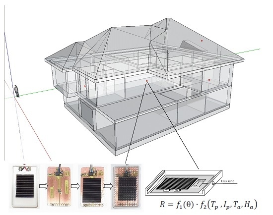
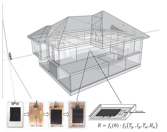
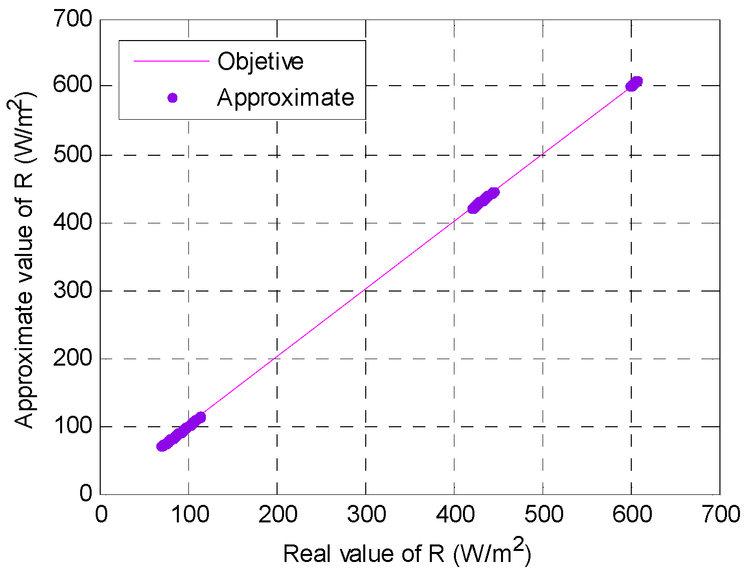
Finally, there exists a nonlinear relationship between irradiance R and the other variables by the transmittance-absorptance product.

Thus, a parametric approach of R following the logical disposition of the different terms in Equation (2) can be described as follows:

$$R=f_1\left(\mathsf{\theta }\right)·f_2\left(T_p,I_p,T_a,H_a\right)$$

(3)

Once these tests were finalized, radiation data R (W/m²) were obtained relative to the electric current generated by the cell I_p (mA) and its temperature T_p (°C). Meteorological parameters, such as ambient temperature T_a (°C) and relative humidity H_r (%), were also taken into account. Absolute humidity H_a (kg water/kg dry air) was deduced from these data [67].

Then, a multiparameter function is adjusted to evaluate the irradiance. As the response is nonlinear, it is necessary to turn to a least squares approximation using nonlinear techniques, such as those based on the Newton method [70]. To determine the suitability of the approximation function, the coefficient of determination r² has been used in order to establish the robustness of the characterization [71].

4. Results and Discussion

Table 1. Weather conditions for punctual measurements on 2 February 2010. GMT: Greenwich Mean Time.

Test No. (GMT)	1 (8 GMT)	2 (10 GMT)	3 (12 GMT)	4 (13 GMT)
R (W/m2)	100	432	605	602
Ta (°C)	3	8	11	12.5
Hr (%)	76	60	50	35

indicates the weather conditions for the measurements (MATRAS website [48]) taken on 2 February 2010 for various time zones with respect to Greenwich Mean Time (GMT).

Quasi-stationary measurements performed on 2 February 2010 of electric current and cell temperature in one test is showed in Figure 4. The legend denoted “measured” is the irradiance measured by an independent calibrated sensor and the legend denoted “approximation” (corrected signal) refers to the irradiance calculated using the developed model. The natural irradiance suffers very little changes since each test lasts 10 min. The rate of temperature change can also be observed, obtained by differentiating the cell temperature.

There exist significant changes to these variables during the heating process of the cell, although irradiance suffers very little change. This kind of test is ideal for determining the dynamic behavior of the cell. Some considerations can be drawn from the Figure 4.

The temperature cell data present plenty of ripple, due to the very small sampling time in the measurements (close to 3 s). Likewise, there are oscillations in the temporal response, due to the sensor itself. In any case, the temperature evolution during each experiment presents a polynomial trend.

Regarding the generated electric current, there is no ripple and the changes in the response occur only occasionally, in moments when certain oscillations occur as well. The ripple effect in temperature measurements appears as a consequence of the sensor itself, while in the other case, there is a non-desired effect caused by the limited resolution of the measurement system, which is not able to read variations inferior to 10 mA in the system response.

In any case, there are drift effects due to the fact that the conditions showed in Table 1 are not constant during the test and, although the changes are very slight, they do occur and are reflected in the response. The occasional appearance of clouds during the test leads to results which are non-comparable to the results given by the weather station since their results correspond with mean values of irradiance every 10 min. In addition, photovoltaic sensors have faster time responses than thermal sensors, 10 µs versus time constant in the order from 1–10 s [61,72].

The errors associated with the response time tend to be eliminated with integrated measurements [73]. Consequently, from these results it is deduced that to use this device as a measurement system (even though the data collection is made every few seconds) it is preferable to use longer time intervals, so the cell temperature has enough time to stabilize.

Regarding the mentioned results, it should be noted that in the other quasi-stationary tests performed the same effects as those described above have been observed and, therefore, the conclusions that have been described for this test are common to those observed in the other tests.

Equation (4) fits the device behavior using quasi-stationary tests, with a very high coefficient of determination r² (0.9999). Equation (4) has 14 terms whose values have been shown in

Table 2. Fitting coefficients for the multiparameter model (Equation (4)).

G1	G2	G3	G4	G5
0.1015893631615	−0.1116521865633	−0.2254041394135	−0.2211817924397	−0.1027093578943
G6	G7	G8	G9	G10
0.0778389607671	0.1794071521243	−0.0836746000453	0.9642344205781	−0.0000011527335
G11	G12	G13	G14	-
−0.0023890197853	−0.0000455042498	−0.0847262359220	0.0002663236168	-

. The accuracy can be observed in Figure 5.

$$\begin{gathered} f_1\left(\mathsf{\theta }\right)=1+G1·\mathsf{\theta }+G2·{\mathsf{\theta }}^2+G3·{\mathsf{\theta }}^3+G4·{\mathsf{\theta }}^4+G5·{\mathsf{\theta }}^5+G6·{\mathsf{\theta }}^6+G7·{\mathsf{\theta }}^7+G8·{\mathsf{\theta }}^8 \\ {f}_2\left(T_p,I_p,T_a,H_a\right)=G9+1000·G10·I_p^2+G11·\mathrm{d}{T}_p+100·G12·T_p^4+100·G13·H_a+100·G14·T_a \end{gathered}$$

(4)

Finally, to check the effectiveness of the developed model, Equation (4) is used to estimate the irradiance in continuous tests using the temperature and intensity of the cell and the relative humidity and ambient temperature as inputs. Figure 6 shows the results obtained with continuous real measurements obtained for one cell in a test performed on 18 February 2009.

In Figure 6 and Figure 7, the legend denoted “measured” is the irradiance measured by an independently calibrated sensor and the legend denoted “approximation” (corrected signal) refers to the irradiance calculated using the developed model. The accuracy of the fit is very high (r² = 0.996). A favorable agreement between the model predictions and experimental data have been observed in all tests performed with r² higher than 0.99 in all the tests performed. The results show the robustness of the Equation (4) for modeling the dynamic response of the device.

The previously-described procedure was repeated completely with all solar radiation sensors, 31 devices in total. The results obtained with three of these cells are shown in Figure 7 where it can be observed that the fitting results are similar to those obtained previously.

Finally, and in order to quantify the influence of the variables used in the developed model, the statistical indicator coefficient of variation (CV) of the root-mean-square error has been used to analyze the overall accuracy of the cells, which is another method for determining the predictive quality of empirically-based models and to indicate how well an empirically-based regression model fits the observations or the predictions. The CV (%) mean obtained using all cells and all tests performed has been estimated. The CV value represents the absolute root-mean-square-error (RMSE) relative to the mean value of the measured observations. These terms are defined as follows:

$$CV=\frac{RMSE}{\left|\left({\sum }_{i=1}^n{\mathrm{y}}_{\mathrm{i}}\right)/n\right|}·100$$

(5)

$$RMSE=\sqrt{\frac{{\sum }_{i=1}^n{\left(y_i-{\widehat{y}}_i\right)}^2}{n}}$$

(6)

where y_i is the training value, $\widehat{y}$ is the predictive value, n is the training number, and the subscript i denotes the corresponding value from 1 to n sets.

Hydeman et al. [74] and Jiang and Reddy [75] have suggested that empirical models with a CV higher than 5% are unacceptable models, with a CV of 5% predicting acceptable accuracy; models under 3% having high prediction accuracy, and models under 1% having very high prediction accuracy.

In Figure 8 the values of the CV (%) obtained for five proposed cases are represented as follows: (a) uncorrected signal; (b) corrected signal without ambient temperature and humidity; (c) corrected signal without ambient humidity; (d) corrected signal without ambient temperature; and (e) corrected signal.

In Figure 8a, the uncorrected signal, the model has a CV higher than 5% (7.8%), which is an unacceptable model. In the case of Figure 8b, the corrected signal without ambient temperature and humidity, the model has a CV of around 5% (5.2%), or within the acceptable range. In the case of Figure 8c, the corrected signal without ambient humidity, the CV is better, with a value of 4.6%, and also within the acceptable range. In the case of Figure 8d, the corrected signal without ambient temperature, the improvement in the model is substantial, with a CV around 3% (3.1%), which is practically within the range of high precision models. This is because the ambient humidity has a very significant influence on the accuracy. Finally, in the case of Figure 8e, the complete model has a CV less than 1% (0.97%), which is within the range of very high precision models. As can be observed, the combination of all terms within the complete model is a very significant improvement.

The temperature dependence is the most important factor [45,47]. In Figure 8, it is shown that the original cells (uncorrected signal), which do not include the temperature sensor, have a CV higher than 7.5%, which excludes it as an acceptable model, whereas the CV of the corrected sensor is less than 1%, or within the category of very high precision models [74,75]. Finally, it should be noted that if the cell temperature is removed from the model, any variant of the proposed cases would have a lower CV than 6%.

5. Conclusions

For a building with a given geometry, the control of passive systems, such as blinds and awnings, can be made by placing low-cost radiation sensors on windows and at different locations in the building, which minimize heat gains and allow a useful reduction of peaks for summer electric energy demand. However, dynamic solar shading with its ability to reduce energy consumption may, therefore, not always be the optimal choice when economic factors are included, so in order to reduce the cost of this type of installation, low-cost solar radiation sensors have been developed.

Several ways of recalibrating a solar radiation measurement system on the basis of a silicon cell have been evaluated. The importance of cell temperature (and thermal drift) for the system response, as well as the importance of other atmospheric parameters, like ambient temperature and relative humidity, from which the ambient absolute humidity is deduced as an extra parameter for the evaluation, have been proved. The nonlinear behavior described by the adjusted multiparameter function adjusted increases accuracy.

A favorable agreement between the model predictions and experimental data has been observed with a coefficient of determination around 0.996 for all cells, so the results obtained show that these cells can be used for estimating solar radiation. The cost of these cells is estimated at around 40 euros compared to 355 euros for the devices currently on the market [54]. Since it is necessary to employ a significant number of these sensors in the system, the total cost of the installation would be considerably reduced and profitability of such systems would increase. In practice, these results indicate that it is possible to adapt small commercial photovoltaic cells for use as a low-cost irradiation measurement device. This type of measuring sensor can be used in any application that requires measurement of solar radiation. Their use is mainly justified for applications in the building sector, but they can also be used in other applications, for example in the agricultural sector [44].

Considering all of these results, it is deduced that the described model, and the proposed methodology to obtain it, are appropriate to estimate solar radiation using photovoltaic sensors.

References

1. Key World Energy Statistics 2015; International Energy Agency: Paris, France, 2015.
2. Energy Performance Building Directive. 2002. Available online: http://www.bre.co.uk/filelibrary/Scotland/Energy_Performance_of_Buildings_Directive_(EPBD).pdf (accessed on 8 November 2016).
3. Energy Performance Building Directive. 2010. Available online: https://umanitoba.ca/faculties/engineering/departments/ce2p2e/alternative_village/media/1_eceee_buildings_policybrief2010_rev.pdf (accessed on 8 November 2016).
4. Karimpour, M.; Belusko, M.; Xing, K.; Bruno, F. Minimising the life cycle energy of buildings: Review and analysis. Build. Environ. 2014, 73, 106–114. [Google Scholar] [CrossRef]
5. Dwaikat, L.N.; Ali, K.N. Measuring the actual energy cost performance of green buildings: A test of the earned value management approach. Energies 2016, 9. [Google Scholar] [CrossRef]
6. Vilčeková, S.; Čuláková, M.; Burdová, E.K.; Katunská, J. Energy and environmental evaluation of non-transparent constructions of building envelope for wooden houses. Energies 2015, 8, 11047–11075. [Google Scholar] [CrossRef]
7. Ramesh, T.; Prakash, R.; Shukla, K. Life cycle energy analysis of buildings: An overview. Energy Build. 2010, 42, 1592–1600. [Google Scholar] [CrossRef]
8. Sartori, I.; Hestnes, A.G. Energy use in the life cycle of conventional and low-energy buildings: A review article. Energy Build. 2007, 39, 249–257. [Google Scholar] [CrossRef]
9. Chan, H.-Y.; Riffat, S.B.; Zhu, J. Review of passive solar heating and cooling technologies. Renew. Sustain. Energy Rev. 2010, 14, 781–789. [Google Scholar] [CrossRef]
10. Florides, G.; Tassou, S.; Kalogirou, S.; Wrobel, L. Measures used to lower building energy consumption and their cost effectiveness. Appl. Energy 2002, 73, 299–328. [Google Scholar] [CrossRef]
11. Pacheco, R.; Ordóñez, J.; Martínez, G. Energy efficient design of building: A review. Renew. Sustain. Energy Rev. 2012, 16, 3559–3573. [Google Scholar] [CrossRef]
12. Rakhshan, K.; Friess, W.A.; Tajerzadeh, S. Evaluating the sustainability impact of improved building insulation: A case study in the dubai residential built environment. Build. Environ. 2013, 67, 105–110. [Google Scholar] [CrossRef]
13. Zhu, L.; Hurt, R.; Correia, D.; Boehm, R. Detailed energy saving performance analyses on thermal mass walls demonstrated in a zero energy house. Energy Build. 2009, 41, 303–310. [Google Scholar] [CrossRef]
14. Datta, G. Effect of fixed horizontal louver shading devices on thermal perfomance of building by trnsys simulation. Renew. Energy 2001, 23, 497–507. [Google Scholar] [CrossRef]
15. Palmero-Marrero, A.I.; Oliveira, A.C. Effect of louver shading devices on building energy requirements. Appl. Energy 2010, 87, 2040–2049. [Google Scholar] [CrossRef]
16. Florides, G.; Kalogirou, S.; Tassou, S.; Wrobel, L. Modeling of the modern houses of cyprus and energy consumption analysis. Energy 2000, 25, 915–937. [Google Scholar] [CrossRef]
17. Lee, E.S.; Tavil, A. Energy and visual comfort performance of electrochromic windows with overhangs. Build. Environ. 2007, 42, 2439–2449. [Google Scholar] [CrossRef]
18. Radhi, H.; Eltrapolsi, A.; Sharples, S. Will energy regulations in the gulf states make buildings more comfortable—A scoping study of residential buildings. Appl. Energy 2009, 86, 2531–2539. [Google Scholar] [CrossRef]
19. Simmler, H.; Binder, B. Experimental and numerical determination of the total solar energy transmittance of glazing with venetian blind shading. Build. Environ. 2008, 43, 197–204. [Google Scholar] [CrossRef]
20. Tzempelikos, A.; Athienitis, A.K. The impact of shading design and control on building cooling and lighting demand. Sol. Energy 2007, 81, 369–382. [Google Scholar] [CrossRef]
21. León, Á.L.; Domínguez, S.; Campano, M.A.; Ramírez-Balas, C. Reducing the energy demand of multi-dwelling units in a mediterranean climate using solar protection elements. Energies 2012, 5, 3398–3424. [Google Scholar] [CrossRef]
22. Gratia, E.; de Herde, A. The most efficient position of shading devices in a double-skin facade. Energy Build. 2007, 39, 364–373. [Google Scholar] [CrossRef]
23. Kim, G.; Lim, H.S.; Lim, T.S.; Schaefer, L.; Kim, J.T. Comparative advantage of an exterior shading device in thermal performance for residential buildings. Energy Build. 2012, 46, 105–111. [Google Scholar] [CrossRef]
24. Kim, S.-H.; Shin, K.-J.; Choi, B.-E.; Jo, J.-H.; Cho, S.; Cho, Y.-H. A study on the variation of heating and cooling load according to the use of horizontal shading and venetian blinds in office buildings in korea. Energies 2015, 8, 1487–1504. [Google Scholar] [CrossRef]
25. Ashrae Handbook e Fundamentals, Chapter 15 (Fenestration), Ashrae (American Society of Heating, Refrigerating and Air-Conditioning Engineers); ASHRAE Inc.: Atlanta, GA, USA, 2009.
26. Bellia, L.; De Falco, F.; Minichiello, F. Effects of solar shading devices on energy requirements of standalone office buildings for italian climates. Appl. Therm. Eng. 2013, 54, 190–201. [Google Scholar] [CrossRef]
27. Synnefa, A.; Santamouris, M.; Livada, I. A study of the thermal performance of reflective coatings for the urban environment. Sol. Energy 2006, 80, 968–981. [Google Scholar] [CrossRef]
28. Bellia, L.; Marino, C.; Minichiello, F.; Pedace, A. An overview on solar shading systems for buildings. Energy Procedia 2014, 62, 309–317. [Google Scholar] [CrossRef]
29. Huang, K.-T.; Liu, K.F.-R.; Liang, H.-H. Design and energy performance of a buoyancy driven exterior shading device for building application in taiwan. Energies 2015, 8, 2358–2380. [Google Scholar] [CrossRef]
30. Nielsen, M.V.; Svendsen, S.; Jensen, L.B. Quantifying the potential of automated dynamic solar shading in office buildings through integrated simulations of energy and daylight. Sol. Energy 2011, 85, 757–768. [Google Scholar] [CrossRef]
31. Wankanapona, P.; Mistrickb, R.G. Roller shades and automatic lighting control with solar radiation control strategies. Built 2011, 1, 35–42. [Google Scholar]
32. Liu, M.; Wittchen, K.B.; Heiselberg, P.K. Control strategies for intelligent glazed façade and their influence on energy and comfort performance of office buildings in denmark. Appl. Energy 2015, 145, 43–51. [Google Scholar] [CrossRef]
33. Wienold, J.; Frontini, F.; Herkel, S.; Mende, S. Climate based simulation of different shading device systems for comfort and energy demand. In Proceedings of the 12th Conference of International Building Performance Simulation Association, Sydney, Australia, 14–16 November 2011.
34. Da Silva, P.C.; Leal, V.; Andersen, M. Influence of shading control patterns on the energy assessment of office spaces. Energy Build. 2012, 50, 35–48. [Google Scholar] [CrossRef]
35. Foster, M.; Oreszczyn, T. Occupant control of passive systems: The use of venetian blinds. Build. Environ. 2001, 36, 149–155. [Google Scholar] [CrossRef]
36. Hoffmann, S.; Lee, E.S.; McNeil, A.; Fernandes, L.; Vidanovic, D.; Thanachareonkit, A. Balancing daylight, glare, and energy-efficiency goals: An evaluation of exterior coplanar shading systems using complex fenestration modeling tools. Energy Build. 2016, 112, 279–298. [Google Scholar] [CrossRef]
37. Shen, H.; Tzempelikos, A. Daylighting and energy analysis of private offices with automated interior roller shades. Sol. Energy 2012, 86, 681–704. [Google Scholar] [CrossRef]
38. Van Moeseke, G.; Bruyère, I.; de Herde, A. Impact of control rules on the efficiency of shading devices and free cooling for office buildings. Build. Environ. 2007, 42, 784–793. [Google Scholar] [CrossRef]
39. Athienitis, A.; Tzempelikos, A. A methodology for simulation of daylight room illuminance distribution and light dimming for a room with a controlled shading device. Sol. Energy 2002, 72, 271–281. [Google Scholar] [CrossRef]
40. Lollini, R.; Danza, L.; Meroni, I. Energy efficiency of a dynamic glazing system. Sol. Energy 2010, 84, 526–537. [Google Scholar] [CrossRef]
41. Koo, S.Y.; Yeo, M.S.; Kim, K.W. Automated blind control to maximize the benefits of daylight in buildings. Build. Environ. 2010, 45, 1508–1520. [Google Scholar] [CrossRef]
42. Aste, N.; Compostella, J.; Mazzon, M. Comparative energy and economic performance analysis of an electrochromic window and automated external venetian blind. Energy Procedia 2012, 30, 404–413. [Google Scholar] [CrossRef]
43. Lee, E.S.; DiBartolomeo, D.L.; Rubinstein, F.M.; Selkowitz, S.E. Low-cost networking for dynamic window systems. Energy Build. 2004, 36, 503–513. [Google Scholar] [CrossRef]
44. Muñoz-García, M.A.; Melado-Herreros, A.; Balenzategui, J.L.; Barrerio, P. Low-cost irradiance sensors for irradiation assessments inside tree canopies. Sol. Energy 2014, 103, 143–153. [Google Scholar] [CrossRef] [Green Version]
45. Plesz, B.; Földváry, Á.; Bándy, E. Low cost solar irradiation sensor and its thermal behaviour. Microelectr. J. 2011, 42, 594–600. [Google Scholar] [CrossRef]
46. Dussault, J.-M.; Kohler, C.; Goudey, H.; Hart, R.; Gosselin, L.; Selkowitz, S.E. Development and assessment of a low cost sensor for solar heat flux measurements in buildings. Sol. Energy 2015, 122, 795–803. [Google Scholar] [CrossRef]
47. King, D.L.; Boyson, W.E.; Hansen, B.R. Improved Accuracy for Low-Cost Solar Irradiance Sensors; Sandia National Labs.: Albuquerque, NM, USA, 1997. [Google Scholar]
48. Syed, A.; Izquierdo, M.; Rodríguez, P.; Maidment, G.; Missenden, J.; Lecuona, A.; Tozer, R. A novel experimental investigation of a solar cooling system in madrid. Int. J. Refrig. 2005, 28, 859–871. [Google Scholar] [CrossRef]
49. Vigni, V.L.; Manna, D.L.; Sanseverino, E.R.; di Dio, V.; Romano, P.; Di Buono, P.; Pinto, M.; Miceli, R.; Giaconia, C. Proof of concept of an irradiance estimation system for reconfigurable photovoltaic arrays. Energies 2015, 8, 6641–6657. [Google Scholar] [CrossRef] [Green Version]
50. Seyedmahmoudian, M.; Mekhilef, S.; Rahmani, R.; Yusof, R.; Renani, E.T. Analytical modeling of partially shaded photovoltaic systems. Energies 2013, 6, 128–144. [Google Scholar] [CrossRef] [Green Version]
51. Gómez-Moreno, A.; Casanova Peláez, P.; Díaz-Garrido, F.; Palomar-Carnicero, J.; López-García, R.; Cruz-Peragón, F. Response fitting in low-cost radiation sensors. In Proceedings of the International Conference on Renewable Energies and Power Quality (ICREPQ’10), Granada, Spain, 23–25 March 2010.
52. Goswami, D.Y.; Kreith, F.; Kreider, J.F. Principles of Solar Engineering, 2nd ed.; CRC Press: Boca Raton, FL, USA, 2000. [Google Scholar]
53. Myers, D.R. Solar radiation modeling and measurements for renewable energy applications: Data and model quality. Energy 2005, 30, 1517–1531. [Google Scholar] [CrossRef]
54. SP Lite2 Pyranometer. Available online: http://www.kippzonen.com/ProductGroup/3/Pyranometers (accessed on 5 May 2016).
55. Duffie, J.A.; Beckman, W.A. Solar Engineering of Thermal Processes, 4th ed.; Wiley: New York, NY, USA, 2013. [Google Scholar]
56. Krauter, S.; Hanitsch, R. Actual optical and thermal performance of PV-modules. Sol. Energ. Mater. Sol. Cells 1996, 41–42, 557–574. [Google Scholar] [CrossRef]
57. Friesen, G.; Zaaiman, W.; Bishop, J. Temperature behaviour of photovoltaic parameters. In Proceedings of the Second World Conference and Exhibition on Photovoltaic Solar Energy Conversion, Wien, Austria, 6–10 July 1998.
58. El-Adawi, M.; Al-Nuaim, I. The temperature functional dependence of voc for a solar cell in relation to its efficiency new approach. Desalination 2007, 209, 91–96. [Google Scholar] [CrossRef]
59. Technical Data Sheet, Thermokey. Avalaible online: http://www.thermokey.it/Power_line_Dry_Coolers.aspx (accessed on 21 January 2016).
60. Lundqvist, M.; Helmke, C.; Ossenbrink, H. ESTI-LOG PV plant monitoring system. Sol. Energ. Mater. Sol. Cells 1997, 47, 289–294. [Google Scholar] [CrossRef]
61. Alados-Arboledas, L.; Batlles, F.; Olmo, F. Solar radiation resource assessment by means of silicon cells. Sol. Energy 1995, 54, 183–191. [Google Scholar] [CrossRef]
62. Anis, W.; Mertens, R.; Van Overstraeten, R. Calculation of solar cell operating temperature in a flat plate PV array. In Proceedings of the Photovoltaic Solar Energy Conference, Anaheim, CA, USA, 5–9 June 1984; pp. 520–524.
63. Jones, A.; Underwood, C. A thermal model for photovoltaic systems. Sol. Energy 2001, 70, 349–359. [Google Scholar] [CrossRef]
64. Knaup, W. Thermal description of photovoltaic modules. In Proceedings of the 11th E.C. PV Solar Energy Conference, Montreux, Switzerland, 12–16 October 1992; pp. 1344–1347.
65. Wilshaw, A.R.; Pearsall, N.M.; Hill, R. Installation and operation of the first city centre PV monitoring station in the united kingdom. Sol. Energy 1997, 59, 19–26. [Google Scholar] [CrossRef]
66. Standard Iec 60891 ed 2, 2009. Photovoltaic Devices-Procedures for Temperature and Irradiance Corrections to Measured iv Characteristics; International Electrotechnical Commission, IEC Central Office: Geneva, Switzerland, 1987.
67. Moran, M.J.; Shapiro, H.N.; Boettner, D.D.; Bailey, M.B. Fundamentals of Engineering Thermodynamics, 7th ed.; John Wiley & Sons: Hoboken, NJ, USA, 2010. [Google Scholar]
68. Bergman, T.L.; Incropera, F.P.; Lavine, A.S. Fundamentals of Heat and Mass Transfer; John Wiley & Sons: Hoboken, NJ, USA, 2011. [Google Scholar]
69. Muneer, T.; Younes, S.; Munawwar, S. Discourses on solar radiation modeling. Renew. Sustain. Energ. Rev. 2007, 11, 551–602. [Google Scholar] [CrossRef]
70. Gill, P.E.; Murray, W.; Wright, M.H. Practical Optimization; Academic Press: San Diego, CA, USA, 1997. [Google Scholar]
71. Canavos, G.C.; Koutrouvelis, I.A. An Introduction to the Design & Analysis of Experiments; Pearson/Prentice Hall: Upper Saddle River, NJ, USA, 2009. [Google Scholar]
72. Alados-Arboledas, L.; Castro-D, Y.; Bathes, F.; Jimenez, J. Matching silicon cells and thermopile pyranometers responses. In Proceedings of the II World Renewable Energy Congress, Istanbul, Turkey, 28–30 June 2012; pp. 2736–2740.
73. Suehrcke, H.; Ling, C.; McCormick, P. The dynamic response of instruments measuring instantaneous solar radiation. Sol. Energy 1990, 44, 145–148. [Google Scholar] [CrossRef]
74. Hydeman, M.; Webb, N.; Sreedharan, P.; Blanc, S. Development and testing of a reformulated regression-based electric chiller model/discussion. ASHRAE Trans. 2002, 108, 1118. [Google Scholar]
75. Jiang, W.; Reddy, T.A. Reevaluation of the gordon-ng performance models for water-cooled chillers. ASHRAE Trans. 2003, 109, 272–287. [Google Scholar]
Figure 1. Device for estimating solar radiation. Cell and original calibration curve.
Energies 09 00926 g001
Figure 2. Location of low-cost radiation sensors in a building.
Energies 09 00926 g002
Figure 3. Measurement device.
Energies 09 00926 g003
Figure 4. System response for quasi-stationary tests performed on 2 February 2010 for various time zones with respect to GMT: (a) 8 GMT; (b) 10 GMT; (c) 12 GMT; and (d) 13 GMT.
Energies 09 00926 g004
Figure 5. Correlation graph of Equation (4) applied to quasi-stationary measurements.
Energies 09 00926 g005
Figure 6. Comparison of radiation results for one day data and continuous measurements using Equation (4).
Energies 09 00926 g006
Figure 7. Comparison of radiation results for data from one day and continuous measurements using Equation (4) for three other different cells.
Energies 09 00926 g007
Figure 8. Coefficient of variation (CV) of the root-mean-square error obtained for five different models: (a) uncorrected signal; (b) corrected signal without ambient temperature and humidity; (c) corrected signal without ambient humidity; (d) corrected signal without ambient temperature; and (e) corrected signal.
Energies 09 00926 g008