Article

Communication Channel Reconstruction for Transmission Line Differential Protection: System Arrangement and Routing Protocol

1
School of Electrical and Electronic Engineering, Huazhong University of Science and Technology, Wuhan 430074, China
2
State Key Laboratory of Advance Electromagnetic Engineering and Technology, Huazhong University of Science and Technology, Wuhan 430074, China
*
Author to whom correspondence should be addressed.
Energies 2016, 9(11), 893; https://doi.org/10.3390/en9110893
Submission received: 31 July 2016 / Revised: 27 September 2016 / Accepted: 17 October 2016 / Published: 29 October 2016
(This article belongs to the Special Issue Advances in Power System Operations and Planning)

Abstract

:
Natural disasters may be of significant impact on overhead transmission lines and cause communication outage related to pilot protection. This paper aims at reconstructing communication channels and maintaining functions of pilot-wire differential protections after the main channel fails. With the development of smart grids as well as new communication technologies, wireless sensor networks (WSNs) have been potential means for realizing reconstructed communication channels (RCCs) without further installation. For a reliable design, system arrangement and the communication structure were presented. Theoretical planning of sensor nodes was formulated, which enjoys advantages such as high reliability, cost optimization, and capacity of satisfying the connectivity of the communication network. To meet the need of time delay, a novel routing protocol for WSNs was proposed with three stages including route establishment, route discovery and route maintenance, which ensured the directional propagation of data packets. Practical experiments and simulation results indicate that the proposed RCC scheme can satisfy time delay of protection relaying in emergency communication channel, as well as guarantee the connectivity of networks when some WSN nodes are damaged.

1. Introduction

In order to guarantee the safe and stable operation of high voltage transmission lines, differential protection is adopted as the main protection for the benefits of its phase-selection function and immunity to power swings and operation modes [1]. It trips instantaneously for faults in the protected zone. Figure 1 shows the functional setup of the current differential protection. At each terminal, the phase sequence network converts the three-phase currents from the line current transformers into a single-phase voltage, which is applied to the relay circuits via the saturating transformer. Acting as an impedance matching device between the relay circuit and the data acquisition circuit, the primary winding is connected to the restraint and operating circuits [2]. The local and remote current values are sampled to calculate the differential current. When a fault occurs in the protected zone, the differential current value will exceed the operation threshold and the protection will operate to clear the fault. A stabilization technique named percentage restraint is commonly used to conquer the errors from different ratios, saturation of the current transformer (CT) channel delay measurement, and finite sampling frequency [3].
According to the principle of differential protection, a remote quantity containing the current information needs to be transferred to the local end for the criterion. Common to all the current differential protection is the need for a fast and reliable communication channel. A 64 kbps communication interface is commonly used for differential protection [4]. The communication channel can be twisted pair cables, power line carriers, and microwaves. Nowadays, advantages of optical fiber are becoming more prominent as pilot communication media in the virtue of its significance and particularity of Optical-fiber Composite Overhead Ground Wires (OPGWs). The dedicated fiber connection is typically deploying a single mode fiber, 1310 nm or 1550 nm LED or laser depending on fiber distance. The laser option can typically be applied for up to 100 km [4]. However, OPGWs are vulnerable to various forms of natural disasters and malicious physical events, such as lightning strikes and icing [5]. When optical fibers disconnect, single end information-based backup protection, for instance distance protection, will be accelerated [6]. However, it cannot guarantee whole-line quick-action.
Therefore, the development of reconstructed communication channels (RCCs) is urgently needed, which should give priority to maintaining the speed and reliability of differential protection. To achieve this goal, there are two thoughts in general, wherein one is to utilize remaining sound communication channels, and the other is to build dedicated channels when there is no sound communication channels in a wide area. For the former thought, the use of self-healing ring architectures and PRP (Parallel Redundancy Protocol) has been widely used in industrial applications. Synchronous optical networks (SONETs) and synchronous digital hierarchy (SDH) allow the development of network topologies that are able to achieve communication reconstruction. They can survive the disasters by reconfiguring and maintaining alternate routing. Protection switching in a ring topology may be unidirectional [7]. The unidirectional switch means that only the faulted path is switched while the non-faulted path follows the original route. It may introduce permanent, unequal propagation delays that are not acceptable by protection standards [4]. In such cases, 2 M leased lines without self-healing rings are introduced [8], but problems such as sensitive data security and high cost of public telecommunication remain to be solved.
The latter thought has drawn the attention of power companies and attracted research interests. The very promising evolution from conventional networks to smart grids integrating several communication technologies [9,10,11] may come as a solution. A real-time communication framework based on wireless sensor networks (WSNs) and cellular for transmission line monitoring has been proposed in several works [12,13,14,15,16]. These works focused on network architectures [12,13,14] and optimization models [15,16] in order to realize reasonable deployment and minimize costs for monitoring application. This application was established for the purpose of transmitting an enormous of information gathered from every sensor node and conquering the bottleneck of packet collision near substations, which differed from end-to-end information transmission in protection. Consequently, Abdel-Latif and Malik [17] developed a laboratory model using peer-to-peer Wi-Fi communication protocols for differential protection by only two wireless access nodes at both ends of the transmission line. However, affected by factors such as wireless transmission distance and survivability of wireless relaying nodes in extreme environments, the reliability and time-delay performance of multiple-hop manners should be taken into account, which essentially concerns the node arrangement and routing protocols.
Since the transmission lines are set up along limited and longitudinal ways, the WSN nodes are deployed along elongated geographic areas, and thus a linear network is formed [18]. Due to the specific features of this kind of network, the following issues for routing protocols can be concluded:
(1)
Complicated environment factors may influence the connectivity of network. When the route reply is missing due to poor link quality or node damage, the routing processes will initialize in succession, which is time-consuming and unfavorable for delay constraint.
(2)
Conventional routing protocols consider routes on a two-dimensional plane, while the protective data only needs directional propagation in one dimension.
(3)
The WSN nodes of RCCs are deployed fixedly and almost lined up straight; but the WSN routing protocol has considered mobile ad hoc situations, which need requirement-based improvement.
To handle the aforementioned application requirements, a novel scheme utilizing WSN-based monitoring systems for communication channel reconstruction is proposed in this work. More specifically, the application scope of the RCC is presented, followed by the recommended structure of a WSN-based monitoring system. For reliable system arrangement, theoretical planning of the WSN for differential protection is formulated for reliability and cost optimization while satisfying connectivity. Additionally, considering challenges such as data preparation, capacity analysis and time synchronization, the overall design of RCC that addresses was presented. Furthermore, an improved routing protocol is proposed in Section 4 to guarantee end-to-end delay. Section 5 is devoted to experiments and performance evaluation followed by conclusions in Section 6.

2. System Arrangement

2.1. Application Scope

Power outages caused by protection, especially its communication systems, have been reported all over the world. The North American Electric Reliability Council has reported that 11 out of 58 incidents were caused by protection and communication facilities in 2000 [19]. During the 2003 blackout of the Italian power grid, the result of a cascading failure is due to the inter-dependency of the power grid and the communication network that it relies on [20]. Similarly, because of the severest ice and snow disaster, the power system in south central China had 6.209 billion kWh power loss and 261.82 million people were affected. In these events, communication channel disruption has been regarded as an aggravating factor in this disaster [21,22].
The application scope of this work includes differential protection of transmission lines whose communication channels are easily interrupted. Pilot projects and experiments with RCCs have been made in Hunan and northern Guangdong Province. These specific regions have still been in the midst of icing risks over the past few years.

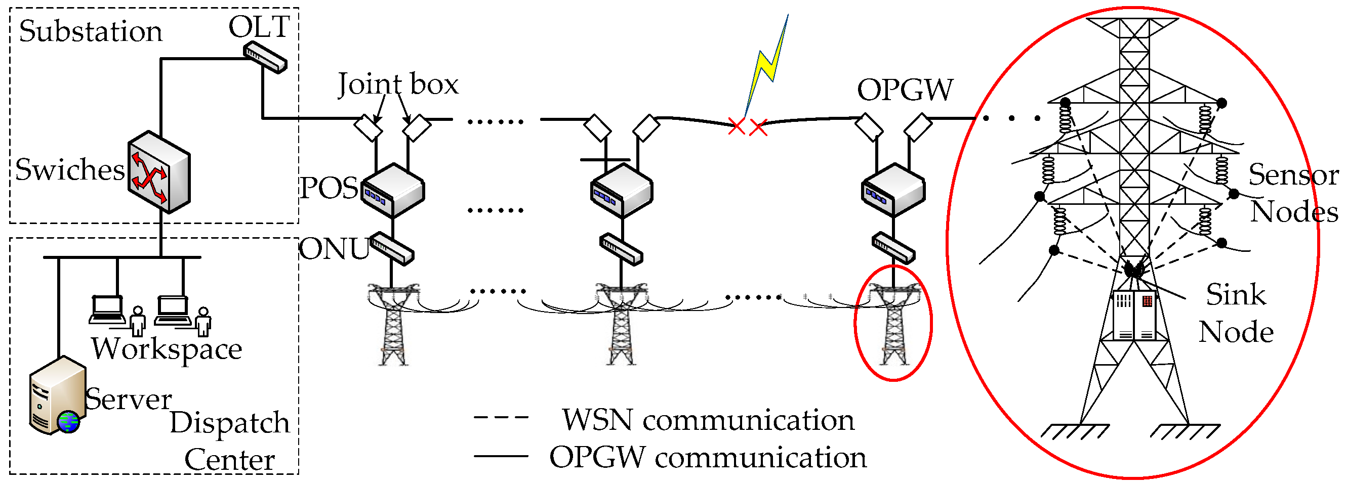
2.2. Structure of a Wireless Sensor Network-Based Monitoring System

Multilevel structure composed of hybrid communication has been proposed in several works [12,13,14,15,16] for monitoring systems. In this regard, our work is based on a practical two-layer monitoring network as shown in Figure 2. The first layer consists of sensor nodes installed at every tower. Data gathered by sensor nodes is transmitted wirelessly to a sink node by many-to-one communication. The sink node is connected to a terminal that has enhanced computation and communication. The terminal compresses monitoring data such as acceleration, tension and video and transmits them to the higher layer. The second layer is burdened with high-speed and large-data transmitting tasks. In such cases, enabling some of these towers with the capability of optical or cellular communication comes as a solution. Such a tower acts as a head in an area. This enhanced tower gathers information from sensor nodes in this area and transmits it directly to the substation. The recommended second layer in the field adopts OPGW optical-electric separation technology and an Ethernet Passive Optical Network (EPON) [23]. This communication channel is vulnerable against various forms of natural disasters and malicious physical events. In this paper, we make further study on the communication channel reconstruction and focus on these WSN modules in the first layer.

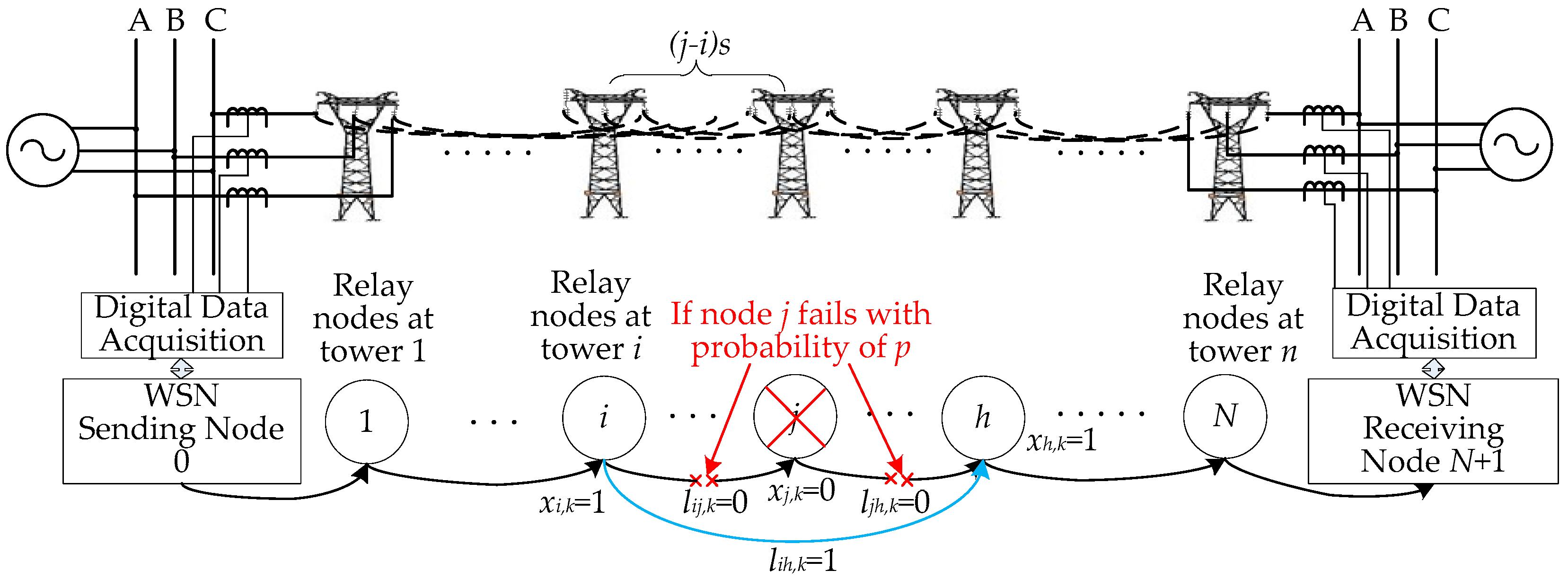
2.3. Description of Reconstructed Communication Channel Model

Figure 3 shows the RCC model between two substations. In order to focus on the research object, the external network is replaced by equivalent sources. The length of transmission line between two substations ranges from 10 to 30 km. The distance between towers can be 0.3–0.5 km according to geographic circumstances. Therefore, the possible number of towers can be 30–125.
Following the structure of the WSN-based monitoring system, the sensors placed around the towers send digital protection data from a substation to the remote one in hop-by-hop manners. The RCC model is built under the following three assumptions:
(1)
Since the communication range of radio frequency (RF) modules with the state-of-the-art is around 1 km [24], the relay can skip some adjacent nodes, e.g., from tower 1 to tower 4.
(2)
To simplify installation, sensors are placed near the tower. Then, the distance between these sensors are less than 20 m, which is far less than span distance, so nodes at a tower can be regarded as an equivalent node.
(3)
During natural disasters, the OPGW is likely to be damaged, while the WSN nodes have redundancy and most of them can survive under natural disasters. In addition, taking the self-organized characteristic of WSNs into account, they can undertake the task of transmitting protection data.

2.4. Formulation of System Arrangement

Different from monitoring communication, data is periodically generated from substations and it is an end-to-end information exchange. In such a case, there is no load imbalance issue or bottleneck issue [17] near substations. However, an optimal arrangement of the wireless sensor node for differential protection needs to be formulated considering the survivability of sensor nodes in natural disasters while satisfying the connectivity of communication networks. It is obvious that the more nodes are deployed the better. Link specific reliability can be acquired at the cost of higher complexity. Thus, there is a tradeoff between cost and reliability. In this section, an optimal arrangement formulating the placement problem is proposed while respecting all constrains.

2.4.1. Symbol Statement

The optimal arrangement scenario consists of N transmission towers. The average span and communication range in length are s and r, respectively, thus m = ⌊r/s⌋ represents the number of towers that a communication range can cover. Since the communication range covers several towers, then there are many available routes, e.g., from 1 to 3 or from 1 to 2 then to 3. To describe the route of data packets, binary variables xi,k, lij,k are used. xi,k is 1 if the end-to-end route uses the ith tower for relay in the kth route. lij,k is 1 if the data route uses a link from the ith tower to the jth tower in the kth route, and the delay of the link is described by latency tij. D represents the end-to-end delay constraints for designing. The reliability of nodes is denoted by p, indicating the contingency of the nodes’ survivability under disasters. Specifically speaking, in Figure 3, if node j fails with probability of p, then xi,k is 0 and the links related to node j are broken, that is, lij,k = 0 and ljh,k = 0. As a result of the self-healing characteristic of routing protocol, the route between node i and h is rebuilt, which is described by lih,k = 1. The number of possible routes satisfying connectivity is NR and the number of active towers through the kth route is nk, where active indicates that the tower is adopted in the kth route.

2.4.2. Optimal Arrangement Formulation

In the optimal arrangement, assuming the fixed number q of nodes needs to be deployed at each tower, the objective function of cost is shown below:
Minimize : f 1 ( q ) = c q N ,
which computes the total fixed cost for purchase and deployment of WSNs. Another consideration is the reliability of the network during natural disasters. The objective function of reliability considering network connectivity is shown in Equation (2):
Maximize : f 2 ( q , x i , k ) = k = 1 N R p e n k N R = k = 1 N R p e i = 1 N x i , k N R ,
where pe = 1 − (1 − p)q indicates the contingency of equivalent nodes’ normal working state. Considering the two objectives, a comprehensive objective function is constructed in Equation (3):
Maximize : f ( q , x i , k ) = f 2 ( q , x i , k ) f 1 ( q ) .
The comprehensive objective indicates the maximum reliability of the network per unit cost.
Constraints in Equations (4)–(9) ensure the connectivity of route and the requirement of end-to-end delay for design. Since the kth solution of these constraints corresponds to the kth route, the following constraints neglect variable k in expression for better readability:
i N j = i + 1 i + m 1 l i j = i = 0 N + 1 x i 1 i [ 0 , N + 1 ] , j [ 1 , N ] , j i ( 0 , m ] ,
x 0 = 1 , x N + 1 = 1 ,
t = i m i 1 l t i = x i , i [ 1 , N 1 ] ,
k = i + 1 i + m l i k = x i , k [ 2 , N + 1 ] ,
t ( i = 0 N + 1 x i 1 ) D , i [ 0 , N + 1 ] ,
x i , l i j { 0 , 1 } , i , j [ 0 , N + 1 ] .
Equations (4) and (5) maintain that substations are sources of protection data and one route is exactly selected for the data flow. Equations (6) and (7) ensure that if the ith tower serves as a relay node, then there are two links intersecting at tower i. Equation (8) restricts the end-to-end delay for design. If multiple latencies between the ith tower and the jth tower are imposed considering different performance of nodes, t can be replaced by tij. The last constraint in Equation (9) ensures the binary variables.

2.4.3. Monte Carlo Solution

The optimal arrangement problem can be directly solved by enumerating variables xi into Boolean strings with brute force and the complexity is o(2N). Hence, we have to weigh the computation time that a non-deterministic polynomial (NP)-complete problem will bring. To avoid unnecessary state enumeration, the Monte Carlo technique [25] is used to estimate the value of objective function after modeling the optimal arrangement problem as a probability calculation problem. Random variables x0, x1, …, xN+1 are defined as 0–1 distribution in Equation (10):
P ( x i ) = { p e x i = 1 1 p e x i = 0 .
Assuming that input variables xi are independent, the combination variable x0x1xN+1 can be generated randomly according to the probability distribution. M inputs of combination variables are generated by a Monte Carlo experiment and Ms of them are supposed to satisfy the constraints in Equations (4)–(9). The objective function in Equation (2) can be calculated by:
f 2 = M s M .

3. Overall Design of the Communication Channel Reconstruction

In this section, the overall design of the communication channel reconstruction is presented. According to the principle of the sampled-value-based and phasor-based differential protection, data preparation, communication capacity and synchronization are analyzed for the design.

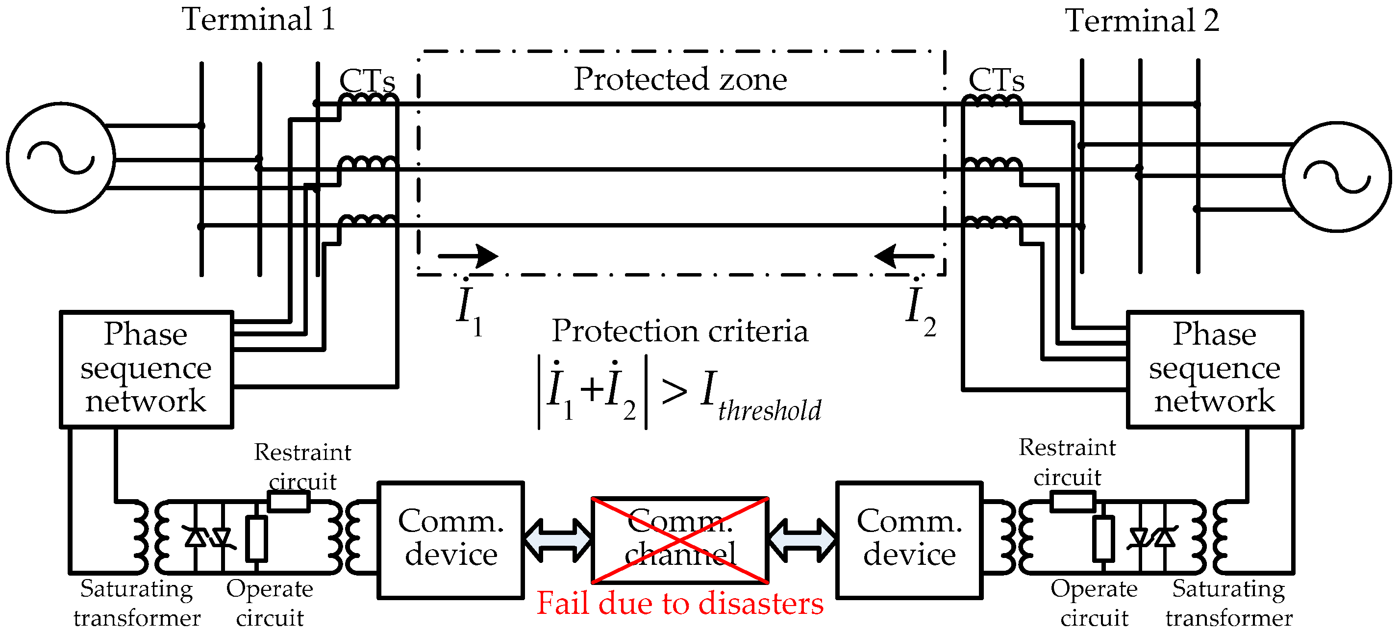
3.1. Protection Principle

The differential protection is commonly based on phasor calculation and makes a tripping decision by comparing the differential current and restraint current in phasor form. There is also a sampled-value-based differential protection adopting instantaneous values. During the steady states, the root-mean-square values of differential and restraint currents does not vary with the time window’s shifting. However, the requirements of the data packet and capacity are different for these two kinds of differential protection, which will be discussed in the following section.

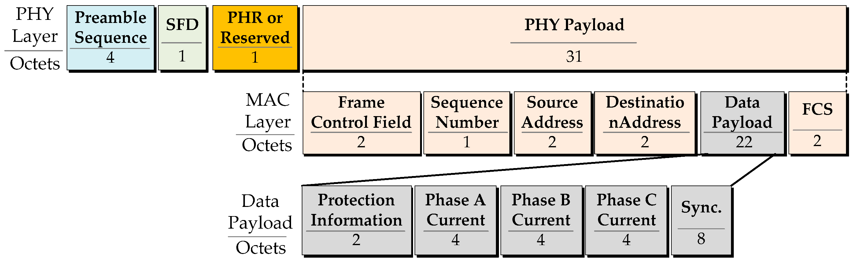
3.2. Data Preparation

The digital relay devices at each substation gather current signal obtained by current transducers and convert measured signals to digital sampled or phasor values by quantizing and encoding. The WSN data packet frame of Medium Access Control (MAC) layer launched by application layer are shown in Figure 4. The frame control field is two octets in length followed by sequence number and addressing field. The data payload has variable length and contains information on the basis of protection requirements. The digital sampled values in application layer is passed to the MAC layer as data payload. The addressing field in MAC layer is filled with a 16-bit short address, which is assigned uniquely to every node. The last field is the Frame Check Sequence (FCS), which contains a 16-bit Cyclic Redundancy Check (CRC) for transmission-error checking.
Data payload consists of protection information field, three-phase current and synchronization timestamp. The protection information field is two octets in length and contains logic and control information of the local side. In phasor-based differential protection, amplitude and angle are, respectively, quantified as 16-bit data, so each phase current is four octets in length. In sampled-value-based differential protection, each phase current can be expressed by a four-byte float-type number. In addition, the last subfield of data payload is the synchronization timestamp represented by a 64-bit unsigned fixed point number of which accuracy is about 200 picoseconds.
The MAC data frame is passed to the physical layer (PHY), which becomes the PHY payload. The PHY is prefixed with four-byte preamble (at 2.45 GHz by O-QPSK modulation), a one-byte start-of-frame delimiter (SFD) for symbol synchronization, and a one-byte frame length/reserved.

3.3. Capacity Analysis

Sampled-value and phasor criterion are used for current differential protection, both of which need to transmit corresponding current data. Assuming that sampled waveforms of current at Ns samples/cycle are adopted, the data rate of sampled-value is calculated by Equation (12):
R bs = 8 L o N s f 0 ,
where Lo is the length of PHY packet in octet and f0 is the fundamental frequency. Based on the packet frame in Figure 4, Lo is 37 octets. Therefore, to meet the IEEE 802.15.4 data rate constraints (250 kbps PHY data rate at 2.45 GHz) [26], Ns can be set as 16. If using Fourier algorithm by extracting current in a cycle data window to form a phasor, the data window will slide backward once every integer times of sampling period nTs. Specifically speaking, given 16 current values are sampled in a cycle, a new data window is constructed by adding the latest sampled current value to the end of the remaining 15 values after 1.25 ms. The data rate of phasor criterion is calculated by:
R bp = 8 L o n T s .
It can be concluded that the data rate is proportional to sampling frequency and the WSN can meet the need for both sampled-value-based and phasor-based differential protection when Ns is set to 16. Focusing on the performance of RCC for protection, the rest of this paper selects widely-adopted phasor-based differential protection for illustrative purposes.

3.4. Synchronization

To guarantee the correct action of differential protection, the current data has to be taken at the same time, and time difference between the protection relaying may lead to differential current and thus malfunctioning. In the suggested technique, Global Position System (GPS) is used for time synchronization. The two relay devices start to record the current signal after they receive pulse per second (PPS) signals and the current signals are sampled by the control of the corrected clock of crystal oscillators. In addition, the digital relays have the ability to modify the content of running data packets and each data packet storing sampled values has a corresponding timestamp in the synchronization field. The two relays on both sides continually check the synchronization field of the data packet and align the current values for differential elements.

4. Improved Routing Protocol

The routing protocols of WSN are diverse so that projects can choose a routing strategy according to their applications. To meet the need of mobile ad hoc networks (MANETs), the conventional routing protocol in WSNs is mostly derived from Ad hoc On-demand Distance Vector (AODV) routing protocol [27], which has the advantages of being on-demand and spontaneous. It initiates the route discovery when an application requests data transmission. Namely, when a route becomes invalid because of poor link quality or node damaging in natural disasters, this kind of reactive protocol initiates a next round of route discovery process to establish a new route from the source to the destination. Under this circumstance, it is the large consumption that the route discovery process introduces, especially when the network increases with the power transmission scale. However, in the application of RCC for protection, only a few hops may be broken due to the external circumstance, but others are still sound. Therefore, the representative reactive routing protocol like AODV and Dynamic Source Routing (DSR) is not suitable for protection.
In this section, a routing protocol is proposed for RCC. The advantage of this routing protocol is that routes are locally rebuilt without discovery packets flooding in the overall network. Moreover, the route assures the directional propagation of data packets will get a lower number of hops and thus result in low end-to-end delay.

4.1. Basic Concept in Route Establishment

If node S and node D are the source and destination, respectively, located at both ends of the transmission line, forward means the direction from node S to node D, and then backward means the direction from node D to node S.
In route establishment, neighbor tables of forward and backward lists are executed by any node i. The contents of route discovery neighbor table are shown in Table 1. The forward/backward list firstly describes the address of the next/previous nodes in a communication range. Distance between node i and neighboring nodes is calculated based on the GPS position information in route request messages (RREQs). Link quality indicator (LQI) describes the performance of wireless communication links. We use exponentially weighted moving-average algorithm (EWMA) [28] to calculate link quality (14):
{ P R R = N r N r + N m L Q I k + 1 = ( 1 α ) L Q I k + α P R R ,
where PRR is the packet reception rate, Nr and Nm are the number of received and missing messages respectively, and α is EWMA factor ranging from 0 to 1.

4.2. Route Discovery

4.2.1. Route Request

When the source executes a new route to a destination, it broadcasts an RREQ message containing the information of destination node and GPS position information. The RREQ can be uniquely identified by the source address and source ID number. The intermediate node receiving the RREQ firstly checks whether the request is a duplicate. If the RREQ is new, the intermediate node updates the RREQ with its GPS position information and rebroadcasts it to its neighbors. The broadcasting process is terminated when the RREQ reaches the destination.

4.2.2. Route Reply

Every node (destination node included) receiving RREQs saves GPS position information of source nodes and sends back a route reply (RREP) with its position information. The node receiving RREP will decide whether the precursor node belongs to its forward list or backward list based on the GPS position information. As shown in Figure 5, node i receives RREP from node j. Given the position vector of node I, r i = ( ϕ , λ , h ) in WGS84 (World Geodetic System 1984) coordinates parsed from RREP, the earth-centered geometric coordinate a i = ( x , y , z ) can be calculated [29]. The angle θ, defined as Equation (15), is used to describe the relative position of node i in the route map. Since the θ is a value of relative position, another variable θth is introduced to limit the range. The distance of node i and node j, denoted by dij, is calculated by Equation (16). In addition, variable dth is introduced to judge whether node i and node j are in the same tower:
θ = arccos ( a i a s ) ( a i a j ) | a i a s | | a i a j | ,
d i j = | a i a j | .
The judgment process of the forward/backward list is presented as follows:
Case 1
As shown in Figure 5a, if θ > θth, node j is added to the forward list of node i. Namely, node i is the intermediate node from the source to node j.
Case 2
As shown in Figure 5b, if θ < θth, node j is added to the backward list of node i. Namely, node j is the intermediate node from the destination to node i.
Case 3
As shown in Figure 5c, if dij < dth, node B will not be added to any list of node A. It indicates that node i and node j will not exist on the forward list or the backward list of each other when they are in the same tower range.
The threshold variables θth and dth can be set as empirical values. As a rule of thumb, θth and dth are set to 90° and 10 m, respectively. It should be mentioned that the threshold variables for some corner towers are specifically set according to geographical constraints.

4.2.3. Data Forwarding

After each node builds the routing discovery neighbor table of the forward/backward list based on their positions, the source node first sets a route option to transmit a data packet. Occupying one-bit length in the protection information field, the route option is the index of route mode. The index makes nodes on the route aware that protection is the priority and blocks the sensor collection. After setting the source route option for the data packet, the source gets the next hop to the destination node by looking up its neighbor table of the forward/backward list. The strategy of choosing the next node from the forward/backward list is given as follows: if data packets are transmitted forward, the next node should be chosen from forward list. The furthest node is chosen to decrease the number of hops based on the distance parameter in Table 1 if its LQI satisfies the required minimum link quality. If there is no node that satisfies the required minimum link quality in the list, the node with the best link quality is chosen to be the next node.

4.3. Route Maintenance

Due to extreme weather, links on a route may fail. Route maintenance is the mechanism to deal with it. It is common knowledge that a node can distinguish whether a packet is correctly received by the downstream node through acknowledgment of listening to the forwarding. Once a link fails, a link status message is specifically sent to the precursor node, and the precursor node can find out a backup link to replace it from its forward/backward list. Furthermore, when a node finds the next node fails, link status will be marked as invalid. In traditional reactive routing protocols, a link status message is sent to the source and the source starts another route discovery, which has high consumption.

4.4. Comparative Study with Other Novel Solutions

It has often been encountered that the survived nodes may still benefit us if the wireless sensor nodes remain somehow active after disasters. Aimed at this circumstance, specialized architectures of WSNs and fault-tolerant routing protocols have been proposed. Hierarchical query protocols such as low energy adaptive clustering hierarchy (LEACH) [30] and TopDisc [31] have been used in some extreme environments [32,33]. The key purpose of these protocols is choosing clusters by distributed algorithms in a hierarchical network since the node membership will dynamically change, which will force clusters to evolve over time. To assure the effective communication between each cluster, these routing protocols require that the WSNs have densely distributed nodes in a two-dimensional plane and utilize boosted clusters. However, in our application, the reconstructed communication network consists of identical nodes in elongated geographic areas. To make the routing protocol more applicable for this kind of network topology, directed diffusion protocol attracts more interest [34]. It is a non-geographic query-routing method that is based on flooding all nodes with the query, with the aim of finding every possible route from the sink and the location source, and then selecting the optimal route. This protocol is designed to reach a definite position of the network, which is suitable for our application. However, it can not prevent the construction of curved paths. Specifically speaking, there may be much meandering along the path, leading to correspondingly longer routing response time and a greater amount of battery consumption. Moreover, it does not apply to transmission of small amounts of data after receiving requests for its huge cost of route discovery.
Compared to the aforementioned novel solutions, the advantage of the proposed routing protocol is that it is a kind of table-driven routing protocol without frequent route discovery, and the route is locally rebuilt without discovery packets flooding in the overall network. Moreover, the route assures the directional propagation of data packets to get a lower number of hops, thus resulting in low end-to-end delay. Therefore, the proposed routing protocol based on geographic information may be more suitable for this application.

5. Experiments and Performance Evaluation

5.1. Performance of Monte Carlo Simulation

Based on the major components of typically battery-powered sensor nodes (BPSN), the sensor node reliability is evaluated by its radio component and microcontroller system and battery [35]. In order to reflect real scenarios, failure rate λBPSN practically acquired by statistics in normal, bad and extreme weather is 9.151 × 10⁻⁵, 1.363 × 10⁻² and 3.376 × 10⁻² failures per hour, respectively. We consider some realistic values of the parameters (p, q, r, s) = (0.4448, 2, 1000, 300) for 100 Monte Carlo experiments to show the reduction in the number of input combination that should be applied to estimate the network reliability. Assuming the failure of senor node is subjected to exponential distribution [35], the calculated sensor node reliability considering accidental failure after 24 h exposure time is 0.9978, 0.7224 and 0.4448 in normal, bad and extreme weather. The simulations are run on an Intel(R) Core(TM) i5-3470@ 3.20 GHz machine (Intel, Wuhan, China).
Table 2 illustrates the advantages of using Monte Carlo over an exhaustive experiment for different percentage errors. If we can tolerate 0.1 percent error for network reliability, around ten thousand input combinations have to be applied. If we can tolerate one percent error for network reliability, we have to apply a total of around a thousand input combinations. In addition, when the number of towers is very high (greater than 15), Monte Carlo proves to be very effective. In the following cases, we apply 105 input combinations, which is enough to meet the accuracy for optimal arrangement.

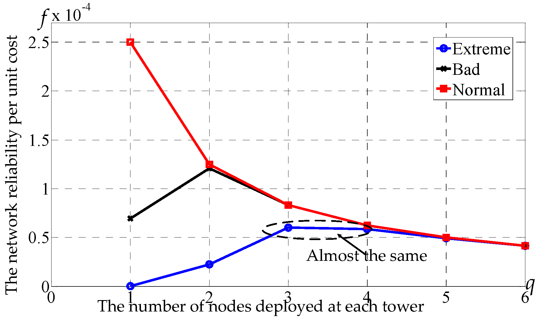
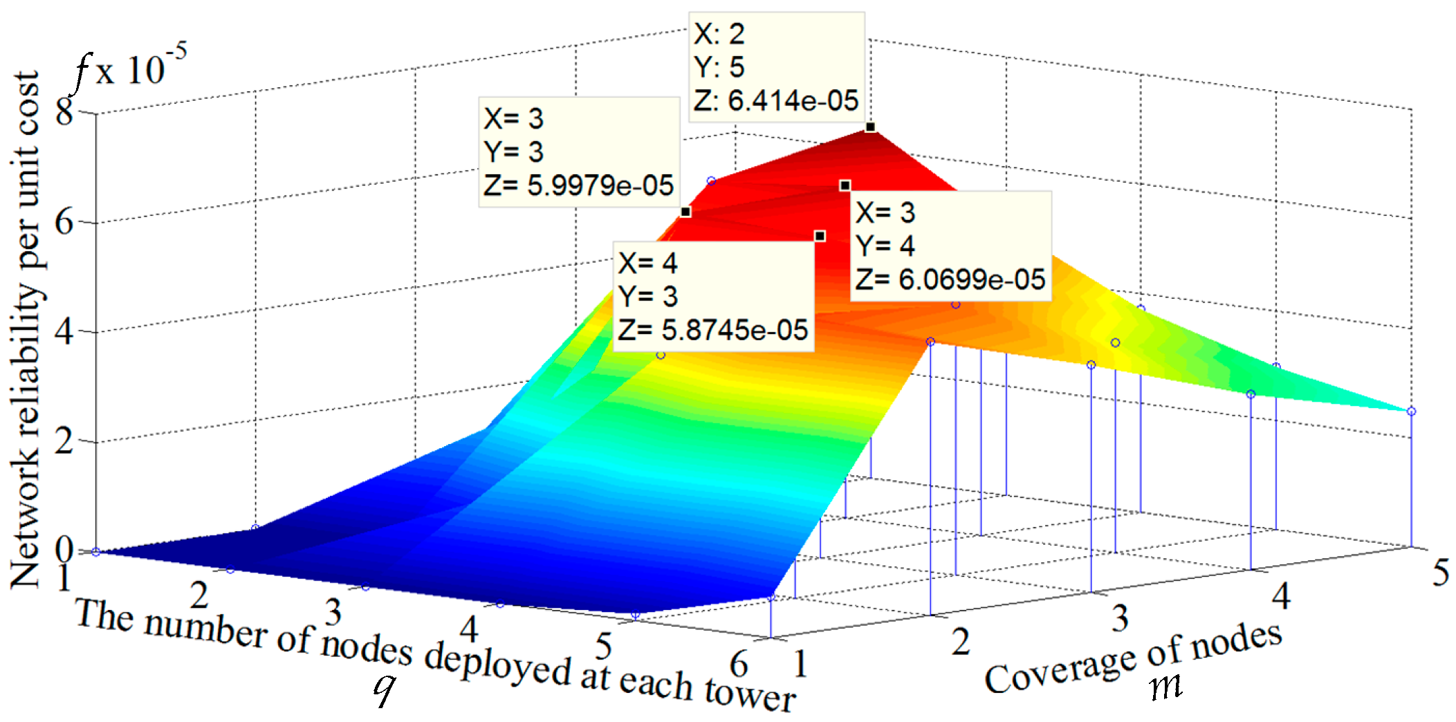
5.2. Effect of the Number of Nodes Deployed at Each Tower

Figure 6 shows the effect of the number of nodes at each tower on the network reliability per unit cost. We consider a simulation of an 80-tower network in normal, bad and extreme weather. The price of 1000 m communication-range node is $50. The cost increases approximately linearly with respect to the number of nodes deployed at each tower, but the reliability has a slower incensement. For any given network and a certain type of sensor nodes, this graph can be used to find the most cost effective arrangement. In this case, the optimal number of nodes deployed at each tower is one, two and three for normal, bad and extreme weather. Generally, we consider three nodes in each tower for conservation design.
It should be mentioned that sometimes planners tend to value the network reliability above cost. Especially in this case, three-node arrangement in extreme weather is almost as cost effective as four-node arrangement, but the network reliability in four-node arrangement (0.9398) is much higher than three-node arrangement (0.7206). Therefore, four-node arrangement is more acceptable. This analysis can be a decision aid in obtaining the optimal number of nodes in network planning.

5.3. Effect of Communication Range

The network reliability and cost is not only related to the number of nodes deployed at each tower but is also related to communication range of nodes. To comprehensively illustrate the tradeoff between cost and reliability in extreme weather, we consider an 80-tower network consisting of five practical types of nodes that has different RF modules and thus different prices (Table 3). Figure 7 shows the effect of the communication range with respect to network reliability per unit cost. In the case of fixed node cost, the total cost grows with an increasing number of nodes deployed at each tower. In the case of adaptive node cost depending upon communication range, total costs increase rapidly if using better nodes. Thus, it can be profitable to deploy nodes according to the network reliability per unit cost. According to results in Table 3, deploying two five-tower coverage nodes at each tower is suggested.

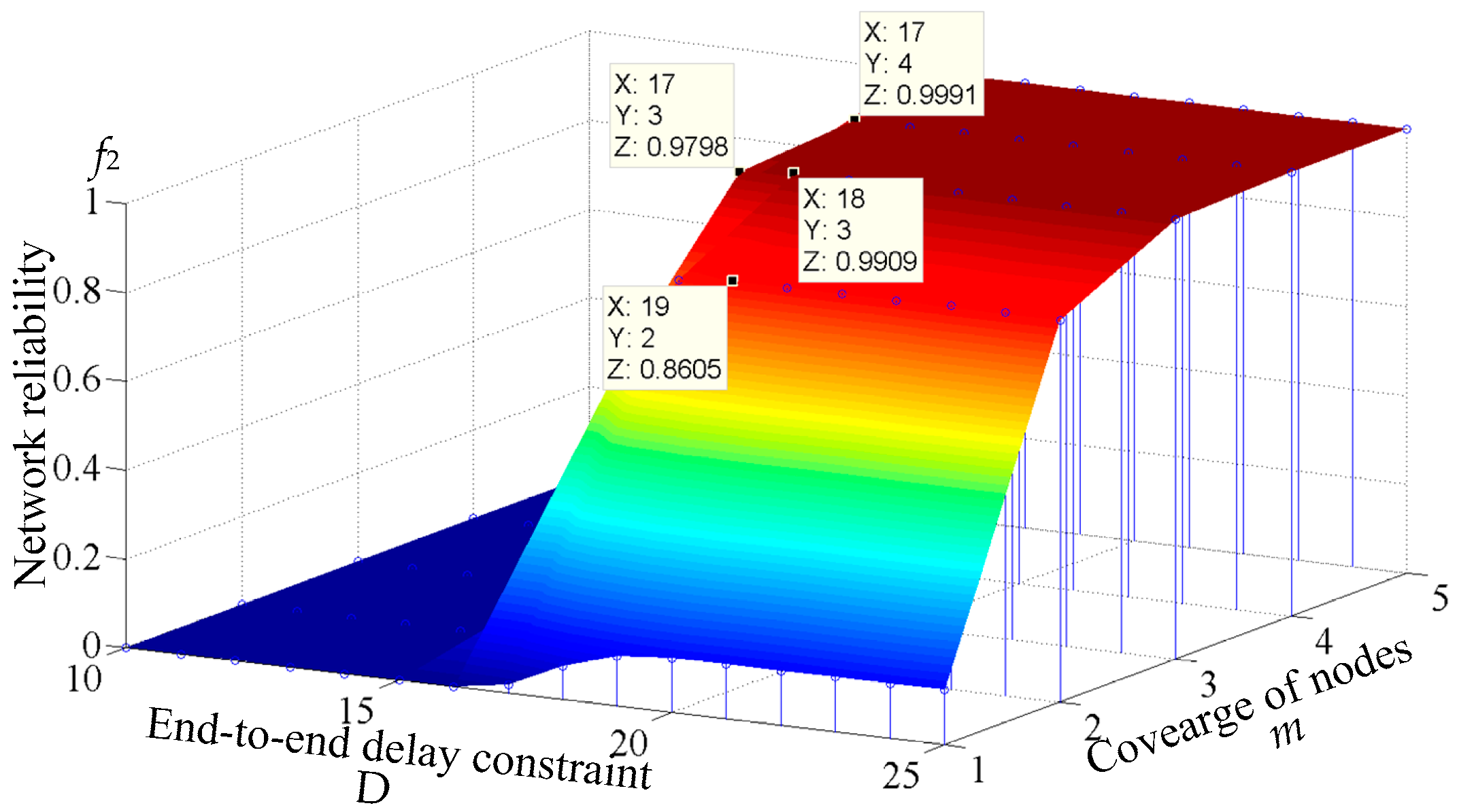
5.4. Effect of End-to-End Delay Constraint

In the optimal arrangement, some possible routes may not satisfy the end-to-end delay constraint, which results in low network reliability. The most effective way is adopting nodes with a large communication range. Assuming the end-to-end delay is mainly caused by multi-hopping and not accounting for queuing delay or channel collision, the latency incurred due to links is 1.2 ms [26]. Figure 8 shows the effect of end-to-end delay constraint when two nodes are deployed at each tower. Given a small deadline requirement to get a quick action of protection, it results in large-communication-range nodes being used. Notice in the graph that the communication range should cover two towers or above to achieve acceptable network reliability (over 0.9). For a given constraint, this graph can be used to choose the communication range of nodes and acquire acceptable reliability.

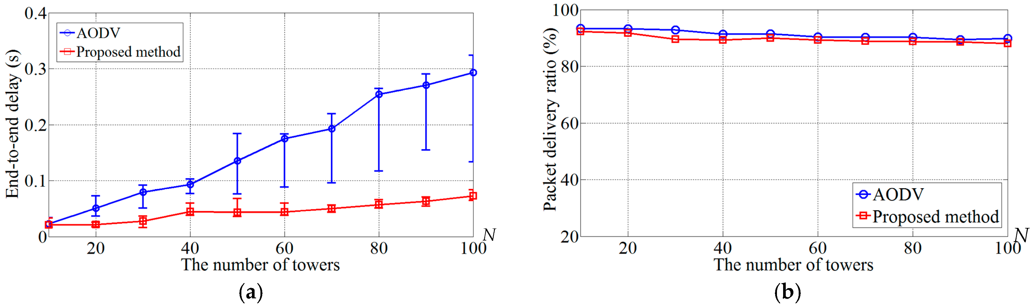
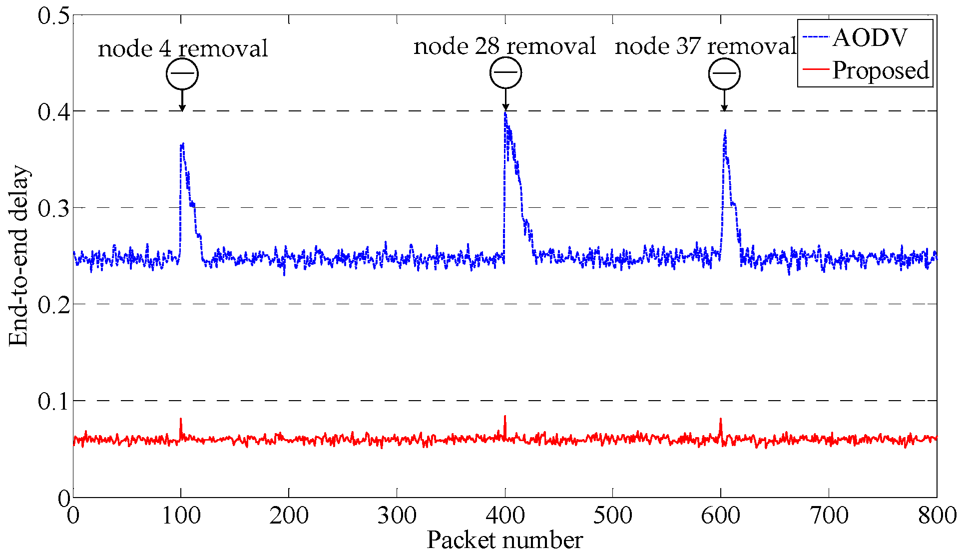
5.5. Performance of the Routing Protocol

In this section, we evaluate the proposed routing protocol in some metric of the RCC performance. Compared with conventional AODV routing protocol, the evaluation analysis includes end-to-end delay and packet delivery ratio. In this simulation, the NS-2 and IEEE 802.15.4 PHY/MAC protocol are used. All the statistics of the evaluation are acquired from the packet–trace report of NS2. We use WSN as a transparent medium that passes CBR (constant bit rate) traffic. The maximum receiving range and carrier sensing range are 1600 and 3520 m, respectively. There are 80 towers in the network. The neighbor tables of the forward and backward list are created by the link status message with one-hop broadcast.
The end-to-end delay of AODV significantly increases to 0.3 s with the number of nodes increasing, as shown in Figure 9a. The main reasons are repeated routing request time and overlapped routing paths. On the other hand, the proposed method shows low end-to-end delay compared with AODV, since the proposed method has no other round of route discovery before transmitting data. As for the packet delivery ratio in Figure 9b, the proposed method is comparable to AODV because the network congestion causing collision and drops of the packets of AODV is comparable to the proposed routing protocol.
Figure 10 evaluates the proposed routing protocol after the removal of some nodes. A removal of a key relay node leads to initiations of the next route discovery for AODV, which results in high end-to-end delay of the coming data packet. In this case, the proposed method can quickly recover the broken route.

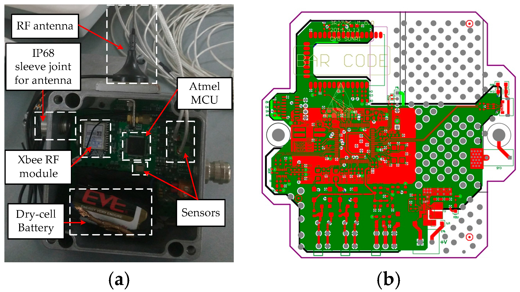
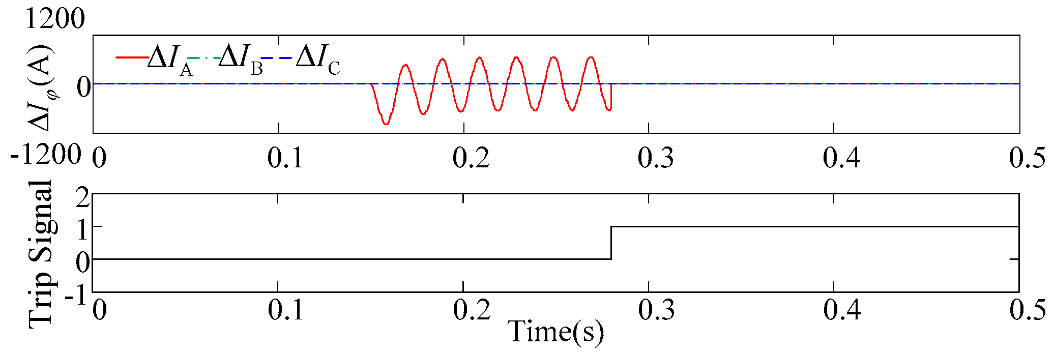
5.6. Experimental Test

To verify the proposed scheme and its performance, WSN nodes and devices have been developed (Figure 11) and deployed along a 25 km transmission line in Guangzhou Province to build RCC. A single-phase-to-ground fault happens at 0.16 s and the recorded differential current of each phase is shown in Figure 12. The trip signal is activated at 0.2813 s, which takes 121.3 ms since the fault happens. The time consumption takes end-to-end latency into account as well as the protection algorithm cost. Although the time delay is longer than optical-fiber based communication, it is acceptable as an emergency communication channel under the condition that the main communication channel fails.

6. Conclusions

In this paper, an emergency communication channel reconstruction scheme was presented. An optimal system arrangement for a cost-reliability balanced wireless network was formulated. The effects of the number of nodes deployed at each tower, communication range and end-to-end delay constraint were analyzed, which can be a decision aid in network planning. In addition, a novel routing protocol for WSNs was proposed to meet the protection speed. We compare the performance with the AODV routing protocol. The analysis showed that the proposed method can quickly recover the broken route without another round of route discovery process, and therefore low end-to-end delay will occur within. Furthermore, the effectiveness of the RCC was validated by experimental tests.
Limitations of the proposed routing protocol have been revealed in some complex situations such as multiple-circuit crossover overhead transmission lines. In this case, the current signals measured at both ends, respectively, should be adopted for differential protections of these two transmission lines. However, the proposed routing discovery process is based on the geographical information by assuming that WSN nodes are deployed along elongated areas. Therefore, under this circumstance, the proposed route discovery process may not distinguish the direction of data flow if the threshold variable θth is not appropriately chosen. In practice, the WSN nodes’ group identification was specifically configured in this area to solve this problem; however, it was not automated, and secondary hardware and software programming for nodes were needed. To this end, automatically selecting waypoints in this specific situation using heuristic methods and classification techniques may be a future key research issue.

Acknowledgments

This work is supported in part by the National High Technology Research and Development of China (863 Program): No. 2015AA050201.

Author Contributions

Xu Chen and Xianggen Yin conceived and wrote the paper; Xu Chen and Bin Yu performed and analyzed the experiments; Zhe Zhang contributed analysis tools.

Conflicts of Interest

The authors declare no conflict of interest.

References

  1. Miao, S.H.; Liu, P.; Lin, X. An adaptive operating characteristic to improve the operation stability of percentage differential protection. IEEE Trans. Power Deliv. 2010, 25, 1410–1417. [Google Scholar] [CrossRef]
  2. Blackburn, J.L.; Domin, T.J. Protective Relaying: Principles and Applications, 3rd ed.; CRC Press: Boca Raton, FL, USA, 2007. [Google Scholar]
  3. Lin, X.; Tian, Q.; Zhao, M. Comparative analysis on current percentage differential protections using a novel reliability evaluation criterion. IEEE Trans. Power Deliv. 2006, 21, 66–72. [Google Scholar] [CrossRef]
  4. IEEE Guide for Power System Protective Relay Applications over Digital Communication Channels; C37.236–2013; IEEE Std.: New York, NY, USA, 2013.
  5. Li, H.; Rosenwald, G.W.; Jung, J.; Liu, C. Strategic power infrastructure defense. IEEE J. 2005, 93, 918–933. [Google Scholar]
  6. Asea Brown Boveri Ltd. Line Differential Protection RED 670 2.0 IEC Application Manual; Asea Brown Boveri Ltd.: Hong Kong, China, 2014. [Google Scholar]
  7. Ryutaro, K. Architectures for ATM network survivability. IEEE Commun. Surv. 1998, 1, 2–11. [Google Scholar]
  8. Fodero, K.; Rosselli, G. Applying Digital Current Differential Systems over Leased Digital Service. In Proceedings of the 58th Annual Conference for Protective Relay Engineers, College Station, TX, USA, 5–7 April 2005; pp. 291–298.
  9. Zhang, P.; Li, F.; Bhatt, N. Next-generation monitoring, analysis, and control for the future smart control center. IEEE Trans. Smart Grid 2010, 1, 186–192. [Google Scholar] [CrossRef]
  10. Gungor, V.C.; Lambert, F.C. A survey on communication networks for electric system automation. Comput. Netw. 2006, 50, 877–897. [Google Scholar] [CrossRef]
  11. Bose, A. Smart transmission grid applications and their supporting infrastructure. IEEE Trans. Smart Grid 2010, 1, 11–19. [Google Scholar] [CrossRef]
  12. Yang, Y.; Divan, D.; Harley, R.G.; Habetler, T.G. Design and Implementation of Power Line Sensornet for Overhead Transmission Lines. In Proceedings of the 2009 IEEE Power and Energy Society General Meeting, Calgary, AB, Canada, 26–30 July 2009.
  13. Li, F.; Qiao, W.; Sun, H.; Wan, H.; Wang, J.; Xia, Y.; Xu, Z.; Zhang, P. Smart transmission grid: Vision and framework. IEEE Trans. Smart Grid 2010, 1, 168–177. [Google Scholar] [CrossRef]
  14. Gungor, V.C.; Lu, B.; Hancke, G.P. Opportunities and challenges of wireless sensor networks in smart grid—A case study of link quality assessments in power distribution systems. IEEE Trans. Ind. Electron. 2010, 57, 3557–3564. [Google Scholar] [CrossRef]
  15. Fateh, B.; Govindarasu, M.; Ajjarapu, V. Wireless network design for transmission line monitoring in smart grid. IEEE Trans. Smart Grid 2013, 4, 1076–1086. [Google Scholar] [CrossRef]
  16. Wu, Y.; Cheung, L.; Lui, K.; Pong, P. Efficient communication of sensors monitoring overhead transmission lines. IEEE Trans. Smart Grid 2012, 3, 1130–1136. [Google Scholar] [CrossRef] [Green Version]
  17. Abdel-Latif, K.M.; Eissa, M.M.; Ali, A.S.; Malik, O.P.; Masoud, M.E. Laboratory investigation of using Wi-Fi protocol for transmission line differential protection. IEEE Trans. Power Deliv. 2009, 24, 1087–1094. [Google Scholar] [CrossRef]
  18. Hung, K.S.; Lee, W.K.; Li, V.O.K.; Lui, K.S.; Pong, P.W.T.; Wong, K.K.Y.; Yang, G.H.; Zhong, J. On wireless sensors communication for overhead transmission line monitoring in power delivery systems. In Proceedings of the 2010 IEEE International Conference on Smart Grid Communications, Gaithersburg, MD, USA, 4–6 October 2010; pp. 309–314.
  19. North American Electric Reliability Council. 2000 System Disturbances Review of Selected Electric System Disturbances in North America; North American Electric Reliability Council: Atlanta, GA, USA, 2000. [Google Scholar]
  20. Italian Government Working Group on Critical Information Infrastructure Protection (PIC). La Protezione delle Infrastrutture Critiche Informatizzate—La Realtá Italiana; Italian Government: Rome, Italy, 2004. (In Italian)
  21. Chen, Q.; Yin, X.; You, D.; Hou, H.; Tong, G.; Wang, B.; Liu, H. Review on Blackout Process in China Southern Area Main Power Grid in 2008 Snow Disaster. In Proceedings of the 2009 IEEE Power & Energy Society General Meeting, Calgary, AB, Canada, 26–30 July 2009.
  22. Hou, H.; Yin, X.; Chen, Q.; Tong, G.; You, D.; Wang, B.; He, X.; Liu, H. Analysis of Vulnerabilities in China’s Southern Power System Using Data from the 2008 Snow Disaster. In Proceedings of the 2009 IEEE Power & Energy Society General Meeting, Calgary, AB, Canada, 26–30 July 2009.
  23. Chen, X.; Du, Z.; Yin, X.G.; Pan, W.; Xu, L.Q. A Design of WSN and EPON applied in online monitoring for transmission line. Adv. Mater. Res. 2014, 950, 125–132. [Google Scholar] [CrossRef]
  24. Digi International Inc. Xbee-pro 2009. Available online: http://www.digi.com (accessed on 26 September 2016).
  25. Binder, K.; Heermann, D.W. Monte Carlo Simulation in Statistical Physics; Springer: New York, NY, USA, 1997; pp. 5–7. [Google Scholar]
  26. IEEE Standard for Information Technology—Part 15.4: Wireless Medium Access Control and Physical Layer Specifications for Low Rate Wireless Personal Area Networks; IEEE 802.15.4–2006; IEEE: New York, NY, USA, 2006.
  27. Perkins, C.E.; Royer, E.M. Ad-hoc On-Demand Distance Vector Routing. In Proceedings of the Workshop Mobile Computing Systems and Applications, New Orleans, LA, USA, 25–26 February 1999.
  28. Shu, J.; Liu, L.; Zhang, R. An Energy-Effective Link Quality Monitoring Mechanism for Event-Driven Wireless Sensor Network. In Proceedings of the WRI International Conference Communications and Mobile Computing, Yunnan, China, 6–8 January 2009; pp. 111–115.
  29. King, C. Virtual Instrumentation-Based System in a Real-Time Applications of GPS/GIS. In Proceedings of the International Conference on Recent Advances in Space Technologies, Istanbul, Turkey, 20–22 November 2003; pp. 403–408.
  30. Makwana, N.D.; Kumar, A. Virtual Cluster Head-Set Based Avalanche Predication in Himalayan Region. In Proceedings of the 2014 International Conference on Advanced Communication Control and Computing Technologies, Ramanathapuram, India, 8–10 May 2014.
  31. Deb, B.; Bhatnagar, S.; Nath, B. A Topology Discovery Algorithm for Sensor Networks with Applications to Network Management; DCS Technical Report DCS-TR-411; Rutgers University: New Brunswick, NJ, USA, 2001. [Google Scholar]
  32. Heinzelman, W.B.; Chandrakasan, A.P.; Balakrishnan, H. An application-specific protocol architecture for wireless microsensor networks. IEEE Trans. Wirel. Commun. 2002, 1, 660–670. [Google Scholar] [CrossRef]
  33. Al-Nabhan, N.; Al-Rodhaan, M.; Al-Dhelaan, A. Cooperative approaches to construction and maintenance of networks’ virtual backbones for extreme wireless sensor applications. IEEE Sens. J. 2014, 14, 3782–3790. [Google Scholar] [CrossRef]
  34. Liu, J.; Ping, Z. Fault Tolerant and Storage Efficient Directed-Diffusion for Wireless Sensor Networks. In Proceedings of the 2010 IEEE International Conference on Information Theory and Information Security, Beijing, China, 17–19 December 2010; pp. 884–887.
  35. Zonouz, A.E.; Sun, Y.; Xing, L.; Vokkarane, V.M. Hybrid wireless sensor networks: A reliability, cost and energy-aware approach. IET Wirel. Sens. Syst. 2016, 6, 42–48. [Google Scholar] [CrossRef]
Figure 1. Functional setup of current differential protection.
Energies 09 00893 g001
Figure 2. Practical structure of a wireless-sensor-networks (WSN)-based monitoring system.
Energies 09 00893 g002
Figure 3. Description of reconstructed communication channel (RCC) model by hop-by-hop relaying.
Energies 09 00893 g003
Figure 4. WSN data packet frame.
Energies 09 00893 g004
Figure 5. Schematic diagram of forward/backward judgment. (a) forward list; (b) backward list; and (c) nodes in short range.
Energies 09 00893 g005
Figure 6. Effect of the number of nodes deployed at each tower.
Energies 09 00893 g006
Figure 7. Effect of communication range.
Energies 09 00893 g007
Figure 8. Effect of end-to-end delay constraint.
Energies 09 00893 g008
Figure 9. Routing Protocol performance different network scale. (a) average, maximum and minimum end-to-end delay; and (b) packet delivery ratio.
Energies 09 00893 g009
Figure 10. Routing protocol performance with node removal.
Energies 09 00893 g010
Figure 11. Experimental prototype of wireless sensor devices. (a) wireless sensor node in shell; and (b) and printed circuit board (PCB) design of wireless sensor module.
Energies 09 00893 g011
Figure 12. Differential current of each phase and the trip signal (single-phase-to-ground fault happens at 0.16 s).
Energies 09 00893 g012
Table 1. Route discovery neighbor table of the forward/backward list.
Address of NodesDistanceLink Quality Indicator (LQI)Link Status
Address 1d1LQI1Valid/invalid
Address ndnLQInValid/invalid
Table 2. Comparison between Monte Carlo and an exhaustive experiment.
NMonte Carlo ExperimentsExhaustive Simulations
ε = 1%ε = 0.1%Network ReliabilityTime (s)
Number of InputsTime (s)Number of InputsTime (s)
101.3 × 1030.230969.3 × 1031.293380.833730.09567
155.8 × 1030.805952.1 × 1042.934540.747362.35184
205.2 × 1030.763251.8 × 1042.759170.6699476.6096
256.2 × 1031.754632.9 × 1044.310000.600542569.68
307.5 × 1032.228553.1 × 1044.590220.5383385,312.1
Table 3. Communication Range@ 2.4GHz and prices of sensor node devices.
Types 1DTK DRF1601ATZGB-780F1Xbee-ZB SMTXbee-PRODTK DRF1605H
RF Range<400 m<750 m<1200 m<1500 m≥1600 m
Coverage of nodes 212345
Price 3$25$39$50$65$84
ProducerDTK Electronics (Shenzhen, China)Atmel (San Jose, CA, USA)Digi (Minnetonka, MN, USA)Digi (Minnetonka, MN, USA)DTK Electronics (Shenzhen, China)
Notes: 1 The types of sensor node is based on some Zigbee node makers and suppliers. It indicates available devices or systems on chip; 2 The coverage of nodes means the number of tower in communication range; 3 The price of sensor node devices depends mainly on the microcontroller Units (MCUs), radio frequency (RF) modules and Printed Circuited Board (PCB) manufacture. In this case, we only study the difference of RF modules assuming other factors are the same.

