Application of Hybrid Quantum Tabu Search with Support Vector Regression (SVR) for Load Forecasting

Abstract

Hybridizing chaotic evolutionary algorithms with support vector regression (SVR) to improve forecasting accuracy is a hot topic in electricity load forecasting. Trapping at local optima and premature convergence are critical shortcomings of the tabu search (TS) algorithm. This paper investigates potential improvements of the TS algorithm by applying quantum computing mechanics to enhance the search information sharing mechanism (tabu memory) to improve the forecasting accuracy. This article presents an SVR-based load forecasting model that integrates quantum behaviors and the TS algorithm with the support vector regression model (namely SVRQTS) to obtain a more satisfactory forecasting accuracy. Numerical examples demonstrate that the proposed model outperforms the alternatives.

1. Introduction

A booming economy is dramatically increasing electric loads in every industry and those associated with people’s daily lives. Meeting the demand of all has become an important goal of electricity providers. However, as mentioned by Bunn and Farmer [1], a 1% increase in the error in an electricity demand forecast corresponds to a £10 million increase in operating costs. Therefore, decision-makers seek accurate load forecasting to set effective energy policies, such as those concerning new power plants and investment in facilities [2]. Importing or exporting electricity in energy-limited developing economies, such as that of Taiwan, is almost impossible [3,4]. Unfortunately, electric load data have various characteristics, including nonlinearity and chaos. Moreover, many exogenous factors interact with each other, affecting forecasting, such as economic activities, weather conditions, population, industrial production, and others. These effects increase the difficulty of load forecasting [5].

In the last few decades, models for improving the accuracy of load forecasting have included the well-known Box–Jenkins’ ARIMA model [6], exponential smoothing model [7], Kalman filtering/linear quadratic estimation model [8,9,10], the Bayesian estimation model [11,12,13], and regression models [14,15,16]. However, most of these models are theoretically based on assumed linear relationships between historical data and exogenous variables and so cannot effectively capture the complex nonlinear characteristics of load series, or easily provide highly accurate load forecasting.

Since the 1980s, to improve the accuracy of load forecasting, many artificial intelligent (AI) approaches have been used and been combined to develop powerful forecasting methods, such as artificial neural networks (ANNs) [17,18,19,20,21], expert system-based methods [22,23,24], and fuzzy inference approaches [25,26,27,28]. Recently, these AI approaches have been hybridized with each other to provide more accurate forecasting results [29,30,31,32,33], with the aforementioned linear models [34], or with evolutionary algorithms [35,36]. However, the shortcomings of these AI approaches include the need to determine the structural parameters [37,38], the time required for knowledge acquisition [39], and a lack of correct and consistent heuristic rules to generate a complete domain knowledge base [40]. Extensive discussions of load forecasting models can be found elsewhere [41].

In the middle of the 1990s, support vector regression (SVR) [42] began to be used to solve forecasting problems [43], and in the 2000s, Hong et al. [44,45,46,47,48,49,50,51,52,53,54,55,56] developed various SVR-based load forecasting models by hybridizing evolutionary algorithms, chaotic mapping functions and cloud theory with an SVR model, to effectively determine its three parameters to improve the forecasting accuracy. Based on Hong’s research results, the accurate determination of three parameters of the SVR model is critical to improving its forecasting performance. The drawbacks of evolutionary algorithms cause the combination of parameters during the optimal modeling process, such as premature convergence or trapping in a local optimum. Therefore, Hong and his colleagues investigated the possibility of using chaotic mapping functions to increase the ergodicity over the search space, then transfer the three parameters into chaotic space to make the search more compact, and employ the cloud theory to establish a cooling mechanism during annealing process to enrich the influent effects of temperature decreasing mechanism, and eventually, improve the searching quality of SA algorithm for better forecasting accuracy.

Inspired by the excellent work of Hong et al., the authors find that the tabu search (TS) [57,58] algorithm is simply implemented to iteratively find a near-optimal solution, so it is powerful and has been successfully used to solve various optimization problems [59,60,61]. The TS algorithm, even with a flexible memory system to record recently visited solutions, and the ability to climb out of local minima, suffers from the tuning of the tabu tenure, meaning that it still becomes stuck at local minima and has a low convergence speed [62,63]. Also, the best solution is fixed for long iterations, i.e., it takes a great deal of time to escape to near-global optima from current position [64]. Therefore, both intensification and diversification strategies should be considered to improve the robustness, effectiveness and efficiency of simple TS; a more powerful neighborhood structure can be feasibly constructed by applying quantum computing concepts [65]. The same old problem, premature convergence or trapping at local optima, causes the forecasting accuracy to be unsatisfactory. This paper seeks to extend Hong’s exploration to overcome the shortcomings of the TS algorithm, and to use the improved TS algorithm to forecast electric loads.

In this work, quantum computing concepts are utilized to improve the intensification and diversification of the simple TS algorithm; to improve its searching performance, and thus to improve its forecasting accuracy. The forecasting performance of the proposed hybrid quantum TS algorithm with an SVR model—the support vector regression quantum tabu search (SVRQTS) model—is compared with that of four other forecasting methods that were proposed by Hong [56] and Huang [66]. This paper is organized as follows. Section 2 presents the detail processes of the proposed SVRQTS model. The basic formulation of SVR and the quantum tabu search (QTS) algorithm are introduced. Section 3 presents two numerical examples and compares published methods with respect to forecasting accuracy. Finally, Section 4 draws conclusions.

2. Methodology of Support Vector Regression Quantum Tabu Search (SVRQTS) Model

2.1. Support Vector Regression (SVR) Model

A brief introduction of an SVR model is provided as follows. For a given training data set, $G={\left\{(x_i,y_i)\right\}}_{i=1}^n$, where $x_i$ is a vector of fed-in data and $y_i$ is the corresponding actual values. G is then mapped into a high dimensional feature space by a nonlinear mapping function, $\mathsf{\phi }(\cdot )$. Theoretically, in the feature space, there should be an optimized linear function, f, to approximate the relationship between $x_i$ and $y_i$. This kind of optimized linear function is the so-called SVR function and is shown as Equation (1),

$$f(x)=w^T\mathsf{\phi }(x)+b$$

(1)

where $f(x)$ represents the forecasting values; the coefficients w and b are coefficients which are estimated by minimizing the empirical risk function as shown in Equation (2),

$$\begin{gathered} R(f)=\frac{1}{N}{\displaystyle \sum _{i=1}^N{L}_{\mathsf{\epsilon }}(y_i,w^T\mathsf{\phi }(x)+b)}+\frac{1}{2}{w}^{T}w \\ {L}_{\mathsf{\epsilon }}(y,f(x))=\{\begin{array}{cc}\left|f(x)-y\right|-\mathsf{\epsilon },& \mathrm{if}\left|f(x)-y\right|\ge \mathsf{\epsilon }\\ 0,& \mathrm{otherwise}\end{array} \end{gathered}$$

(2)

where $L_{\mathsf{\epsilon }}(y,f(x))$ is the $\mathsf{\epsilon }$-insensitive loss function. The $\mathsf{\epsilon }$-insensitive loss function is employed to find out an optimum hyper plane on the high dimensional feature space to maximize the distance separating the training data into two subsets. Thus, the SVR focuses on finding the optimum hyper plane and minimizing the training error between the training data and the $\mathsf{\epsilon }$-insensitive loss function. The SVR model then minimizes the overall errors as shown in Equation (3),

$$\begin{gathered} \underset{w,b,{\mathsf{\xi }}^{*},\mathsf{\xi }}{\mathrm{Min}}R(w,{\mathsf{\xi }}^{*},\mathsf{\xi })=\frac{1}{2}{w}^{T}w+C{\displaystyle \sum _{i=1}^N({\mathsf{\xi }}_{\mathrm{i}}^{*}{+\mathsf{\xi }}_{\mathrm{i}})}\text{ with the constraints}: \\ \begin{array}{ll}{y}_i-w^T\mathsf{\phi }(x_i)-b\le \mathsf{\epsilon }+{\mathsf{\xi }}_i^{*},\hfill & i=1,2,\mathrm{...},N\hfill \\ -y_i+w^T\mathsf{\phi }(x_i)+b\le {\mathsf{\epsilon }+\mathsf{\xi }}_i,\hfill & i=1,2,\mathrm{...},N\hfill \\ {\mathsf{\xi }}_i^{*}\ge 0,\hfill & i=1,2,\mathrm{...},N\hfill \\ {\mathsf{\xi }}_i\ge 0,\hfill & i=1,2,\mathrm{...},N\hfill \end{array} \end{gathered}$$

(3)

The first term of Equation (3), by employing the concept of maximizing the distance of two separated training data, is used to regularize weight sizes, to penalize large weights, and to maintain regression function flatness. The second term, to penalize the training errors of $f(x)$ and y, decides the balance between confidence risk and experience risk by using the $\mathsf{\epsilon }$-insensitive loss function. C is a parameter to specify the trade-off between the empirical risk and the model flatness. Training errors above $\mathsf{\epsilon }$ are denoted as ${\mathsf{\xi }}_i^{*}$, whereas training errors below $-\mathsf{\epsilon }$ are denoted as ${\mathsf{\xi }}_i$, which are two positive slack variables, representing the distance from actual values to the corresponding boundary values of $\mathsf{\epsilon }$-tube.

After the quadratic optimization problem with inequality constraints is processed, the parameter vector w in Equation (1) is obtained in Equation (4),

$$w={\displaystyle \sum _{i=1}^N\left({\mathsf{\beta }}_i^{*}-{\mathsf{\beta }}_i\right)\mathsf{\phi }(x_i)}$$

(4)

where ${\mathsf{\beta }}_i^{*}$, ${\mathsf{\beta }}_i$, satisfying the equality ${\mathsf{\beta }}_i{*\mathsf{\beta }}_i^{*}=0$, are the Lagrangian multipliers. Finally, the SVR regression function is obtained as Equation (5) in the dual space,

$$f(x)={\displaystyle \sum _{i=1}^N\left({\mathsf{\beta }}_i^{*}-{\mathsf{\beta }}_i\right)K(x_i,x)}+b$$

(5)

where $K(x_i,x_j)$ is so-called the kernel function, and the value of the kernel equals the inner product of two vectors, $x_i$ and $x_j$, in the feature space $\mathsf{\phi }(x_i)$ and $\mathsf{\phi }(x_j)$, respectively; that is, $K(x_i,x_j)=\mathsf{\phi }(x_i)\cdot \mathsf{\phi }(x_j)$. However, the computation of the inner product in the high feature space becomes a computationally complicated problem along with the increase in the input dimensions. Such a problem of contradiction between high dimensions and computational complexity can be overcome by using the kernel trick or defining appropriate kernel functions in place of the dot product of the input vectors in high-dimensional feature space. The kernel function is used to directly compute the inner product from the input space, rather than in the high dimensional feature space. Kernel functions provide a way to avoid the curse of dimensionality. There are several types of kernel function, and it is hard to determine the type of kernel functions for specific data patterns [67]. The most commonly used kernel functions include linear functions, polynomial functions, Gaussian functions, sigmoid functions, splines, etc. The Gaussian function, $K(x_i,x_j)=\exp \left(-0.5{\Vert x_i-x_j\Vert }^2/{\mathsf{\sigma }}^2\right)$, is used widely among all these various kernel functions as it can map the input space sample set into a high dimensional feature space effectively and is good for representing the complex nonlinear relationship between the input and output samples. Furthermore, only one variable (the width parameter, σ) is there to be defined. Considering the above advantages, the Gaussian radial basis function (RBF) is employed as the kernel function in this study.

The most important consideration in maximizing the forecasting accuracy of an SVR model is the well determination of its three parameters, which are the hyper-parameters, C, ε, and the kernel parameter, σ. Therefore, finding efficient algorithms for evaluating these three parameters is critical. As indicated above, inspired by Hong’s hybridization of chaotic mapping functions with evolutionary algorithms to find favorable combinations of parameters and to overcome the premature convergence of the evolutionary algorithms, this work uses another (quantum-based) method to find an effective hybrid algorithm without the drawbacks of the TS algorithm by, for example, improving its intensification and diversification. Accordingly, the QTS algorithm is developed and improved using the hybrid chaotic mapping function. The chaotic QTS (CQTS) algorithm is hybridized with an SVR model, to develop the support vector regression chaotic quantum tabu search (SVRCQTS) model, to optimize parameter selection to maximize forecasting accuracy.

2.2. Chaotic Quantum Tabu Search Algorithm

2.2.1. Tabu Search (TS) Algorithm and Quantum Tabu Search (QTS) Algorithm

In 1986, Glover and Laguna first developed a renowned meta-heuristic algorithm called tabu Search (TS) [57,58]. TS is an iterative procedure designed for exploring in the solution space to find the near optimal solution. TS starts with a random solution or a solution obtained by a constructive and deterministic method and evaluates the fitness function. Then all possible neighbors of the given solution are generated and evaluated. A neighbor is a solution which can be reached from the current solution by a simple move. New solution is generated from the neighbors of the current one. To avoid retracing the used steps, the method records recent moves in a tabu list. The tabu list keeps track of previously explored solutions and forbids the search from returning to a previously visited solution. If the best of these neighbors is not in the tabu list, pick it to be the new current solution. One of the most important features of TS is that a new solution may be accepted even if the best neighbor solution is worse than the current one. In this way it is possible to overcome trapping in local minima. TS algorithm has been successfully used to lots of optimization problems [59,60,61].

However, in the TS algorithm, if a neighboring solution is not in the tabu list, TS sets it as the new current solution, but this solution is commonly worse than the current best solution. TS typically finds local minima and so do not change the best solution for many iterations; therefore, reaching a near-global minimum takes a long time and its convergence speed is low [62]. To overcome this shortcoming of the TS algorithm; to reduce its convergence time, to solve the similar old problem, premature convergence or trapping at local optima, the qubit concept and the quantum rotation gate mechanism can be used to construct a more powerful neighborhood structure by quantum computing concepts [65].

In the traditional TS algorithm, an initial solution is randomly generated, and its fitness function is evaluated to determine whether it should be set as the current best solution. However, in quantum computing, the initial solution is generated by using the concept of qubit to assign a real value in the interval (0,1), consistent with Equation (6). A qubit is the smallest unit of information for a quantum representation, and is mathematically represented as a column vector (unit vector), which can be identified in 2D Hilbert space. Equation (6) describes a quantum superposition between these two states. In quantum measurement, the super-position between states collapses into either the “ground state” or the “excited state”.

$$|\mathsf{\psi }\rangle =c_1|0\rangle +c_2|1\rangle$$

(6)

where $|0\rangle$ represents the “ground state”, $|1\rangle$ denotes the “excited state”; $(c_1,c_2)\in \aleph$; c₁ and c₂ are the probability amplitudes of these two states; $\aleph$ is the set of complex numbers.

The most popular quantum gate, the quantum rotation gate (given by Equation (7)), is used to update the initial solution.

$$\left[\begin{array}{c}{\mathsf{\alpha }}_i^{\prime }\\ {\mathsf{\beta }}_i^{\prime }\end{array}\right]=\left[\begin{array}{c}\cos ({\mathsf{\theta }}_i)-\sin ({\mathsf{\theta }}_i)\\ \sin ({\mathsf{\theta }}_i)-\cos ({\mathsf{\theta }}_i)\end{array}\right]\left[\begin{array}{c}{\mathsf{\alpha }}_i\\ {\mathsf{\beta }}_i\end{array}\right]$$

(7)

where $({\mathsf{\alpha }}_i^{\prime },{\mathsf{\beta }}_i^{\prime })$ is the updated qubit; ${\mathsf{\theta }}_i$ is the rotation angle.

The quantum orthogonality process (Equation (8)) is implemented to ensure that the corresponding value exceeds rand(0,1). The tabu memory is introduced and set to null before the process is executed. The QTS begins with a single vector, v_best, and terminates when it reaches the predefined number of iterations. In each iteration, a new set of vectors, V(BS) is generated in the neighborhood of v_best. For each vector in V(BS), if it is not in the tabu memory and has a higher fitness value than v_best, then v_best is updated as the new vector. When the tabu memory is full, the first-in-first-out (FIFO) rule is applied to eliminate a vector from the list.

$${\left|c_1\right|}^2+{\left|c_2\right|}^2=1$$

(8)

where ${\left|c_1\right|}^2$ and ${\left|c_2\right|}^2$ are the two probabilities that are required to transform the superposition between the states (as in Equation (6)) into $|0\rangle$ and $|1\rangle$, respectively.

2.2.2. Chaotic Mapping Function for Quantum Tabu Search (QTS) Algorithm

As mentioned, the chaotic variable can be adopted by applying the chaotic phenomenon to maintain diversity in the population to prevent premature convergence. The CQTS algorithm is based on the QTS algorithm, but uses the chaotic strategy when premature convergence occurs during the iterative searching process; at other times, the QTS algorithm is implemented, as described in Section 2.2.1.

To strengthening the effect of chaotic characteristics, many studies have used the logistic mapping function as a chaotic sequence generator. The greatest disadvantage of the logistic mapping function is that its distribution is concentration at both ends, with little in the middle. The Cat mapping function has a better chaotic distribution characteristic, so in this paper, the Cat mapping function is used as the chaotic sequence generator.

The classical Cat mapping function is the two-dimensional Cat mapping function [68], shown as Equation (9),

$$\{\begin{array}{c}{x}_{n+1}=(x_n+y_n)\mathrm{mod}1\\ y_{n+1}=(x_n+2y_n)\mathrm{mod}1\end{array}$$

(9)

where x mod 1 = x − [x], mod, the so-called modulo operation, is used for the fractional parts of a real number x by subtracting an appropriate integer.

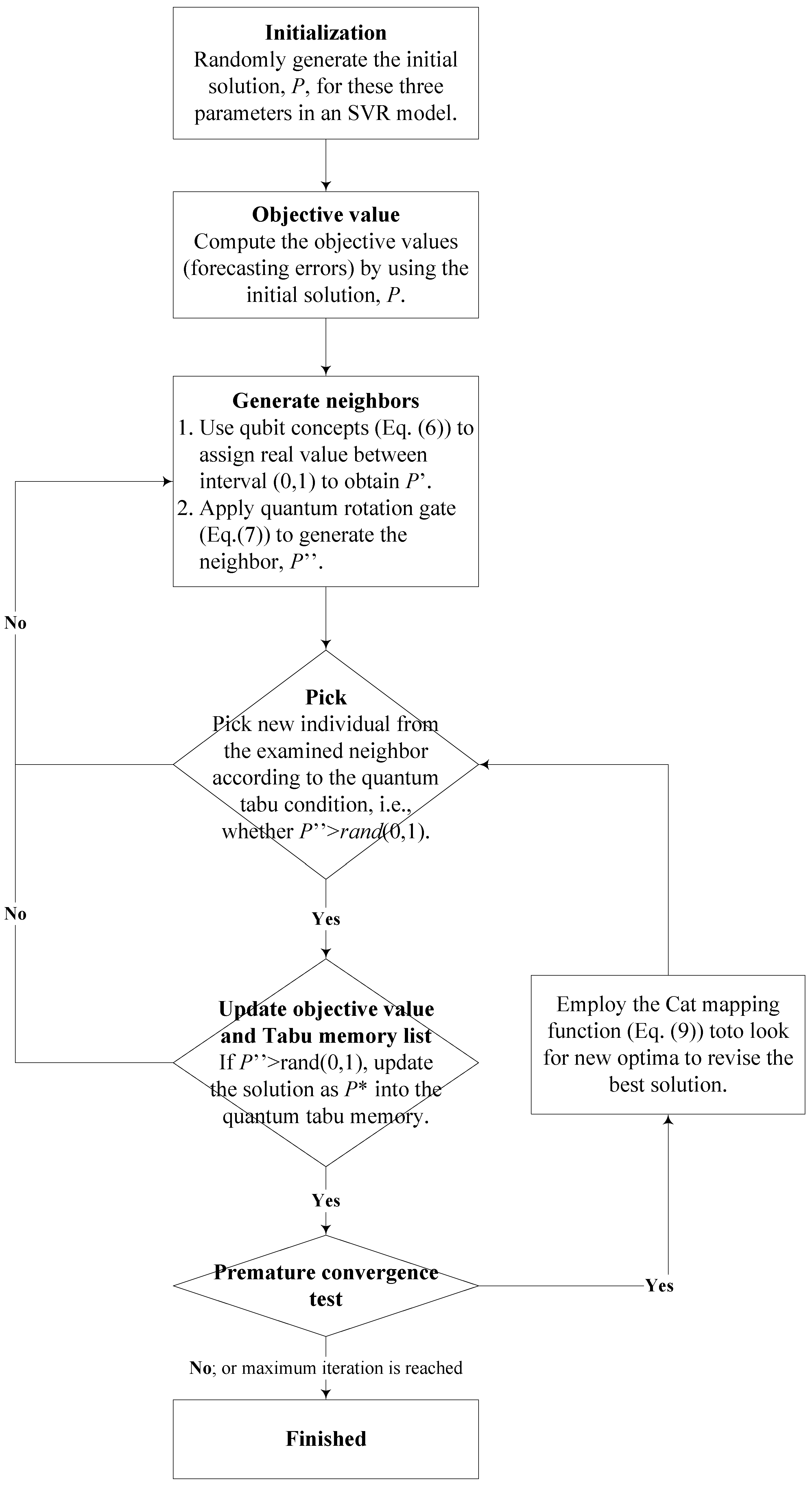
2.2.3. Implementation Steps of Chaotic Quantum Tabu Search (CQTS) Algorithm

The procedure of the hybrid CQTS algorithm with an SVR model is as follows; Figure 1 presents the corresponding flowchart.

Step 1 Initialization. Randomly generate the initial solution, P, that includes the values of three parameters in an SVR model.

Step 2 Objective value. Compute the objective values (forecasting errors) by using the initial solution, P. The mean absolute percentage error (MAPE), given by Equation (10), is used to measure the forecasting errors.

$$MAPE=\frac{1}{N}{\displaystyle \sum _{i=1}^N\left|\frac{y_i-f_i}{y_i}\right|}\times 100\%$$

(10)

where N is the number of forecasting periods; $y_i$ is the actual value in period i; $f_i$ denotes the forecast value in period i.

Step 3 Generate neighbors. Using the qubit concept, Equation (6) sets the initial solution, P, to a real value between interval (0,1) and then obtains P′. Then, use the quantum rotation gate, given by Equation (7), to generate the neighbor, P′′.

Step 4 Pick. Pick a new individual from the examined neighbors based on the quantum tabu condition, which is determined by whether the corresponding value of P′′ exceeds rand(0,1).

Step 5 Update the best solution (objective value) and the tabu memory list. If P′′ > rand(0,1), then update the solution to P* in the quantum tabu memory, v_best. Eventually, the objective value is updated as the current best solution. If the tabu memory is full, then the FIFO rule is applied to eliminate a P* from the list.

Step 6 Premature convergence test. Calculate the mean square error (MSE), given by Equation (11), to evaluate the premature convergence status [69], and set the criteria, δ.

$$MSE=\frac{1}{S}{{\displaystyle \sum _{i=1}^S\left(\frac{f_i-f_{avg}}{f}\right)}}^2$$

(11)

where f_i is the current objective value; f_avg is the mean of all previous objective values, and f is given by Equation (12),

$$f=\max \left\{1,\underset{\forall i\in S}{\max }\left\{\left|f_i-f_{avg}\right|\right\}\right\}$$

(12)

An MSE of less than δ indicates premature convergence. Therefore, the Cat mapping function, Equation (9), is used to find new optima, and the new optimal value is set as the best solution.

Step 7 Stopping criteria. If the stopping threshold (MAPE, which quantifies the forecasting accuracy) or the maximum number of iterations is reached, then training is stopped and the results output; otherwise, the process returns to step 3.

3. Numerical Examples

3.1. Data Set of Numerical Examples

3.1.1. The First Example: Taiwan Regional Load Data

In the first example, Taiwan’s regional electricity load data from a published paper [56,66] are used to establish the proposed SVRCQTS forecasting model. The forecasting performances of this proposed model is compared with that of alternatives. The data set comprises 20 years (from 1981 to 2000) of load values for four regions of Taiwan. This data set is divided into several subsets—a training set (comprising 12 years of load data from 1981 to 1992), a validation set (comprising four years of data from 1993 to 1996), and a testing set (comprising four years of data from 1997 to 2000). The forecasting performances are measured using MAPE (Equation (10)).

In the training stage, the rolling forecasting procedure, proposed by Hong [56], is utilized to help CQTS algorithm determining appropriate parameter values of an SVR model in the training stage, and eventually, receive more satisfied results. For details, the training set is further divided into two subsets, namely the fed-in (for example, n load data) and the fed-out (12 − n load data), respectively. Firstly, the preceding n load data are used to minimize the training error by the structural risk principle; then, receive one-step-ahead (in-sample) forecasting load, i.e., the (n + 1)th forecasting load. Secondly, the next n load data, i.e., from 2nd to (n + 1)th data, are set as the new fed-in and similarly used to minimize the training error again to receive the second one-step-ahead (in-sample) forecasting load, named as the (n + 2)th forecasting load. Repeat this procedure until the 12nd (in-sample) forecasting load is obtained with the training error. The training error can be obtained during each iteration, these parameters would be decided by QTS algorithm, and the validation error would be also calculated in the meanwhile. Only with the smallest validation and testing errors will the adjusted parameter combination be selected as the most appropriate parameter combination. The testing data set is only used for examining the forecasting accuracy level. Eventually, the four-year forecasting electricity load demands in each region are forecasted by the SVRCQTS model. The complete process is illustrated in Figure 2.

3.1.2. The Second Example: Taiwan Annual Load Data

In the second example, Taiwan’s annual electricity load data from a published paper are used [56,66]. The data set is composed of 59 years of load data (from 1945 to 2003), which are divided into three subsets—a training set (40 years of load data from 1945 to 1984), a validation set (10 ten of load data from 1985 to 1994), and a testing set (nine years of load data from 1995 to 2003). The relevant modeling procedures are as in the first example.

3.1.3. The Third Example: 2014 Global Energy Forecasting Competition (GEFCOM 2014) Load Data

The third example involves the 744 h of load data from the 2014 Global Energy Forecasting Competition [70] (from 00:00 1 December 2011 to 00:00 1 January 2012). The data set is divided into three subsets—a training set (552 h of load data from 01:00 1 December 2011 to 00:00 24 December 2011), a validation set (96 h of load data from 01:00 24 December 2011 to 00:00 28 December 2011), and testing set (96 h of load data from 01:00 28 December 2011 to 00:00 1 January 2012). The relevant modeling procedures are as in the preceding two examples.

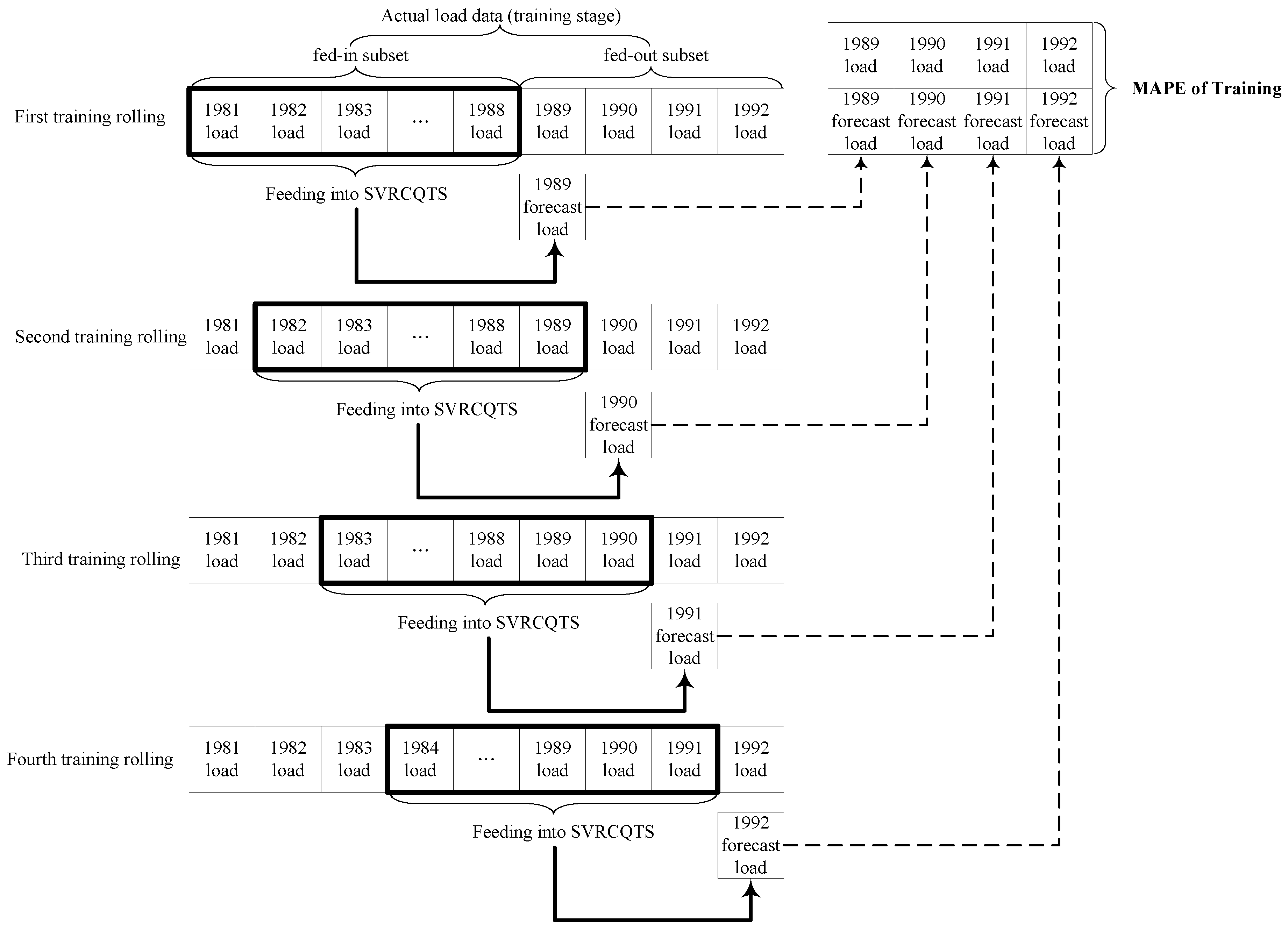
3.2. The SVRCQTS Load Forecasting Model

3.2.1. Parameters Setting in CQTS Algorithm

For some controlling parameters settings during modeling process, such as the total number of iteration is all fixed as 10,000; $\mathsf{\sigma }\in \left[0,15\right]$, $\mathsf{\epsilon }\in \left[0,100\right]$ in all examples, $C\in \left[0,\mathrm{20,000}\right]$ in Example 1, $C\in \left[0,3\times {10}^{10}\right]$ in Examples 2 and 3; δ is all set to 0.001.

3.2.2. Forecasting Results and Analysis for Example 1

In Example 1, the combination of parameters of the most appropriate model are evaluated using the QTS algorithm and the CQTS algorithm for each region, and almost has the smallest testing MAPE value.

Table 1. Parameters determination of SVRCQTS and SVRQTS models (example 1). SVRCQTS: support vector regression chaotic quantum tabu search; SVRQTS: support vector regression quantum Tabu search.

Regions	SVRCQTS Parameters			MAPE of Testing (%)
	σ	C	ε
Northern	10.0000	$0.8000\times {10}^{10}$	0.7200	1.0870
Central	6.0000	$1.6000\times {10}^{10}$	0.5500	1.2650
Southern	8.0000	$1.4000\times {10}^{10}$	0.6500	1.1720
Eastern	8.0000	$0.8000\times {10}^{10}$	0.4300	1.5430
Regions	SVRQTS Parameters			MAPE of Testing (%)
	σ	C	ε
Northern	4.0000	$0.8000\times {10}^{10}$	0.2500	1.3260
Central	12.0000	$1.0000\times {10}^{10}$	0.2800	1.6870
Southern	10.0000	$0.8000\times {10}^{10}$	0.7200	1.3670
Eastern	8.0000	$1.4000\times {10}^{10}$	0.4200	1.9720

presents these well-determined parameters for each region.

Table 2. Forecasting results (and absolute errors) of SVRCQTS, SVRQTS, and other models (example 1) (unit: 10⁶ Wh).

Year	Northern Region
	SVRCQTS	SVRQTS	SVRCQPSO	SVRQPSO	SVRCPSO	SVRPSO
1997	11,123 (101)	11,101 (121)	11,339 (117)	11,046 (176)	11,232 (10)	11,245 (23)
1998	11,491 (151)	11,458 (184)	11,779 (137)	11,787 (145)	11,628 (14)	11,621 (21)
1999	12,123 (142)	12,154 (173)	11,832 (149)	12,144 (163)	12,016 (35)	12,023 (42)
2000	13,052 (128)	13,080 (156)	12,798 (126)	12,772 (152)	12,306 (618)	12,306 (618)
MAPE (%)	1.0870	1.3260	1.1070	1.3370	1.3187	1.3786
Year	Central Region
	SVRCQTS	SVRQTS	SVRCQPSO	SVRQPSO	SVRCPSO	SVRPSO
1997	5009 (52)	5132 (71)	4987 (74)	5140 (79)	5066 (5)	5085 (24)
1998	5167 (79)	5142 (104)	5317 (71)	5342 (96)	5168 (78)	5141 (105)
1999	5301 (68)	5318 (85)	5172 (61)	5130 (103)	5232 (1)	5236 (3)
2000	5702 (69)	5732 (99)	5569 (64)	5554 (79)	5313 (320)	5343 (290)
MAPE (%)	1.2650	1.6870	1.2840	1.6890	1.8100	1.9173
Year	Southern Region
	SVRCQTS	SVRQTS	SVRCQPSO	SVRQPSO	SVRCPSO	SVRPSO
1997	6268 (68)	6436 (100)	6262 (74)	6265 (71)	6297 (39)	6272 (64)
1998	6398 (80)	6245 (73)	6401 (83)	6418 (100)	6311 (7)	6314 (4)
1999	6343 (84)	6338 (79)	6179 (80)	6178 (81)	6324 (65)	6327 (68)
2000	6735 (69)	6704 (100)	6738 (66)	6901 (97)	6516 (288)	6519 (285)
MAPE (%)	1.1720	1.3670	1.1840	1.3590	1.4937	1.5899
Year	Eastern Region
	SVRCQTS	SVRQTS	SVRCQPSO	SVRQPSO	SVRCPSO	SVRPSO
1997	362 (4)	364 (6)	353 (5)	350 (8)	370 (12)	367 (9)
1998	390 (7)	388 (9)	404 (7)	390 (7)	376 (21)	374 (23)
1999	395 (6)	394 (7)	394 (7)	410 (9)	411 (10)	409 (8)
2000	427 (7)	429 (9)	414 (6)	413 (7)	418 (2)	415 (5)
MAPE (%)	1.5430	1.9720	1.5940	1.9830	2.1860	2.3094

Note: *: The values in the parentheses are the absolute error, which is defined as: $\left|y_i-f_i\right|$, where $y_i$ is the actual value in period i; $f_i$ denotes is the forecast value in period i. SVRCQPSO: support vector regression chaotic quantum particle swarm optimization; SVRQPSO: support vector regression quantum particle swarm optimization ; SVRCPSO: support vector regression chaotic particle swarm optimization; SVRPSO: support vector regression particle swarm optimization.

presents the forecasting accuracy index (MAPE) and electricity load values of each region that are forecast, under the same conditions, using alternative models, which were include SVRCQTS, SVRQTS, SVR with chaotic particle swarm optimization (SVRCQPSO), SVR with quantum PSO (SVRQPSO), and SVR with PSO (SVRPSO) models. Clearly, according to Table 2, the SVRCQTS model is superior to the other SVR-based models. Applying quantum computing mechanics to the TS algorithm is a feasible means of improving the satisfied, and thus improving the forecasting accuracy of the SVR model. The Cat mapping function has a critical role in finding an improved solution when the QTS algorithm becomes trapped in local optima or requires a long time to solve the problem of interest). For example, for the central region, the QTS algorithm is utilized to find the best solution, (σ, C, ε) = (12.0000, 1.0000 × 1010, 0.2800), with a forecasting error, MAPE, of 1.6870%. The solution can be further improved by using the CQTS algorithm with (σ, C, ε) = (6.0000, 1.6000 × 1010, 0.5500), which has a smaller forecasting accuracy of 1.2650%. For other regions, the QTS algorithm yields an increased forecasting performance to 1.3260% (northern region), 1.3670% (southern region) and 1.9720% (eastern region). All of these models can also be further improved to increase the accuracy of the forecasting results by using the Cat mapping function (the CQTS algorithm), yielding a forecasting accuracy of 1.087% for the northern region, 1.1720% for the southern region, and 1.5430% for the eastern region.

To verify that the proposed SVRCQTS and SVRQTS models offers an improved forecasting accuracy, the Wilcoxon signed-rank test, recommended by Diebold and Mariano [71], is used. In this work, the Wilcoxon signed-rank test is performed with two significance levels, α = 0.025 and α = 0.005, by one-tail-tests.

Table 3. Wilcoxon signed-rank test (example 1).

Compared Models		Wilcoxon Signed-Rank Test
		α = 0.025; W = 0	α = 0.005; W = 0	p-Value
Northern region	SVRCQTS vs. SVRPSO	0 a	0 a	N/A
	SVRCQTS vs. SVRCPSO	0 a	0 a	N/A
	SVRCQTS vs. SVRQPSO	0 a	0 a	N/A
	SVRCQTS vs. SVRCQPSO	0 a	0 a	N/A
	SVRCQTS vs. SVRQTS	1	1	N/A
Central region	SVRCQTS vs. SVRPSO	0 a	0 a	N/A
	SVRCQTS vs. SVRCPSO	0 a	0 a	N/A
	SVRCQTS vs. SVRQPSO	0 a	0 a	N/A
	SVRCQTS vs. SVRCQPSO	1	1	N/A
	SVRCQTS vs. SVRQTS	0 a	0 a	N/A
Southern region	SVRCQTS vs. SVRPSO	0 a	0 a	N/A
	SVRCQTS vs. SVRCPSO	0 a	0 a	N/A
	SVRCQTS vs. SVRQPSO	0 a	0 a	N/A
	SVRCQTS vs. SVRCQPSO	1	1	N/A
	SVRCQTS vs. SVRQTS	0 a	0 a	N/A
Eastern region	SVRCQTS vs. SVRPSO	0 a	0 a	N/A
	SVRCQTS vs. SVRCPSO	0 a	0 a	N/A
	SVRCQTS vs. SVRQPSO	0 a	0 a	N/A
	SVRCQTS vs. SVRCQPSO	1	1	N/A
	SVRCQTS vs. SVRQTS	0 a	0 a	N/A

Note: ^a denotes that the SVRCQTS model significantly outperforms other alternative models.

presents the test results, which reveal that the SVRCQTS model significantly outperforms other models for the northern and eastern regions in terms of MAPE.

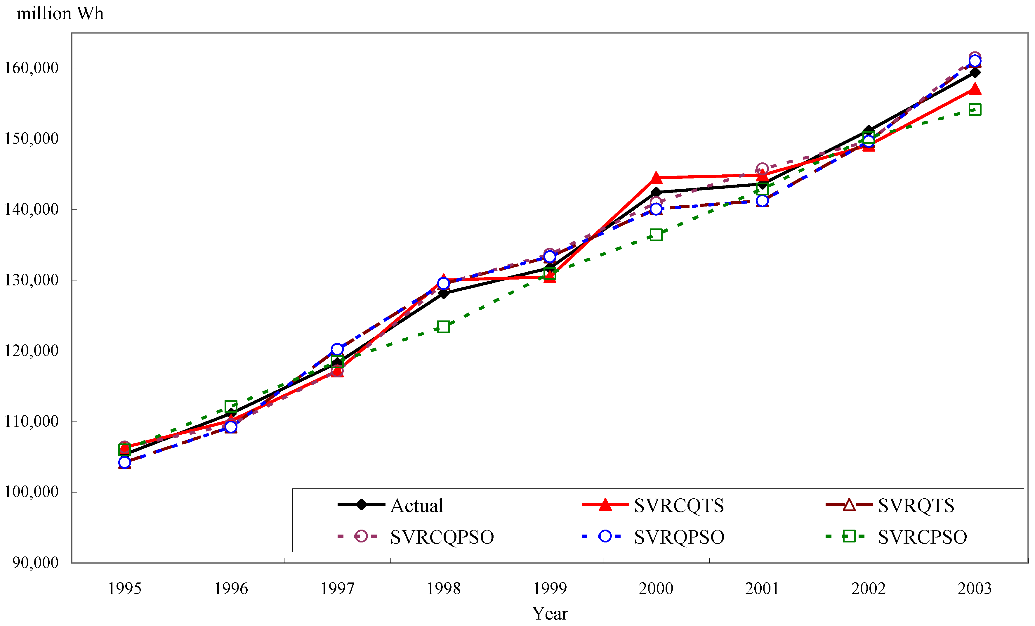
3.2.3. Forecasting Results and Analysis for Example 2

In Example 2, the processing steps are those in the preceding example. The parameters in an SVR model are computed using the QTS algorithm and the CQTS algorithm. The finalized models exhibit the best forecasting performance with the smallest MAPE values.

Table 4. Parameters determination of SVRCQTS and SVRQTS models (Example 2). PSO: particle swarm optimization; CPSO: chaotic particle swarm optimization; QPSO: quantum particle swarm optimization; CQPSO: chaotic quantum particle swarm optimization.

Optimization Algorithms	Parameters			MAPE of Testing (%)
	σ	C	ε
PSO algorithm [56]	0.2293	$1.7557\times {10}^{11}$	10.175	3.1429
CPSO algorithm [56]	0.2380	$2.3365\times {10}^{11}$	39.296	1.6134
QPSO algorithm [66]	12.0000	$0.8000\times {10}^{11}$	0.380	1.3460
CQPSO algorithm [66]	10.0000	$1.5000\times {10}^{11}$	0.560	1.1850
QTS algorithm	5.0000	$1.3000\times {10}^{11}$	0.630	1.3210
CQTS algorithm	6.0000	$1.8000\times {10}^{11}$	0.340	1.1540

presents the well determined parameters for annual electricity load data. To compare with other benchmarking algorithms, Table 4 presents all results from relevant papers on SVR-based modeling, such as those of Hong [56], who proposed the SVRCPSO and SVR with PSO (SVRPSO) models and Huang [66], who proposed the SVRCQPSO and SVRQPSO models.

Table 5. Forecasting results (and absolute errors) of SVRCQTS, SVRQTS, and other models (unit: 10⁶ Wh).

Years	SVRCQTS	SVRQTS	SVRCQPSO	SVRQPSO	SVRCPSO	SVRPSO
1995	106,353 (985)	104,241 (1127)	106,379 (1011)	104,219 (1149)	105,960 (592)	102,770 (2598)
1996	110,127 (1013)	109,246 (1894)	109,573 (1567)	109,210 (1930)	112,120 (980)	109,800 (1340)
1997	117,180 (1119)	120,174 (1875)	117,149 (1150)	120,210 (1911)	118,450 (151)	115,570 (2729)
1998	130,023 (1893)	129,501 (1371)	129,466 (1336)	129,527 (1397)	123,400 (4730)	120,650 (7480)
1999	130,464 (1262)	133,275 (1549)	133,646 (1920)	133,304 (1578)	130,940 (786)	128,240 (3486)
2000	144,500 (2087)	140,099 (2314)	140,945 (1468)	140,055 (2358)	136,420 (5993)	137,250 (5163)
2001	144,884 (1260)	141,271 (2353)	145,734 (2110)	141,227 (2397)	142,910 (714)	140,230 (3394)
2002	149,099 (2094)	149,675 (1518)	149,652 (1541)	149,646 (1547)	150,210 (983)	151,150 (43)
2003	157,099 (2281)	161,001 (1621)	161,458 (2078)	161,032 (1652)	154,130 (5250)	146,940 (12,440)
MAPE (%)	1.1540	1.3210	1.1850	1.3460	1.6134	3.1429

Note: *: the value in the parentheses is the absolute error which is defined as: $\left|y_i-f_i\right|$, where $y_i$ is the actual value in period i; $f_i$ denotes is the forecast value in period i.

presents the MAPE values and forecasting results obtained using the alternative forecasting models. The SVRCQTS model outperforms the other models, indicating quantum computing is an ideal approach to improve the performance of any SVR-based model, and that the Cat mapping function is very effective for solving the problem of premature convergence and the fact that it is time-saving. Clearly, the QTS algorithm yields (σ, C, ε) = (5.0000, 1.3000 × 10¹¹, 0.630) with a MAPE of 1.3210%, whereas the CQTS algorithm provides a better solution, (σ, C, ε) = (6.0000, 1.8000 × 10¹¹, 0.340) with a MAPE of 1.1540%. Figure 3 presents the real values and the forecast values obtained using the various models.

To ensure the significance of the proposed SVRCQTS model in Example 2, the Wilcoxon signed-rank test is again considered performed.

Table 6. Wilcoxon signed-rank test (example 2).

Compared Models	Wilcoxon Signed-Rank Test
	α = 0.025; W = 5	α = 0.005; W = 8	p-Value
SVRCQTS vs. SVRPSO	2 a	2 a	N/A
SVRCQTS vs. SVRCPSO	3 a	3 a	N/A
SVRCQTS vs. SVRQPSO	4 a	4 a	N/A
SVRCQTS vs. SVRCQPSO	4 a	4 a	N/A
SVRCQTS vs. SVRQTS	4 a	4 a	N/A

Note: ^a denotes that the SVRCQTS model significantly outperforms other alternative models.

shows that the SVRCQTS model passes the test and significantly improves on other alternatives.

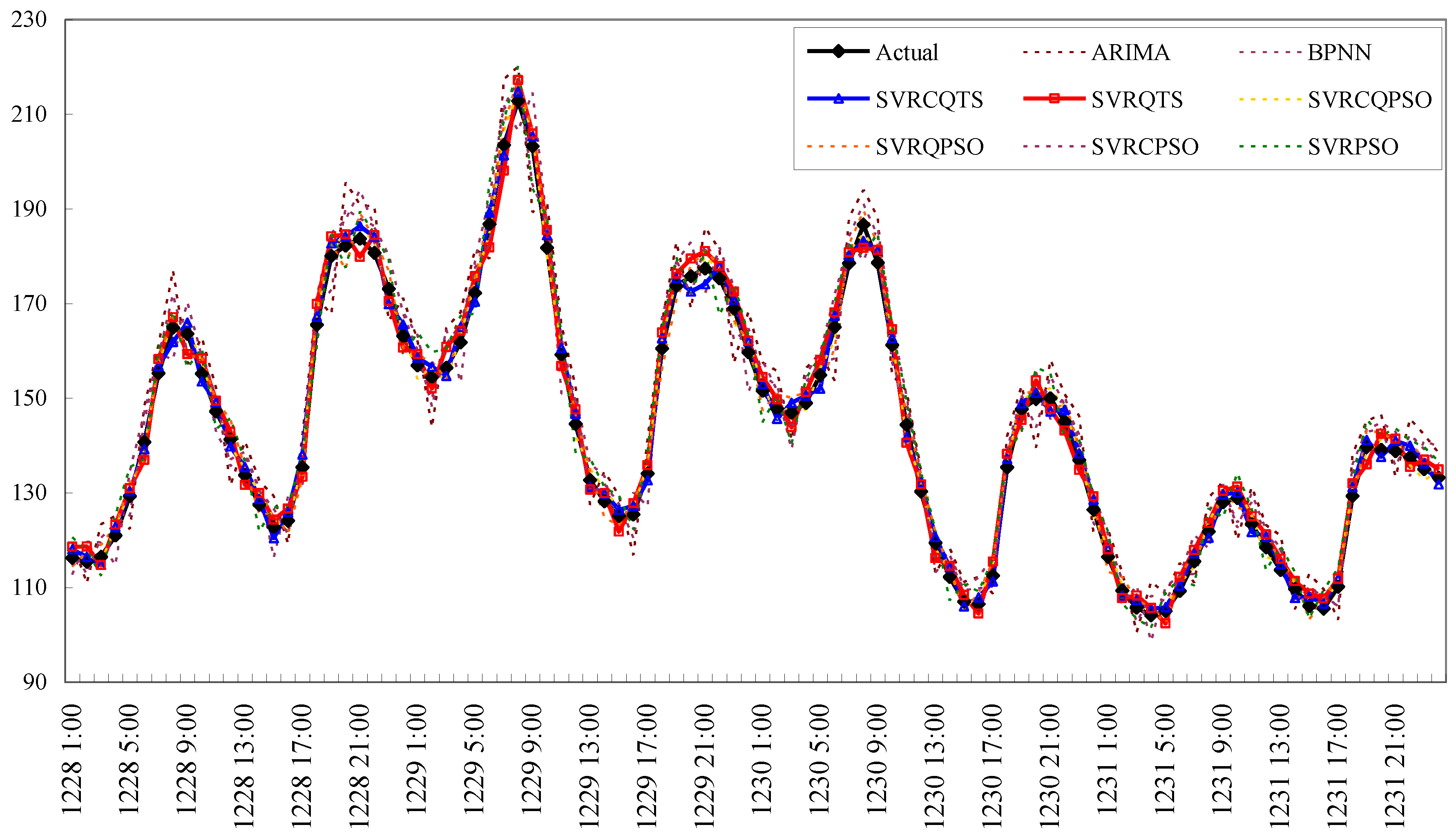
3.2.4. Forecasting Results and Analysis for Example 3

In Example 3, the modeling processes are the same as in the preceding two examples. The parameters in the SVR model are calculated using the QTS algorithm and the CQTS algorithm.

Table 7. Parameters determination of SVRCQTS, SVRQTS, and other models (Example 3).

Optimization Algorithms	Parameters			MAPE of Testing (%)
	σ	C	ε
PSO algorithm [66]	7.000	34.000	0.9400	3.1500
CPSO algorithm [66]	22.000	19.000	0.6900	2.8600
QPSO algorithm [66]	9.000	42.000	0.1800	1.9600
CQPSO algorithm [66]	19.000	35.000	0.8200	1.2900
QTS algorithm	25.000	67.000	0.0900	1.8900
CQTS algorithm	12.000	26.000	0.3200	1.3200

presents the details of the determined models and the alternatives models for the GEFCOM 2014 data set. Huang [66] used the GEFCOM 2014 load data to forecast the electric load, therefore, the models of Huang [66] are included in this paper as the alternative models.

The alternative models of Huang [66]—ARIMA(0,1,1), back propagation neural networks (BPNN), SVRPSO, SVRCPSO, SVRQPSO, SVRCQPSO, and SVRQTS models—are compared herein under fixed conditions. Figure 4 displays the real values and the forecast results obtained using all compared models, and demonstrates that the SVRCQTS model outperforms the SVRQTS and SVRQPSO models. It also reveals that applying quantum computing mechanics to the TS algorithm improves the forecasting accuracy level for any SVR-based models. The SVRCQTS model has a smaller MAPE value than the SVRQTS model.

Finally,

Table 8. Wilcoxon signed-rank test (Example 3).

Compared Models	Wilcoxon Signed-Rank Test
	α = 0.025; W = 2328	α = 0.05; W = 2328	p-Value
SVRCQTS vs. ARIMA	1621 a	1621 a	0.00988
SVRCQTS vs. BPNN	1600 a	1600 a	0.00782
SVRCQTS vs. SVRPSO	2148	2148 a	0.04318
SVRCQTS vs. SVRCPSO	2163	2163 a	0.04763
SVRCQTS vs. SVRQPSO	1568 a	1568 a	0.00544
SVRCQTS vs. SVRCQPSO	1344 a	1344 a	0.00032
SVRCQTS vs. SVRQTS	1741	1741 a	0.03156

Note: ^a denotes that the SVRCQTS model significantly outperforms other alternative models.

presents the results of the Wilcoxon signed-rank test. It indicates that the proposed SVRCQTS model almost receives statistical significance in forecasting performances under the significant level, α = 0.05. Therefore, the proposed SVRCQTS model significantly outperforms other alternatives in terms of α = 0.05.

4. Conclusions

This work proposes a hybrid model that incorporates an SVR-based model, the chaotic cat mapping function, and the QTS algorithm for forecasting electricity load demand. Experimental results reveal that the proposed model exhibits significantly better forecasting performance than other SVR-based forecasting models. In this paper, quantum mechanics is utilized to improve the intensification and diversification of the simple TS algorithm, and thereby to improve its forecasting accuracy. Chaotic cat mapping is also used to help prevent the QTS algorithm from becoming trapped in local optima in the modeling processes. This work marks a favorable beginning of the hybridization of quantum computing mechanics and the chaotic mechanism to expand the search space, which is typically limited by Newtonian dynamics.

References

1. Bunn, D.W.; Farmer, E.D. Comparative models for electrical load forecasting. Int. J. Forecast. 1986, 2, 241–242. [Google Scholar]
2. Fan, S.; Chen, L. Short-term load forecasting based on an adaptive hybrid method. IEEE Trans. Power Syst. 2006, 21, 392–401. [Google Scholar] [CrossRef]
3. Morimoto, R.; Hope, C. The impact of electricity supply on economic growth in Sri Lanka. Energy Econ. 2004, 26, 77–85. [Google Scholar] [CrossRef]
4. Zhao, W.; Wang, J.; Lu, H. Combining forecasts of electricity consumption in China with time-varying weights updated by a high-order Markov chain model. Omega 2014, 45, 80–91. [Google Scholar] [CrossRef]
5. Wang, J.; Wang, J.; Li, Y.; Zhu, S.; Zhao, J. Techniques of applying wavelet de-noising into a combined model for short-term load forecasting. Int. J. Electr. Power Energy Syst. 2014, 62, 816–824. [Google Scholar] [CrossRef]
6. Hussain, A.; Rahman, M.; Memon, J.A. Forecasting electricity consumption in Pakistan: The way forward. Energy Policy 2016, 90, 73–80. [Google Scholar] [CrossRef]
7. Maçaira, P.M.; Souza, R.C.; Oliveira, F.L.C. Modelling and forecasting the residential electricity consumption in Brazil with pegels exponential smoothing techniques. Procedia Comput. Sci. 2015, 55, 328–335. [Google Scholar] [CrossRef]
8. Al-Hamadi, H.M.; Soliman, S.A. Short-term electric load forecasting based on Kalman filtering algorithm with moving window weather and load model. Electr. Power Syst. Res. 2004, 68, 47–59. [Google Scholar] [CrossRef]
9. Zheng, T.; Girgis, A.A.; Makram, E.B. A hybrid wavelet-Kalman filter method for load forecasting. Electr. Power Syst. Res. 2000, 54, 11–17. [Google Scholar] [CrossRef]
10. Blood, E.A.; Krogh, B.H.; Ilic, M.D. Electric power system static state estimation through Kalman filtering and load forecasting. In Proceedings of the Power and Energy Society General Meeting—Conversion and Delivery of Electrical Energy in the 21st Century, Pittsburgh, PA, USA, 20–24 July 2008.
11. Hippert, H.S.; Taylor, J.W. An evaluation of Bayesian techniques for controlling model complexity and selecting inputs in a neural network for short-term load forecasting. Neural Netw. 2010, 23, 386–395. [Google Scholar] [CrossRef] [PubMed]
12. Zhang, W.; Yang, J. Forecasting natural gas consumption in China by Bayesian model averaging. Energy Rep. 2015, 1, 216–220. [Google Scholar] [CrossRef]
13. Chai, J.; Guo, J.E.; Lu, H. Forecasting energy demand of China using Bayesian combination model. China Popul. Resour. Environ. 2008, 18, 50–55. [Google Scholar]
14. Vu, D.H.; Muttaqi, K.M.; Agalgaonkar, A.P. A variance inflation factor and backward elimination based robust regression model for forecasting monthly electricity demand using climatic variables. Appl. Energy 2015, 140, 385–394. [Google Scholar] [CrossRef]
15. Dudek, G. Pattern-based local linear regression models for short-term load forecasting. Electr. Power Syst. Res. 2016, 130, 139–147. [Google Scholar] [CrossRef]
16. Wu, J.; Wang, J.; Lu, H.; Dong, Y.; Lu, X. Short term load forecasting technique based on the seasonal exponential adjustment method and the regression model. Energy Convers. Manag. 2013, 70, 1–9. [Google Scholar] [CrossRef]
17. Hernández, L.; Baladrón, C.; Aguiar, J.M.; Carro, B.; Sánchez-Esguevillas, A.; Lloret, J. Artificial neural networks for short-term load forecasting in microgrids environment. Energy 2014, 75, 252–264. [Google Scholar] [CrossRef]
18. Ertugrul, Ö.F. Forecasting electricity load by a novel recurrent extreme learning machines approach. Int. J. Electr. Power Energy Syst. 2016, 78, 429–435. [Google Scholar] [CrossRef]
19. Quan, H.; Srinivasan, D.; Khosravi, A. Uncertainty handling using neural network-based prediction intervals for electrical load forecasting. Energy 2014, 73, 916–925. [Google Scholar] [CrossRef]
20. Li, P.; Li, Y.; Xiong, Q.; Chai, Y.; Zhang, Y. Application of a hybrid quantized Elman neural network in short-term load forecasting. Int. J. Electr. Power Energy Syst. 2014, 55, 749–759. [Google Scholar] [CrossRef]
21. Sousa, J.C.; Neves, L.P.; Jorge, H.M. Assessing the relevance of load profiling information in electrical load forecasting based on neural network models. Int. J. Electr. Power Energy Syst. 2012, 40, 85–93. [Google Scholar] [CrossRef]
22. Lahouar, A.; Slama, J.B.H. Day-ahead load forecast using random forest and expert input selection. Energy Convers. Manag. 2015, 103, 1040–1051. [Google Scholar] [CrossRef]
23. Bennett, C.J.; Stewart, R.A.; Lu, J.W. Forecasting low voltage distribution network demand profiles using a pattern recognition based expert system. Energy 2014, 67, 200–212. [Google Scholar] [CrossRef]
24. Santana, Á.L.; Conde, G.B.; Rego, L.P.; Rocha, C.A.; Cardoso, D.L.; Costa, J.C.W.; Bezerra, U.H.; Francês, C.R.L. PREDICT—Decision support system for load forecasting and inference: A new undertaking for Brazilian power suppliers. Int. J. Electr. Power Energy Syst. 2012, 38, 33–45. [Google Scholar] [CrossRef]
25. Efendi, R.; Ismail, Z.; Deris, M.M. A new linguistic out-sample approach of fuzzy time series for daily forecasting of Malaysian electricity load demand. Appl. Soft Comput. 2015, 28, 422–430. [Google Scholar] [CrossRef]
26. Hooshmand, R.-A.; Amooshahi, H.; Parastegari, M. A hybrid intelligent algorithm based short-term load forecasting approach. Int. J. Electr. Power Energy Syst. 2013, 45, 313–324. [Google Scholar] [CrossRef]
27. Akdemir, B.; Çetinkaya, N. Long-term load forecasting based on adaptive neural fuzzy inference system using real energy data. Energy Procedia 2012, 14, 794–799. [Google Scholar] [CrossRef]
28. Chaturvedi, D.K.; Sinha, A.P.; Malik, O.P. Short term load forecast using fuzzy logic and wavelet transform integrated generalized neural network. Int. J. Electr. Power Energy Syst. 2015, 67, 230–237. [Google Scholar] [CrossRef]
29. Liao, G.-C. Hybrid Improved Differential Evolution and Wavelet Neural Network with load forecasting problem of air conditioning. Int. J. Electr. Power Energy Syst. 2014, 61, 673–682. [Google Scholar] [CrossRef]
30. Zhai, M.-Y. A new method for short-term load forecasting based on fractal interpretation and wavelet analysis. Int. J. Electr. Power Energy Syst. 2015, 69, 241–245. [Google Scholar] [CrossRef]
31. Zeng, X.; Shu, L.; Huang, G.; Jiang, J. Triangular fuzzy series forecasting based on grey model and neural network. Appl. Math. Model. 2016, 40, 1717–1727. [Google Scholar] [CrossRef]
32. Efendigil, T.; Önüt, S.; Kahraman, C. A decision support system for demand forecasting with artificial neural networks and neuro-fuzzy models: A comparative analysis. Expert Syst. Appl. 2009, 36, 6697–6707. [Google Scholar] [CrossRef]
33. Coelho, V.N.; Coelho, I.M.; Coelho, B.N.; Reis, A.J.R.; Enayatifar, R.; Souza, M.J.F.; Guimarães, F.G. A self-adaptive evolutionary fuzzy model for load forecasting problems on smart grid environment. Appl. Energy 2016, 169, 567–584. [Google Scholar] [CrossRef]
34. Khashei, M.; Mehdi Bijari, M. A novel hybridization of artificial neural networks and ARIMA models for time series forecasting. Appl. Soft Comput. 2011, 11, 2664–2675. [Google Scholar] [CrossRef]
35. Ghanbari, A.; Kazemi, S.M.R.; Mehmanpazir, F.; Nakhostin, M.M. A Cooperative Ant Colony Optimization-Genetic Algorithm approach for construction of energy demand forecasting knowledge-based expert systems. Knowl.-Based Syst. 2013, 39, 194–206. [Google Scholar] [CrossRef]
36. Bahrami, S.; Hooshmand, R.-A.; Parastegari, M. Short term electric load forecasting by wavelet transform and grey model improved by PSO (particle swarm optimization) algorithm. Energy 2014, 72, 434–442. [Google Scholar] [CrossRef]
37. Suykens, J.A.K.; Vandewalle, J.; De Moor, B. Optimal control by least squares support vector machines. Neural Netw. 2001, 14, 23–35. [Google Scholar] [CrossRef]
38. Aras, S.; Kocakoç, İ.D. A new model selection strategy in time series forecasting with artificial neural networks: IHTS. Neurocomputing 2016, 174, 974–987. [Google Scholar] [CrossRef]
39. Kendal, S.L.; Creen, M. An Introduction to Knowledge Engineering; Springer: London, UK, 2007. [Google Scholar]
40. Cherroun, L.; Hadroug, N.; Boumehraz, M. Hybrid approach based on ANFIS models for intelligent fault diagnosis in industrial actuator. J. Control Electr. Eng. 2013, 3, 17–22. [Google Scholar]
41. Hahn, H.; Meyer-Nieberg, S.; Pickl, S. Electric load forecasting methods: Tools for decision making. Eur. J. Oper. Res. 2009, 199, 902–907. [Google Scholar] [CrossRef]
42. Drucker, H.; Burges, C.C.J.; Kaufman, L.; Smola, A.; Vapnik, V. Support vector regression machines. Adv. Neural Inf. Process Syst. 1997, 9, 155–161. [Google Scholar]
43. Tay, F.E.H.; Cao, L.J. Modified support vector machines in financial time series forecasting. Neurocomputing 2002, 48, 847–861. [Google Scholar] [CrossRef]
44. Hong, W.C. Electric load forecasting by seasonal recurrent SVR (support vector regression) with chaotic artificial bee colony algorithm. Energy 2011, 36, 5568–5578. [Google Scholar] [CrossRef]
45. Chen, Y.H.; Hong, W.C.; Shen, W.; Huang, N.N. Electric load forecasting based on LSSVM with fuzzy time series and global harmony search algorithm. Energies 2016, 9, 70. [Google Scholar] [CrossRef]
46. Fan, G.; Peng, L.-L.; Hong, W.-C.; Sun, F. Electric load forecasting by the SVR model with differential empirical mode decomposition and auto regression. Neurocomputing 2016, 173, 958–970. [Google Scholar] [CrossRef]
47. Geng, J.; Huang, M.L.; Li, M.W.; Hong, W.C. Hybridization of seasonal chaotic cloud simulated annealing algorithm in a SVR-based load forecasting model. Neurocomputing 2015, 151, 1362–1373. [Google Scholar] [CrossRef]
48. Ju, F.Y.; Hong, W.C. Application of seasonal SVR with chaotic gravitational search algorithm in electricity forecasting. Appl. Math. Model. 2013, 37, 9643–9651. [Google Scholar] [CrossRef]
49. Fan, G.; Wang, H.; Qing, S.; Hong, W.C.; Li, H.J. Support vector regression model based on empirical mode decomposition and auto regression for electric load forecasting. Energies 2013, 6, 1887–1901. [Google Scholar] [CrossRef]
50. Hong, W.C.; Dong, Y.; Zhang, W.Y.; Chen, L.Y.; Panigrahi, B.K. Cyclic electric load forecasting by seasonal SVR with chaotic genetic algorithm. Int. J. Electr. Power Energy Syst. 2013, 44, 604–614. [Google Scholar] [CrossRef]
51. Zhang, W.Y.; Hong, W.C.; Dong, Y.; Tsai, G.; Sung, J.T.; Fan, G. Application of SVR with chaotic GASA algorithm in cyclic electric load forecasting. Energy 2012, 45, 850–858. [Google Scholar] [CrossRef]
52. Hong, W.C.; Dong, Y.; Lai, C.Y.; Chen, L.Y.; Wei, S.Y. SVR with hybrid chaotic immune algorithm for seasonal load demand forecasting. Energies 2011, 4, 960–977. [Google Scholar] [CrossRef]
53. Hong, W.C. Application of chaotic ant swarm optimization in electric load forecasting. Energy Policy 2010, 38, 5830–5839. [Google Scholar] [CrossRef]
54. Hong, W.C. Hybrid evolutionary algorithms in a SVR-based electric load forecasting model. Int. J. Electr. Power Energy Syst. 2009, 31, 409–417. [Google Scholar] [CrossRef]
55. Hong, W.C. Electric load forecasting by support vector model. Appl. Math. Model. 2009, 33, 2444–2454. [Google Scholar] [CrossRef]
56. Hong, W.C. Chaotic particle swarm optimization algorithm in a support vector regression electric load forecasting model. Energy Convers. Manag. 2009, 50, 105–117. [Google Scholar] [CrossRef]
57. Glover, F. Tabu search, part I. ORSA J. Comput. 1989, 1, 190–206. [Google Scholar] [CrossRef]
58. Glover, F. Tabu search, part II. ORSA J. Comput. 1990, 2, 4–32. [Google Scholar] [CrossRef]
59. Zeng, Z.; Yu, X.; He, K.; Huang, W.; Fu, Z. Iterated tabu search and variable neighborhood descent for packing unequal circles into a circular container. Eur. J. Oper. Res. 2016, 250, 615–627. [Google Scholar] [CrossRef]
60. Lai, D.S.W.; Demirag, O.C.; Leung, J.M.Y. A tabu search heuristic for the heterogeneous vehicle routing problem on a multigraph. Trans. Res. E Logist. Trans. Rev. 2016, 86, 32–52. [Google Scholar] [CrossRef]
61. Wu, Q.; Wang, Y.; Lü, Z. A tabu search based hybrid evolutionary algorithm for the max-cut problem. Appl. Soft Comput. 2015, 34, 827–837. [Google Scholar] [CrossRef]
62. Kvasnicka, V.; Pospichal, J. Fast evaluation of chemical distance by tabu search algorithm. J. Chem. Inf. Comput. Sci. 1994, 34, 1109–1112. [Google Scholar] [CrossRef]
63. Amaral, P.; Pais, T.C. Compromise Ratio with weighting functions in a Tabu Search multi-criteria approach to examination timetabling. Comput. Oper. Res. 2016, 72, 160–174. [Google Scholar] [CrossRef]
64. Shen, Q.; Shi, W.-M.; Kong, W. Modified tabu search approach for variable selection in quantitative structure–activity relationship studies of toxicity of aromatic compounds. Artif. Intell. Med. 2010, 49, 61–66. [Google Scholar] [CrossRef] [PubMed]
65. Chou, Y.H.; Yang, Y.J.; Chiu, C.H. Classical and quantum-inspired Tabu search for solving 0/1 knapsack problem. In Proceedings of the IEEE International Conference on Systems, Man, and Cybernetics (IEEE SMC 2011), Anchorage, AK, USA, 9–12 October 2011.
66. Huang, M.L. Hybridization of chaotic quantum particle swarm optimization with SVR in electric demand forecasting. Energies 2016, 9, 426. [Google Scholar] [CrossRef]
67. Amari, S.; Wu, S. Improving support vector machine classifiers by modifying kernel functions. Neural Netw. 1999, 12, 783–789. [Google Scholar] [CrossRef]
68. Chen, G.; Mao, Y.; Chui, C.K. Asymmetric image encryption scheme based on 3D chaotic cat maps. Chaos Solitons Fractals 2004, 21, 749–761. [Google Scholar] [CrossRef]
69. Su, H. Chaos quantum-behaved particle swarm optimization based neural networks for short-term load forecasting. Procedia Eng. 2011, 15, 199–203. [Google Scholar] [CrossRef]
70. 2014 Global Energy Forecasting Competition Site. Available online: http://www.drhongtao.com/gefcom/ (accessed on 2 May 2016).
71. Diebold, F.X.; Mariano, R.S. Comparing predictive accuracy. J. Bus. Econ. Stat. 1995, 13, 134–144. [Google Scholar]
Figure 1. Quantum tabu search (QTS) algorithm flowchart.
Energies 09 00873 g001
Figure 2. The rolling-based forecasting procedure.
Energies 09 00873 g002
Figure 3. Actual values and forecasting values of SVRCQTS, SVRQTS, and other models (Example 2). SVRCQTS: support vector regression chaotic quantum Tabu search; SVRQTS: support vector regression quantum Tabu search.
Energies 09 00873 g003
Figure 4. Actual values and forecasting values of SVRCQTS, SVRQTS, and other models (Example 3).
Energies 09 00873 g004