Dependency-Aware Clustering of Time Series and Its Application on Energy Markets

Abstract

In this paper, we propose a novel approach for clustering time series, which combines three well-known aspects: a permutation-based coding of the time series, several distance measurements for discrete distributions and hierarchical clustering using different linkages. The proposed method classifies a set of time series into homogeneous groups, according to the degree of dependency among them. That is, time series with a high level of dependency will lie in the same cluster. Moreover, taking into account the nature of the codifying process, the method allows us to detect linear and nonlinear dependences. To illustrate the procedure, a set of fourteen electricity price series coming from different wholesale electricity markets worldwide was analyzed. We show that the classification results are consistent with the characteristics of the electricity markets in the study and with their degree of integration. Besides, we outline the necessity of removing the seasonal component of the price series before the analysis and the capability of the method to detect changes in the dependence level along time.

1. Introduction

There is a huge amount of literature dealing with the analysis of price series in energy markets, in particular focused on the study of dependencies among different electricity markets.

For example, the European Union is developing the process of electricity market integration, which means for the Union the possibility to allocate new generation resources better, to allow the integration of more renewable sources in the power mix and to reduce the annual costs of the markets, mainly for the customer. These objectives need the development of several indicators based on prices, such as the ones presented in this work, and others, such as cross-border power flows or the integration of non-energy markets (balances, capacity) to analyze the degree of integration of present markets, physical constraints and their interest and potential for the integration in the future. Only from an economic point of view, it is worthy to evaluate the degree of coupling among several markets. According to the Agency for the Cooperation of Energy Regulators simulations, with this policy of integration, the Central West Europe (CWE) region has achieved gains of around 250 million euros with respect to previous isolated national markets. The European Parliament (2015) showed [1] that in a coupled market, less generation capacity is required, and the annual costs avoided were estimated at 1.2 billion euros (capital costs) and 448 million euro (fixed operational costs) for electricity and gas markets.

The interest for the effective development of market integration in the EU has driven the European Commission and some authors to perform different theoretical studies on the quantitative analysis of market integration [2]. In this kind of analysis, the authors give an indicator of energy markets’ integration, mainly focused on markets, such as Nord Pool, CWE or the Spanish-Portugal case. The indicator used in several of these works is the correlation between peak-hours prices. However, the approach has some drawbacks: first, high prices between two areas can appear with or without market coupling (for example, in the Australian market due to cross-border congestion, see [3,4]). Second, low price periods are also of interest to know the interaction between two energy markets. In this context and based on a cointegration analysis, [5] studies whether the three electricity markets of Switzerland, Austria and Germany are integrated and converge towards one single price. The work in [6] investigates the dependencies among the spot prices of different European electricity markets through Kendall’s tau and Spearman’s rho coefficients and also using copulas. This work concludes the strongest dependency between the spot electricity prices of Austria and Germany and the weakest between Nord Pool and Spain. Moreover, it indicates that analyzed power exchanges exhibit a different degree of integration and have a higher level of dependency rather on a regional level. The work in [7] studies the interdependencies existing in wholesale electricity prices in six major European countries, whereas [8] analyze integration dynamics using multivariate cointegration techniques.

There are many studies regarding the problem of detecting dependencies between two time series. For example, [9,10] propose statistical tests for independence between two stationary time series, based on the residual cross-correlation. Later, [11] introduced an alternative test using symbolic dynamics through permutations, which is able to detect linear and nonlinear dependencies. The permutation entropy, also known as the Shannon permutation entropy, was introduced by [12] to study the complexity of a time series, and it has been widely used to determine the complexity changes of biological time series; see [13,14], among others. In this context, [15] proposed to measure the volatility of price series in energy markets through the use of permutations. They highlight the utility of these new measures in identifying factors that can produce changes in the predictability of the price series, such as loads, weather or market regulations.

The problem of time series clustering has been widely studied, and it has many applications across different fields, such as finance, biology or informatics. The goal is to classify a set of time series into homogeneous groups, that is similar time series should lie in the same cluster. Therefore, an essential part of the clustering process is the selection of appropriate similarity (or distance) measures, according to the classification objectives.

The other two important parts of the process are the clustering approach and the clustering algorithm. The most popular clustering algorithms are the agglomerative hierarchical techniques, k-means, fuzzy c-means and the self-organizing maps (see [16] for more details). Regarding the clustering approach, three different types can be distinguished [16,17] depending on whether they work directly with raw data (raw data-based or shape-based approach), indirectly with a vector of features extracted from the raw data (feature-based approach) or indirectly with the model parameters obtained from the raw data (model-based approach).

As we mentioned before, a key part in clustering is the similarity or distance measure used, which has to be properly selected depending on the classification purposes (see [17]). For example, if one wants to find similar time series in time, correlation-based distances or Euclidean distance are proper. In this context, [18] study the degree of market integration between Germany and eight neighboring countries by means of price correlations and price-difference stationarity. When finding similar time series in shape, it is assumed that the time occurrence of patterns is not important, and in this case, dynamic time warping (DTW) distance is suitable (see [19]). For example, in the field of energy markets, [20] analyze the effect of different similarity measures in time series clustering, and they outline the efficiency of DTW distance with some applications to discover buildings’ energy patterns. Some other distances used in time series clustering are the short time series (STS) distance introduced in [21] or the Kullback–Leibler distance studied in [22]. Finally, it is worth mentioning the symbolic representation of time series called SAX (symbolic aggregate approximation) introduced in [23], which is combined with the minimum distance to cluster time series.

The aim of this paper is to propose an alternative approach to classify time series according to the strength of dependency among them. For that, we combine the next three aspects: firstly, the time series are codified by means of permutations (symbolic dynamic), which transform each time series into a discrete probability distribution; secondly, several similarity and distance measures for discrete distributions are chosen, with the objective of detecting dependencies among the time series; thirdly, different linkages (single, complete and average) are considered to apply the hierarchical algorithm. To illustrate the proposed method, we apply it to fourteen price series of different electricity markets worldwide. After applying the method, the clustering results are commented on, trying to show that the outcomes are reasonable with the degree of integration of these markets and the appearance of physical constraints in the internal or interconnection transmission networks.

The paper is organized as follows: Section 2 is devoted to introducing the codifying process of the time series using permutations and to introducing the similarity and distance measurements; Section 3 deals with the applications of the proposed approach to different electricity markets; and Section 4 depicts the conclusions.

2. Similarity and Distance Measures Based on Permutations

Firstly, we summarize the codifying process of two time series. Let us consider ${\left(x_n\right)}_{n=1}^T$, $T\in \mathbb{N}$, a real time series. A natural way of codifying a single time series using permutations can be developed as follows. Let ${\mathcal{S}}_m$ be the group of permutations of length m, with cardinality $\#{\mathcal{S}}_m=m!$ The positive integer m is called the embedding dimension. Let $x_m\left(r\right)=(x_r,x_{r+1},...,x_{r+m-1})$, $1\le r<T-m+1$, be a sliding window taken from the sequence ${\left(x_n\right)}_{n=1}^T.$ The window $x_m\left(r\right)$ is said to be π-type, $\pi \in {\mathcal{S}}_m$, if and only if $\pi =(i_1,i_2,...,i_m)$ (also called a codeword) is the unique element of ${\mathcal{S}}_m$ satisfying the two following conditions:

$$x_{r+i_1}\le x_{r+i_2}\le ...x_{r+i_m}$$

(1)

and:

$$i_{s-1}<i_s\mathrm{if}{x}_{r+i_{s-1}}=x_{r+i_s}$$

(2)

Therefore, any sliding window $x_m\left(r\right)$ is uniquely mapped onto a vector $(i_1,i_2,...,i_m)$, which is one of the $m!$ permutations of m distinct symbols $(0,2,\dots ,m-1).$

Now, let us consider ${\left(x_n\right)}_{n=1}^T$ and ${\left(y_n\right)}_{n=1}^T$, $T\in \mathbb{N}$, two real time series, and ${\left(z_n\right)}_{n=1}^T$, the corresponding two-dimensional time series with $z_n=(x_n,y_n)$, for all $n=1,...,T$. Let $z_m\left(r\right)=(x_m\left(r\right),y_m\left(r\right))$, $1\le r<T-m+1$, be a two-dimensional sliding window taken from the sequence ${\left(z_n\right)}_{n=1}^T.$ The window $z_m\left(r\right)$ is said to be ${\pi }_i\times {\pi }_j$-type, ${\pi }_i$, ${\pi }_j\in {\mathcal{S}}_m$, if and only if $x_m\left(r\right)$ is ${\pi }_i$-type and $y_m\left(r\right)$ is ${\pi }_j$-type.

After the codifying process, all of the empirical information is collected in a contingency table, see

Table 1. Contingency table of the codified time series.

$\left({\mathit{x}}_{\mathit{n}}\right)/\left({\mathit{y}}_{\mathit{n}}\right)$	${\mathit{\pi }}_1$-Type	${\mathit{\pi }}_2$-Type	⋯	${\mathit{\pi }}_{\mathit{m}!}$-Type
${\pi }_1$-type	$O_{1,1}$	$O_{1,2}$	⋯	$O_{1,m!}$	$O_{1•}$
${\pi }_2$-type	$O_{2,1}$	$O_{2,2}$	⋯	$O_{2,m!}$	$O_{2•}$
⋮	⋮	⋮		⋮	⋮
${\pi }_{m!}$-type	$O_{m!,1}$	$O_{m!,2}$	⋯	$O_{m!,m!}$	$O_{m!•}$
	$O_{•1}$	$O_{•2}$	⋯	$O_{•m!}$

, where $O_{i,j}$ denotes the observed frequency of the symbol ${\pi }_i\times {\pi }_j$ (also called a codeword).

Hence, the relative frequency of each symbol is given by:

$$p({\pi }_i\times {\pi }_j)=\frac{O_{i,j}}{T-m+1}=\frac{\#\{z_m\left(r\right),r=1,2,...,T-m+1:z_m\left(r\right)\mathrm{is}\mathrm{of}{\pi }_i\times {\pi }_j-\mathrm{type}\}}{T-m+1}$$

(3)

$$p_1\left({\pi }_i\right)=\frac{O_{i•}}{T-m+1}=\frac{\#\{x_m\left(r\right),r=1,2,...,T-m+1:x_m\left(r\right)\mathrm{is}\mathrm{of}{\pi }_i-\mathrm{type}\}}{T-m+1}$$

(4)

$$p_2\left({\pi }_j\right)=\frac{O_{•j}}{T-m+1}=\frac{\#\{y_m\left(r\right),r=1,2,...,T-m+1:y_m\left(r\right)\mathrm{is}\mathrm{of}{\pi }_j-\mathrm{type}\}}{T-m+1}$$

(5)

and under the hypothesis of independence between the two time series, it holds that:

$$p({\pi }_i\times {\pi }_j)=p_1\left({\pi }_i\right)·p_2\left({\pi }_j\right)\forall i,j=1,...,m!$$

(6)

Some common statistics in the context of contingency tables are Pearson’s chi-square, the likelihood ratio and the Cressi–Read statistics, which are used in [11] to test the independency between two time series. That paper also shows the efficiency of the method in detecting linear and nonlinear dependence. For example, Pearson’s chi-square statistic for the contingency Table 1 is given by:

$${\chi }^2=\sum _{i=1}^{m!}\sum _{j=1}^{m!}\frac{{\left(O_{i,j}-e_{i,j}\right)}^2}{e_{i,j}}$$

(7)

where $e_{i,j}$ denotes the expected frequencies under the independency hypothesis, that is:

$$e_{i,j}=\frac{O_{i•}·O_{•j}}{T-m+1}$$

(8)

In general, Pearson’s chi-square, the likelihood ratio and the Cressi–Read statistics measure the discrepancy between the observed frequencies and the expected frequencies when independency is assumed. Even though they allow us to test the independency in a contingency table, they cannot be used to quantify the strength of the association because they depend on the sample size. In our context (codified time series using permutations), values of Pearson’s chi-square statistic depend on T (length of the time series) and m (embedding dimension).

In order to eliminate the effect of sample size, we can consider an association measure defined from Pearson’s chi-squared statistics in a general contingency table, which ranges from zero to one, and it is called Cramer’s V. Let us consider X and Y as two random variables, and assume that we have a contingency table to test the independency of these two variables. Cramer’s V is given by:

$$V(X,Y)=\sqrt{\frac{{\chi }^2}{n·min(I-1,J-1)}}$$

(9)

where n is the sample size, ${\chi }^2$ is Pearson’s chi-square statistic and I and J are the number of rows and columns in the corresponding contingency table. Values of Cramer’s V close to zero mean no association (independency) and close to one mean strong association (dependency). An interesting interpretation can be found in [24], who says that this coefficient represents the information that flows from Y towards X. If the information about Y is irrelevant in determining X, the coefficient is zero.

In our context of codifying two time series with an embedding dimension m, we have that $I=m!$ is the number of rows in the contingency table, $J=m!$ is the number of columns in the contingency table and $n=T-m+1$ is the number of sliding windows of size m. Therefore, given two time series ${\left(x_n\right)}_{n=1}^T$ and ${\left(y_n\right)}_{n=1}^T$, $T\in \mathbb{N}$ and an embedding dimension m, we can define the association measure Cramer’s V between the two time series as follows:

$$V\left\{{\left(x_n\right)}_{n=1}^T;{\left(y_n\right)}_{n=1}^T\right\}=\sqrt{\frac{{\sum }_{i=1}^{m!}{\sum }_{j=1}^{m!}\frac{{\left(O_{i,j}-e_{i,j}\right)}^2}{e_{i,j}}}{(T-m+1)·(m!-1)}}$$

(10)

where $e_{i,j}$ is the expected frequency given in (8). Additionally, its corresponding distance measure is defined by:

$$D_V\left\{{\left(x_n\right)}_{n=1}^T;{\left(y_n\right)}_{n=1}^T\right\}=1-V\left\{{\left(x_n\right)}_{n=1}^T;{\left(y_n\right)}_{n=1}^T\right\}$$

(11)

In the field of probability and information theory, the concept of mutual information measures the dependency between two variables X and Y, that is it quantifies the reduction of one’s variable uncertainty when the other variables are known. Given two discrete random variables X and Y, the mutual information coefficient is defined by:

$$I(X,Y)=\sum _{i=1}^n\sum _{j=1}^{m}p(x_i,y_j)log\frac{p(x_i,y_j)}{p_1\left(x_i\right)p_2\left(y_j\right)}$$

(12)

where $p(x_i,y_j)$ is the join probability function of $(X,Y)$ and $p_1\left(x_i\right)$ and $p_2\left(y_j\right)$ are the marginal probability functions of X and Y, respectively.

The mutual information coefficient can be computed using the concept of entropy as follows:

$$I(X,Y)=H\left(X\right)+H\left(Y\right)-H(X,Y)$$

(13)

where:

$$H\left(X\right)=-\sum _{i=1}^n{p}_1\left(x_i\right)log{p}_1\left(x_i\right)$$

(14)

is the entropy of X,

$$H\left(Y\right)=-\sum _{j=1}^m{p}_2\left(y_j\right)log{p}_2\left(y_j\right)$$

(15)

is the entropy of Y and:

$$H(X,Y)=-\sum _{i=1}^n\sum _{j=1}^{m}p(x_i,y_j)logp(x_i,y_j)$$

(16)

is the entropy of $(X,Y)$.

The mutual information coefficient is a dependency measure because $I(X,Y)=0$ if and only if X and Y are independent. Moreover, it is symmetric and non-negative, but there is not a fixed upper bound. There exist several normalized versions of the mutual information coefficient; see [25,26,27], among others. The former outlines the uncertainty coefficient, defined by:

$$U(X,Y)=\frac{2·I(X,Y)}{H\left(X\right)+H\left(Y\right)}$$

(17)

Note that the uncertainty coefficient is a symmetric association measure that reaches zero for independent variables and one for perfect dependency.

Given two time series ${\left(x_n\right)}_{n=1}^T$ and ${\left(y_n\right)}_{n=1}^T$, $T\in \mathbb{N}$, and an embedding dimension m, we can define the association measure between two time series, called the uncertainty coefficient, as follows:

$$U\left\{{\left(x_n\right)}_{n=1}^T;{\left(y_n\right)}_{n=1}^T\right\}=\frac{2·{\displaystyle \sum _{{\pi }_i\in {\mathcal{S}}_m}\sum _{{\pi }_j\in {\mathcal{S}}_m}}\frac{O_{i,j}}{T-m+1}log\left(\frac{(T-m+1)·O_{i,j}}{O_{i•}·O_{•j}}\right)}{-{\displaystyle \sum _{{\pi }_i\in {\mathcal{S}}_m}}\frac{O_{i•}}{T-m+1}log\left(\frac{O_{i•}}{T-m+1}\right)-{\displaystyle \sum _{{\pi }_j\in {\mathcal{S}}_m}}\frac{O_{•j}}{T-m+1}log\left(\frac{O_{•j}}{T-m+1}\right)}$$

(18)

Additionally, the corresponding distance measures are given by:

$$D_U\left\{{\left(x_n\right)}_{n=1}^T;{\left(y_n\right)}_{n=1}^T\right\}=1-U\left\{{\left(x_n\right)}_{n=1}^T;{\left(y_n\right)}_{n=1}^T\right\}$$

(19)

Based on the concept of mutual information again, the following two universal distance measures can be considered ([28]):

$$D_1(X,Y)=1-\frac{I(X,Y)}{H(X,Y)}$$

(20)

and:

$$D_2(X,Y)=1-\frac{I(X,Y)}{max\left(H\right(X),H(Y\left)\right)}$$

(21)

They are true metrics because they satisfy non-negativity, symmetry and triangular inequality properties. Additionally, they are universal in the sense that if any other distance measure states that X is near Y, then the universal distances state the same.

In our context, after the codifying process of the time series, we define the distance measures between two time series as follows:

$$D_1\left\{{\left(x_n\right)}_{n=1}^T;{\left(y_n\right)}_{n=1}^T\right\}=1-\frac{{\displaystyle \sum _{{\pi }_i\in {\mathcal{S}}_m}\sum _{{\pi }_j\in {\mathcal{S}}_m}}\frac{O_{i,j}}{T-m+1}log\left(\frac{(T-m+1)·O_{i,j}}{O_{i•}·O_{•j}}\right)}{-{\displaystyle \sum _{{\pi }_i\in {\mathcal{S}}_m}\sum _{{\pi }_j\in {\mathcal{S}}_m}}\frac{O_{i,j}}{T-m+1}log\left(\frac{O_{i,j}}{T-m+1}\right)}$$

(22)

and:

$$D_2\left\{{\left(x_n\right)}_{n=1}^T;{\left(y_n\right)}_{n=1}^T\right\}=1-\frac{{\displaystyle \sum _{{\pi }_i\in {\mathcal{S}}_m}\sum _{{\pi }_j\in {\mathcal{S}}_m}}\frac{O_{i,j}}{T-m+1}log\left(\frac{(T-m+1)·O_{i,j}}{O_{i•}·O_{•j}}\right)}{max\left(-{\displaystyle \sum _{{\pi }_i\in {\mathcal{S}}_m}}\frac{O_{i•}}{T-m+1}log\left(\frac{O_{i•}}{T-m+1}\right),-{\displaystyle \sum _{{\pi }_j\in {\mathcal{S}}_m}}\frac{O_{•j}}{T-m+1}log\left(\frac{O_{•j}}{T-m+1}\right)\right)}$$

(23)

Note that, taking into account the nature of the time series codifying process through permutations, the distance measurements between two time series defined in (11), (19), (22) and (23) have the capability to detect linear and nonlinear dependencies (see [11] for more details).

3. Applications to Electricity Markets

In this section, we study the dependencies among prices of different electricity markets, with or without geographical proximity and with or without the same system operator. We have considered the following electricity markets over the same time period, which ranges from 2004 to 2009: Ontario, Omel, Austria, four Australian markets and several Nord Pool markets (data available at [29,30,31,32,33]). This set of data contains, for the period under consideration (2004 to 2009), markets with different and similar characteristics in some sense: the market design (for example, Australia and Nord Pool, which are basically based on the energy-only market design); the liquidity of the market (7% of energy traded in the market in Austria in contrast to 70% in Omel and Nord Pool); the mix of generation (68% of hydro and renewable in Austria, 56% in Sweden or 20% in Australia); the size of the market (387 TWh per year in Nord Pool and 310 TWh per year in Omel); or the role of the region as a net importer (Finland) or exporter (Sweden and Queensland).

With respect to the time period selected for the analysis, it is necessary to state that this period has interesting characteristics from the technical and economical points of view: some years had high peak prices, whereas others had flat price periods; the stability of bidding zones; the volatility of gas markets and its influence on generation costs; and finally, the great amount of available information with respect to network congestions and the limitation of inter-connectors’ export capacity, which partially explains market splitting in this period in Australia and Nord Pool (for example, the limitation of electricity export in Sweden due to internal bottlenecks on several inter-connectors during a significant number of hours in the period from January 2002 to April 2008, events that have raised European Commission concerns [34] and that explain the division of the Swedish area into four regions in 2011).

For a better understanding of the classification results, we include a brief description of some markets analyzed.

3.1. Description of Some Electricity Markets Analyzed

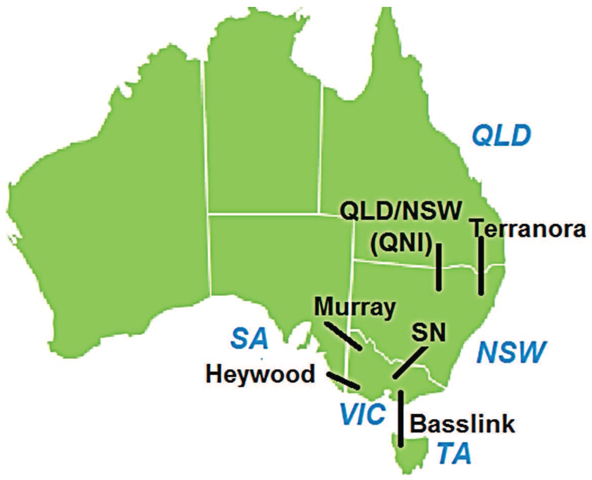
The four Australians markets selected in this study are New South Wales (NSW), Queensland (QLD), South Australia (SA) and Victoria (VIC). The Australian National Electricity Market (NEM) promotes efficient generation and demand use by a wholesale market, which allows electricity trade among five regions in the east of Australia (see Figure 1): Queensland (QLD); New South Wales (NSW); Snowy Mountains region (SN, abolished in 2008 and merged into VIC and NSW areas); Victoria (VIC); South Australia (SA); and Tasmania (TA, fully operational in NEM since 2006).

Each region has different characteristics (generation mix and load) and interconnection capacities. For example, New South Wales is a net importer of electricity and has limited capacity to cover the highest peaks of demand, and for this reason, it needs generation support from QLD, Snowy Hydro and VIC. Victoria had in the period under study (2004 to 2009) a substantial low cost base-load capacity, making it a net exporter of electricity. Queensland is a net exporter too, mainly to NSW, due to their geographical and electrical proximity. South Australia is a net importer (a high percent of its demand was covered outside this region until 2005–2006 because a new investment in wind generation was developed in this area).

Table 2. Inter-regional trade as a percentage of regional energy demand.

Region/Year	2004–2005		2005–2006		2006–2007		2007–2008
	Import	Export	Import	Export	Import	Export	Import	Export
QLD	-	9%	-	13%	-	14%	-	10%
NSW	11%	-	12%	-	11%	-	8%	-
VIC	-	6%	-	3%	-	4%	-	2%
SA	18%	-	20%	-	7%	-	-	-
TA	-	-	-	-	13%	-	22%	-

(adapted from [35]) shows the inter-regional trade of these regions.

The NEM market works at unison when the electricity can flow freely among all areas, but this does not mean that the price is the same in the five areas during these periods. The “integrity” or price alignment of the NEM market as a percentage of trading hours ranges between 70% and 80% across the regions. Australia manages congestion periods by splitting its regions, allowing different and more independent marginal prices in each area. This separation occurs when a transmission inter-connector becomes congested and limits inter-regional power flows. In these cases, each area needs to reconsider offers from the generation in its own region, and in this way, a different behavior of the market occurs in each area (the generation mix is different for each region). This scenario may occur at times of peak demand or when an inter-connector experiences some outage or is under maintenance tasks. The inter-connectors in Australia are shown in Figure 1. Notice that Australia does not have a meshed link among regions (QLD, NSW, SA, VIC, TA), but a radial one.

The Nord Pool markets are divided into several bidding areas. The available transmission capacity may vary and congest the flow of power between the bidding areas, and thereby, different area prices are established. For each Nordic country, the local transmission system operator (TSO) decides into which bidding areas the country is divided. The bidding areas has changed along time, and for the time period analyzed (the years 2004 to 2009), we have considered the following: Sweden (SE), Finland (FI), Western Denmark (DK1), Eastern Denmark (DK2), Oslo (NO1) and Trondheim (NO2). Nord Pool calculates a price for each bidding area for each hour of the following day. The Nord Pool System price (NPS) is calculated based on the sale and purchase orders disregarding the available transmission capacity between the bidding areas in the Nordic market.

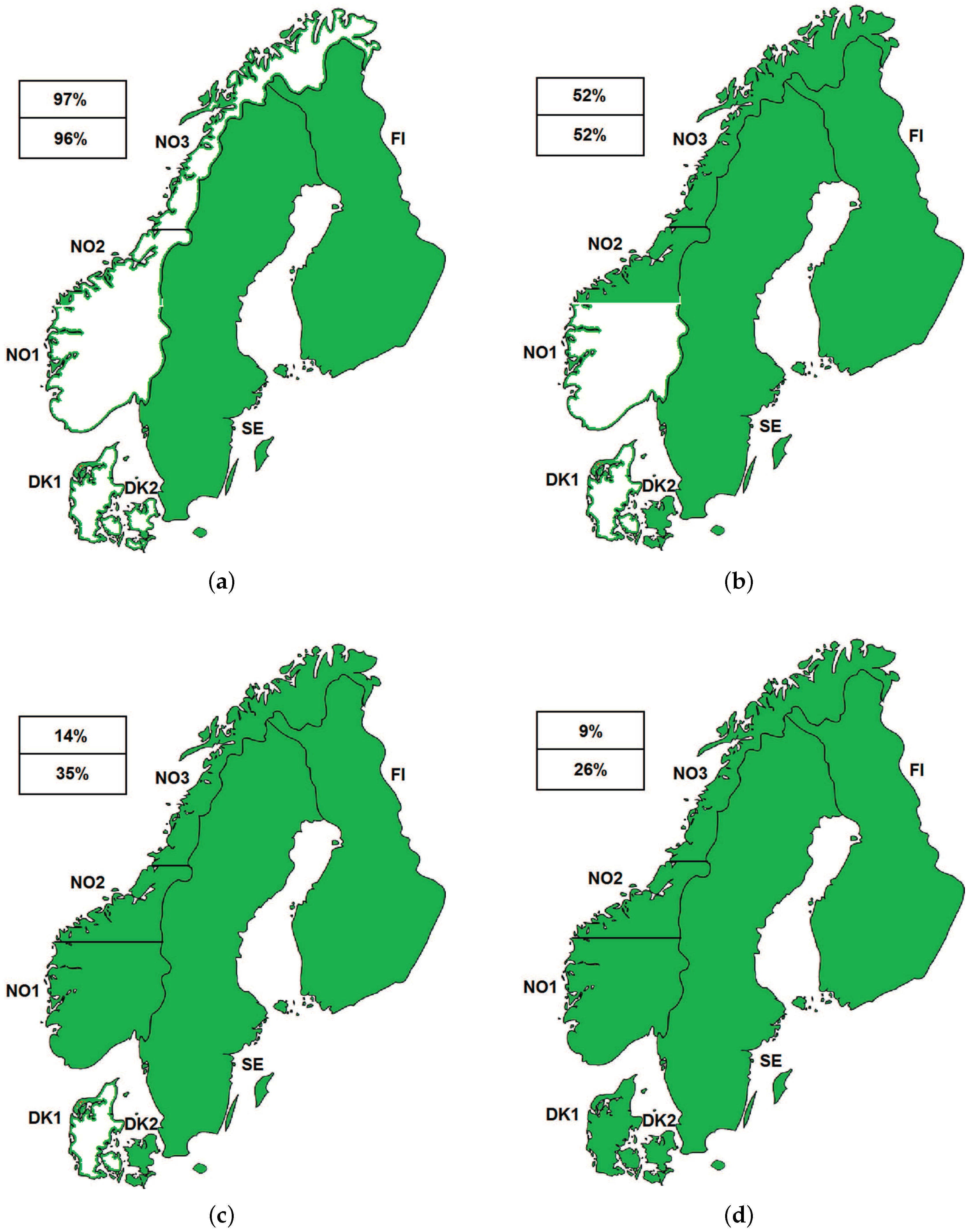
The Nordic area is a good example of a well-linked region. From the early 1990s, these countries made solid foundations for the development of a supra-national market, but despite this fact, the integrity of price areas is not the same (see Figure 2). The Nordic Transmission grid connects the four countries of this area, and the congestions between the countries are managed by implicit auctions through Nord Pool spot. The Nordic electricity grid has several AC and DC inter-connectors to link the different countries in the region and to interconnect adjacent areas. For example, in the period under study (2004 to 2009), the Denmark West- Germany corridor had 1500 MW and 950 MW in the opposite direction. Finland is strongly connected to Sweden (2050 MW Sweden-Finland and 1650 MW in the opposite direction), but weakly with North Norway (100 MW) and Estonia (in 2007 with a capacity of 350 MW). Finland forms its own bidding area. The weakest linked area is Western Denmark (DK1) because it was part of the Continental European synchronous power system, the former UCTE area (Union for the Coordination of the Transmission of Electricity) and now the Continental European Group of ENTSO-E (European Network of Transmission System Operators for Electricity), whereas Eastern Denmark (DK2) was part of the Nordic synchronous area (the former Nordel, now the Baltic Regional Group of ENTSO-E [36]). The second one, according to Figure 2, is the NO1 area (Oslo region) due the capacity problems of the west coast Swedish corridor. Moreover, the capacity usually available from SE to NO2 and NO3 is limited. The most coherent areas in the period analyzed were FI and SE due to the high transmission capacity between Finland and North Sweden.

3.2. Classification Results

For each electricity market, hourly price series from 2004 to 2009 are used in the analysis. The proposed measures allow us to determine which markets present strong relationships and which ones are not related. Furthermore, the strength of the relation can be measured along the year in order to detect periods with the most or the least price dependency.

For that, the whole time series has been divided into non-overlapping blocks of size w (block size), and then, given an embedding dimension m, the distance measures proposed in this paper are computed for each block. The block size selected when computing distance measures usually corresponds to a year approximately ($w=8760$ h) or to a season of the year ($w=2190$ h), because the proposed measures do not depend on the block size w, and we are interested in studying whether the dependency level is homogeneous along time. However, a suitable combination of embedding m and block size w should be chosen when developing the independency test. A general rule to get a good performance is that the block size w ought to be roughly $w=5$·5·$m!$·$m!$. For example, when the embedding dimension is $m=3$, a block size of $w=5$·5·$3!$·$3!$$=900$ is recommended. See [14] for more details.

Firstly, we highlight the necessity of removing the seasonal component before the analysis. Note that hourly electricity price series have daily and weekly seasonal components (period = 24 h and period = 168 h, respectively), and these seasonal parts are more relevant (higher values) than the stochastic part of the series. Taking into account this framework, we wondered if the dependence test was appropriate for series with a seasonal behavior. Let ${\left(x_t\right)}_{t=1}^{t=T}$ be the original price series of a specific electricity market. In this context, we consider three different ways to remove seasonality in the price series to extract the stochastic component:

• Taking weekly seasonal differences:

  $$y_t=x_t-x_{t-168}$$

  (24)
• First taking weekly seasonal differences and then daily differences:

  $$\begin{array}{ccc}\hfill y_t& =& x_t-x_{t-168}\hfill \end{array}$$

  (25)

  $$\begin{array}{ccc}\hfill z_t& =& y_t-y_{t-24}\hfill \end{array}$$

  (26)
• Using the method proposed in [37]:

  $$y_t=x_t-\left(\frac{1}{N}\sum _{i=1}^N{x}_{t-i·168}+\frac{1}{7}\sum _{j=1}^7{x}_{t-j·24}-\frac{1}{7N}\sum _{i=1}^N\sum _{j=1}^7{x}_{t-i·168-j·24}\right)$$

  (27)

  where $N+1=5$ is the number of weeks used for calibration. This approach is more popular among practitioners because it combines differencing at various lags with moving average smoothing.

Note that the the length of the resulting stochastic component is less than the length of the original series in all cases, because the first part of the data cannot be used.

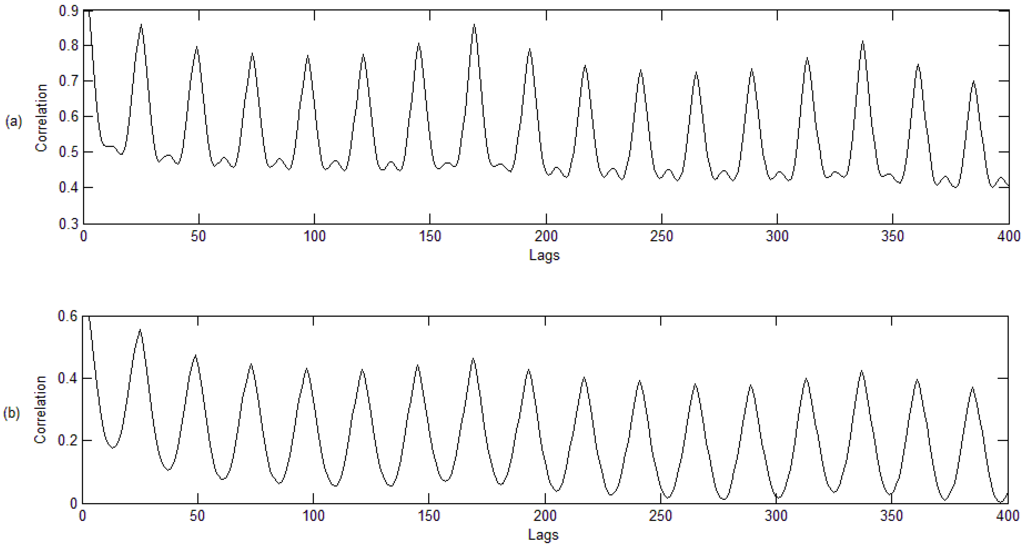
Let us consider the hourly price series in the whole period 2004 to 2009 of two very different electricity markets, Ontario and Omel, which are far away and have different market regulations. It is clear that the prices of both markets are independent, but the presence of seasonality leads to the wrong conclusion if the seasonal component is not previously removed. Figure 3 shows the correlograms of the two price series, which reveals clear daily and weekly seasonal components (peaks in Lags 24, 168 and their multiples).

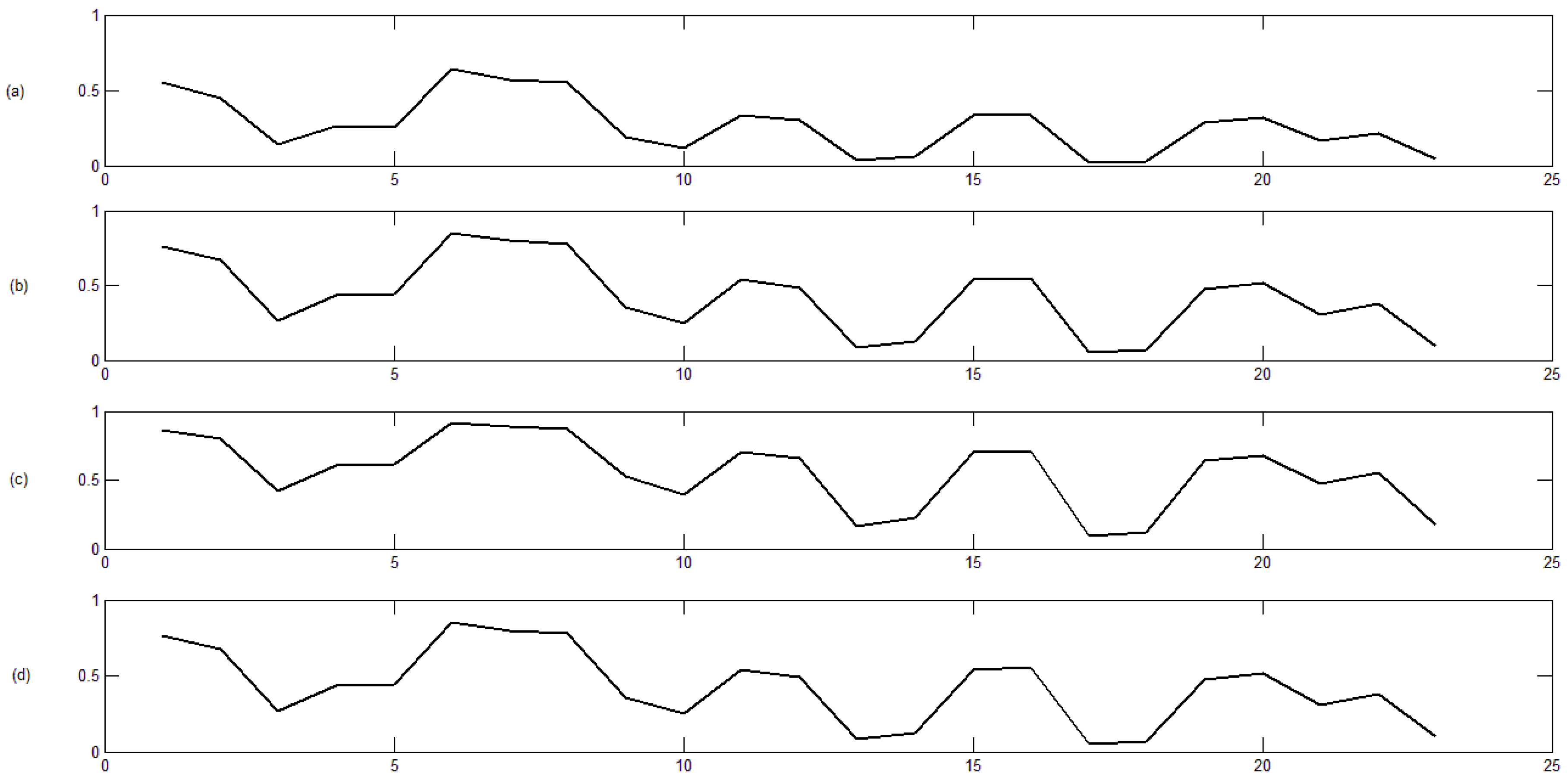
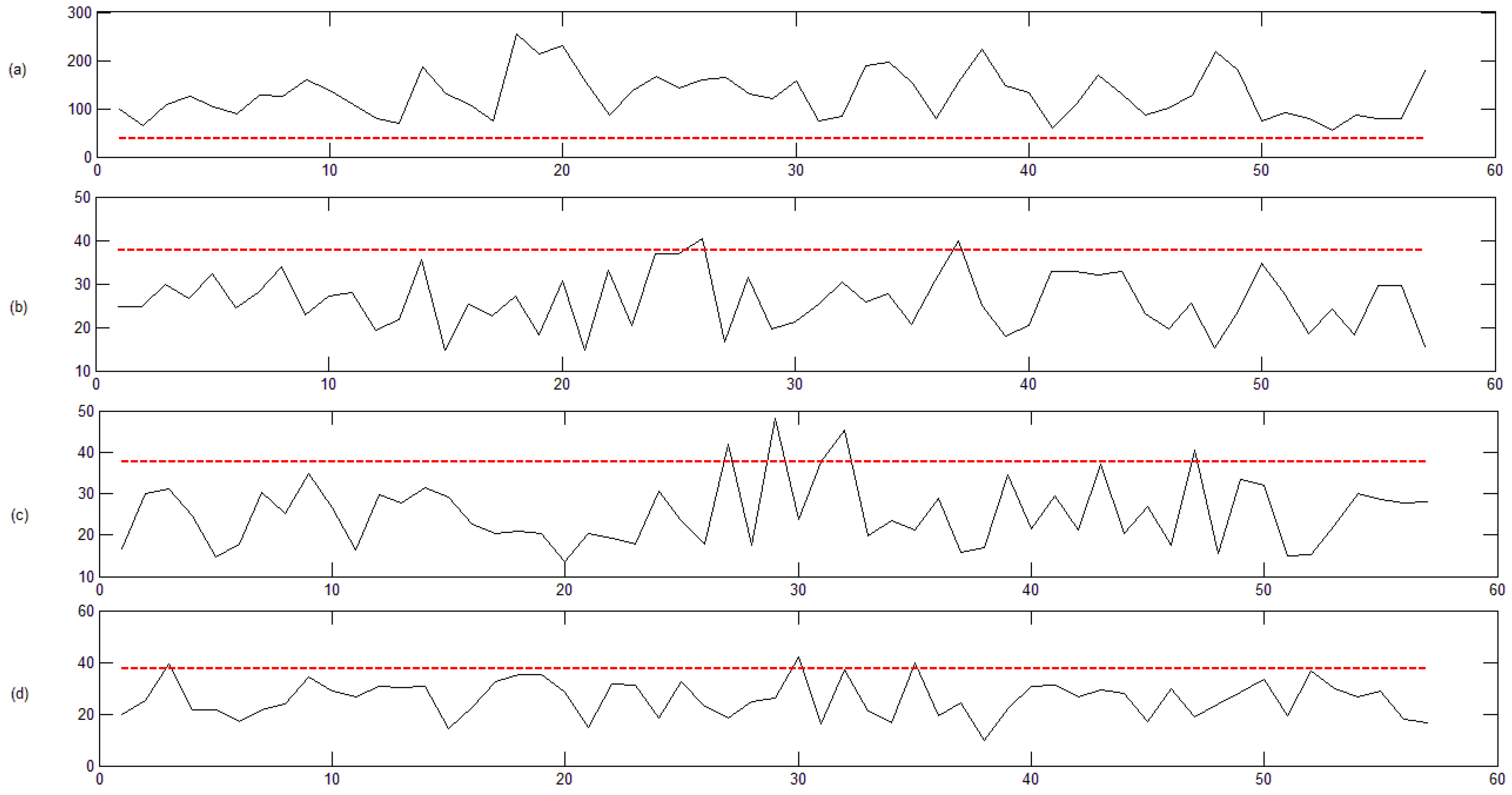
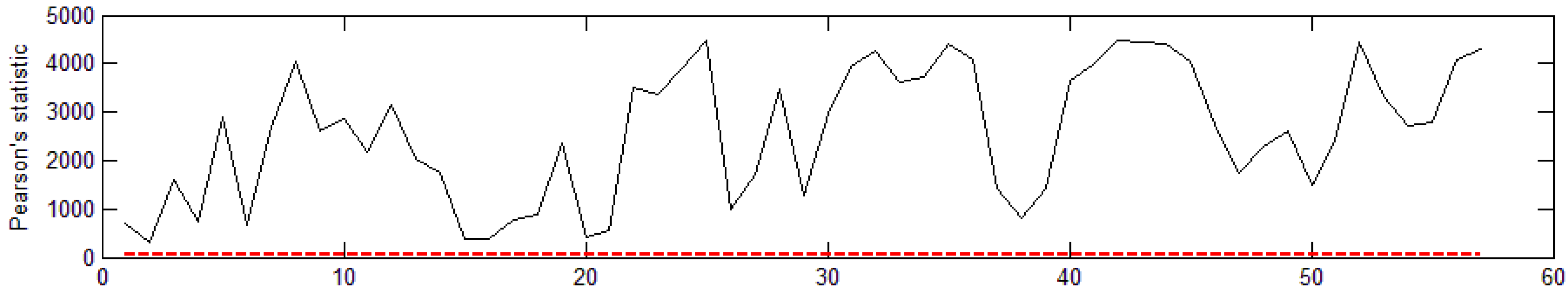
Now, we compute Pearson’s chi-squared, the likelihood-ratio and the Cressie–Read statistics in four different situations: using the original data (without removing the seasonal component) and using the stochastic component extracted in the three ways mentioned above. Figure 4 shows the results for Pearson’s chi-squared statistics (the others statistics were nearly the same), and the dotted line represents the limit of the rejection region. An embedding dimension of $m=3$ and a block size of $w=5·$$5·$$3!·$$3!=900$ were chosen for the test. When original data are considered (see Figure 4a), the statistic lays in the rejection region, so we would conclude that both price series are dependent. However, after removing the seasonal component with any method (see Figure 4b–d), the statistic states independency between the price series. The selection of $m=4$ and $w=5·$$5·$$4!·$$4!=$ 14,400 leads to the same conclusions.

In the rest of the paper, we have applied Weron’s method to all price series before each analysis, so the stochastic components of the price series have been used instead of the original data.

As we mentioned before, the proposed distance measurements can be used to study the strength of the dependency along time. To illustrate this task, let us consider the hourly price series of Finland and Sweden from 2004 to 2009, two electricity markets that are strongly related. First, we compute the dependency statistics with $m=3$ and $w=900$ to show a true price dependence between these two electricity markets; see Figure 5. Note that the resulting series are of a size of 51,768 h after applying Weron’s method, so there are 57 windows of a size of $w=900$ along the period analyzed.

An embedding dimension of $m=3$ and a block size of $w=2190$ (a season of the year, approximately) are now selected to evaluate how the dependency level varies along time. Note that the resulting series are of a size of 50,724 h after removing the seasonality through Weron’s procedure and starting in 21 March 2004 (spring). Therefore, there are 23 windows of a size of $w=2190$ along the period analyzed, from spring 2004 to autumn 2009. Figure 6 reveals that the dependency level is not homogenous along time. On the one hand, a slight increase of the dependency level can be appreciated along the years analyzed (distance presents a decreasing trend). On the other hand, there are some dependency peaks (valleys in the distance graph) in autumn of 2004, spring 2005, spring-summer of 2006, spring-summer of 2007, spring-summer of 2008 and autumn of 2009. Furthermore, note that the four distances provide a similar pattern, but the scales change, except for the uncertainty distance ($D_U$) and the Universal Distance 2 ($D_2$), which are roughly the same.

To explain, from a physical point of view, the results shown in Figure 6, it is interesting to consider two aspects. First, the fact that the share of electricity bought from the power exchange in relation to electricity consumption has increased considerably since Finland and Sweden joined the Nordic power market. For example in Finland, the share of electricity bought from the Nordic power exchange has increased from 5% to 60% of the Finnish consumption in 2012 [38]. 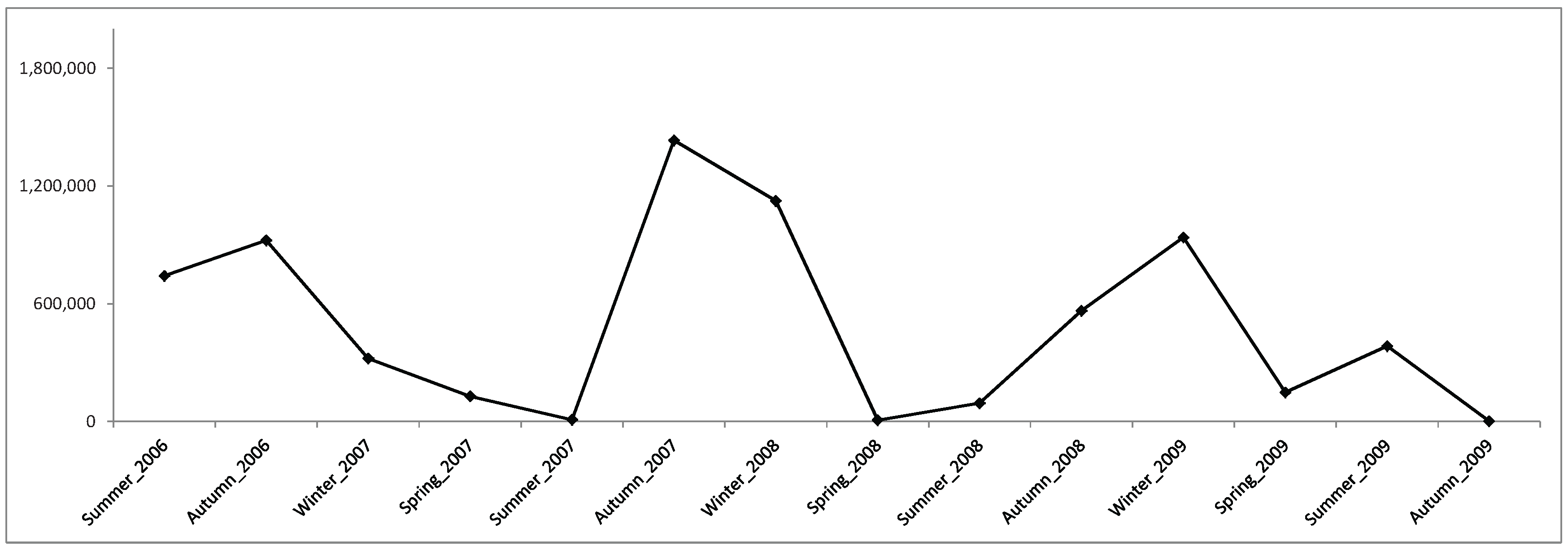This means a higher dependence (potentially) among Finland and Sweden (and, obviously, with the Nord Pool area) and explains the slight increase in dependency level along the period shown in Figure 6. The second is the management of congestions. In the Nordic area, two mechanisms are used: counter trade and congestion rents. The first is used with market agents to relieve both national and inter-regional congestions during the daily network operation. The cost of this mechanism in Finland decreased from 0.86 million euros in 2004 to 0.085 million euros in 2009 [39]. The second mechanism is the most important to evaluate cross-border congestions, the so-called congestion rents. Congestion rents come up in the situation where transmission capacity between bidding zones is not sufficient to fulfill the demand. The congestion splits the price bidding zones into separate price areas, and the power exchange and TSOs receive congestion income from the congested interconnection. The congestion rents are computed as the product of the commercial flow on the day ahead market and the difference of the area prices. In this way, high levels of congestion rents between two areas in some periods of time mean that these areas were more independent during those periods. Historical congestion rents between Finland and Sweden [39] have been analyzed (from summer of 2006 to autumn 2009), and they are shown in Figure 7. Note that the right part of Figure 6 (starting at window Number 10, which corresponds to summer 2006) and Figure 7 exhibit similar trend changes.

Finally, we study the dependence structure among all of the electricity markets analyzed. First, we compute the corresponding distance matrix, and then, we obtain the hierarchical classification of the markets. The distance matrices are computed for each one of the proposed distance measures ($D_V$, $D_U$, $D_1$ and $D_2$), for each year of the analyzed period (2004, 2005, 2006, 2007, 2008 and 2009) and for the whole period 2004 to 2009. An embedding dimension of $m=3$ is selected for individual years and $m=4$ for the six-year period. As examples,

Table 3. $D_V$ and $D_U$ distances for the period 2004 to 2009. NPS, Nord Pool System.

${\mathit{D}}_{\mathit{U}}$∖${\mathit{D}}_{\mathit{V}}$	NSW	QLD	SA	VIC	Aust	DK2	DK1	FIN	NPS	Omel	Onta	NO1	SE	NO2
NSW		0.65	0.77	0.65	0.98	0.98	0.98	0.98	0.97	0.97	0.98	0.98	0.98	0.98
QLD	0.75		0.86	0.8	0.98	0.98	0.98	0.98	0.98	0.98	0.98	0.98	0.98	0.98
SA	0.87	0.94		0.66	0.98	0.98	0.98	0.98	0.98	0.98	0.98	0.98	0.98	0.98
VIC	0.75	0.89	0.76		0.98	0.98	0.98	0.98	0.98	0.98	0.98	0.98	0.98	0.98
Aust	1	1	1	1		0.96	0.95	0.97	0.97	0.97	0.98	0.97	0.97	0.97
DK2	1	1	1	1	0.99		0.89	0.75	0.85	0.98	0.98	0.92	0.68	0.86
DK1	1	1	1	1	0.99	0.96		0.92	0.91	0.98	0.98	0.95	0.91	0.94
FIN	1	1	1	1	1	0.87	0.98		0.79	0.98	0.98	0.9	0.35	0.74
NPS	1	1	1	1	1	0.93	0.97	0.87		0.98	0.98	0.76	0.75	0.79
Omel	1	1	1	1	1	1	1	1	1		0.98	0.98	0.98	0.98
Onta	1	1	1	1	1	1	1	1	1	1		0.98	0.98	0.98
NO1	1	1	1	1	1	0.98	0.99	0.97	0.85	1	1		0.86	0.87
SE	1	1	1	1	1	0.82	0.97	0.48	0.82	1	1	0.94		0.63
NO2	1	1	1	1	1	0.94	0.99	0.85	0.87	1	1	0.95	0.76

and

Table 4. $D_1$ and $D_2$ distances for the period 2004 to 2009.

${\mathit{D}}_2$∖${\mathit{D}}_1$	NSW	QLD	SA	VIC	Aust	DK2	DK1	FIN	NPS	Omel	Onta	NO1	SE	NO2
NSW		0.86	0.93	0.86	1	1	1	1	1	1	1	1	1	1
QLD	0.75		0.97	0.94	1	1	1	1	1	1	1	1	1	1
SA	0.87	0.94		0.86	1	1	1	1	1	1	1	1	1	1
VIC	0.75	0.89	0.76		1	1	1	1	1	1	1	1	1	1
Aust	1	1	1	1		1	1	1	1	1	1	1	1	1
DK2	1	1	1	1	0.99		0.98	0.93	0.96	1	1	0.99	0.9	0.97
DK1	1	1	1	1	0.99	0.96		0.99	0.98	1	1	1	0.99	0.99
FIN	1	1	1	1	1	0.87	0.98		0.93	1	1	0.98	0.65	0.92
NPS	1	1	1	1	1	0.93	0.97	0.88		1	1	0.92	0.9	0.93
Omel	1	1	1	1	1	1	1	1	1		1	1	1	1
Onta	1	1	1	1	1	1	1	1	1	1		1	1	1
NO1	1	1	1	1	1	0.98	0.99	0.97	0.85	1	1		0.97	0.97
SE	1	1	1	1	1	0.82	0.97	0.48	0.82	1	1	0.94		0.86
NO2	1	1	1	1	1	0.94	0.99	0.85	0.88	1	1	0.95	0.76

show the distances between each pair of markets for the six-year period and

Table 5. $D_V$ and $D_U$ distances for year 2007.

${\mathit{D}}_{\mathit{U}}$∖${\mathit{D}}_{\mathit{V}}$	NSW	QLD	SA	VIC	Aust	DK2	DK1	FIN	NPS	Omel	Onta	NO1	SE	NO2
NSW		0.69	0.83	0.71	1	1	1	1	1	1	1	1	1	1
QLD	0.69		0.74	0.66	0.98	0.97	0.98	0.98	0.98	0.97	0.98	0.98	0.98	0.97
SA	0.83	0.92		0.44	0.98	0.98	0.97	0.98	0.98	0.98	0.98	0.97	0.97	0.98
VIC	0.71	0.86	0.65		0.98	0.97	0.98	0.98	0.98	0.98	0.98	0.97	0.97	0.98
Aust	1	1	1	1		0.94	0.93	0.96	0.95	0.97	0.97	0.97	0.96	0.97
DK2	1	1	1	1	0.99		0.77	0.72	0.8	0.97	0.98	0.91	0.69	0.79
DK1	1	1	1	1	0.99	0.93		0.9	0.85	0.97	0.98	0.96	0.88	0.93
FIN	1	1	1	1	1	0.91	0.99		0.68	0.97	0.98	0.83	0.19	0.52
NPS	1	1	1	1	1	0.95	0.97	0.87		0.97	0.97	0.7	0.65	0.69
Omel	1	1	1	1	1	1	1	1	1		0.97	0.97	0.98	0.98
Onta	1	1	1	1	1	1	1	1	1	1		0.98	0.98	0.98
NO1	1	1	1	1	1	0.99	1	0.96	0.89	1	1		0.81	0.8
SE	1	1	1	1	1	0.89	0.98	0.36	0.84	1	1	0.96		0.44
NO2	1	1	1	1	1	0.95	0.99	0.75	0.87	1	1	0.95	0.67

and

Table 6. $D_1$ and $D_2$ distances for year 2007.

${\mathit{D}}_2$∖${\mathit{D}}_1$	NSW	QLD	SA	VIC	Aust	DK2	DK1	FIN	NPS	Omel	Onta	NO1	SE	NO2
NSW		0.82	0.91	0.83	1	1	1	1	1	1	1	1	1	1
QLD	0.7		0.96	0.92	1	1	1	1	1	1	1	1	1	1
SA	0.83	0.92		0.79	1	1	1	1	1	1	1	1	1	1
VIC	0.71	0.86	0.65		1	1	1	1	1	1	1	1	1	1
Aust	1	1	1	1		1	1	1	1	1	1	1	1	1
DK2	1	1	1	1	0.99		0.96	0.95	0.97	1	1	0.99	0.94	0.97
DK1	1	1	1	1	0.99	0.93		0.99	0.98	1	1	1	0.99	1
FIN	1	1	1	1	1	0.91	0.99		0.93	1	1	0.98	0.53	0.86
NPS	1	1	1	1	1	0.95	0.97	0.87		1	1	0.94	0.91	0.93
Omel	1	1	1	1	1	1	1	1	1		1	1	1	1
Onta	1	1	1	1	1	1	1	1	1	1		1	1	1
NO1	1	1	1	1	1	0.99	1	0.96	0.89	1	1		0.98	0.97
SE	1	1	1	1	1	0.89	0.98	0.36	0.84	1	1	0.96		0.8
NO2	1	1	1	1	1	0.95	0.99	0.75	0.87	1	1	0.95	0.67

for the individual year 2007.

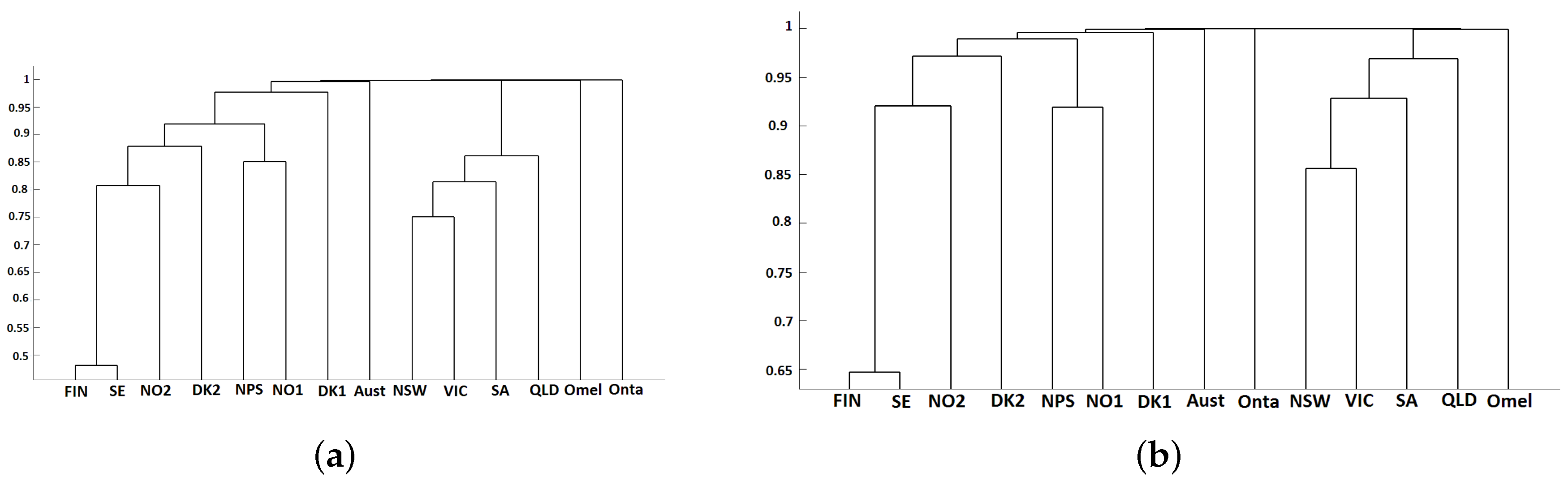
The hierarchical clustering of the electricity markets has been developed from the previous distance matrices and using different linkages (single, complete and average). For instance, Figure 8 shows the classification results for the whole six-year period, V-Cramer distance and single linkage. Dendrograms for all distance measurements and all linkages reveal the same hierarchical classification. Four clusters can be distinguished: two of them are isolated markets (Omel and Ontario, respectively); the third one consists of the four Australian regions (Victoria, New South Wales, South Australia and Queensland); and the forth cluster includes all Nord Pool regions (Finland, Sweden, Trondheim, Oslo, East Denmark, West Denmark and the system) together with Austria. Note that West Denmark is weakly related to the rest of the Nordic countries, whereas Finland and Sweden have the strongest price dependency.

Note that the clustering approach proposed in this paper produces plausible, non-trivial results that can be intuitively explained in the given scenario. Obviously, the final classification results depend on several aspects jointly, such as the size of the regions, the system’s regulation laws, demand daily patterns, costs for the spinning reserve or fees for cross-border energy transmission. Below, we try to highlight some aspects that partially justify the clustering results in spite of the fact that it is not the aim of the work.

The isolation of the Ontario market in this analysis does not need any comment, and the one of the Spanish market is also well known. For instance, the capacity of cross-border connection from Spain to France in 2008 was only 1400 MW (3% of Spanish demand), and France did not join the European Power Exchange (EPEX) initiative until 2009 to 2010, as well. According to the European Association of Regulators (ACER), up to 2010, the percentage of hours for equal hourly day-ahead prices in the pair France-Germany was 0%. In this way, Spain had no possibility of economic or physical linkage with other European markets, such us Nord Pool or Austria, outside the limited possibility of exchange with France. Therefore, it is very unlikely that Omel and Nord Pool had been linked through EPEX (via France-Germany) during that period. On the other side, the dendrograms reveal that Austria exhibits a weak dependence with Denmark areas. This is due to the fact that Austria and Denmark areas (DK1 and DK2) are linked through Germany. Austria has a high capacity of cross-border lines with Germany (10020 MW and 3664 MW in 2009). However, from 2004 to 2008, the energy volume traded by the Energy Spot Market in Austria (EXAA), which covers German areas) did not get 7% with respect to Austrian overall demand [40]. In September 2008, the EPEX (Germany-Austria) was founded, but in its first year, it traded less than 17% of the Austrian gross demand of electricity. Hence, the market integration was very weak in that period.

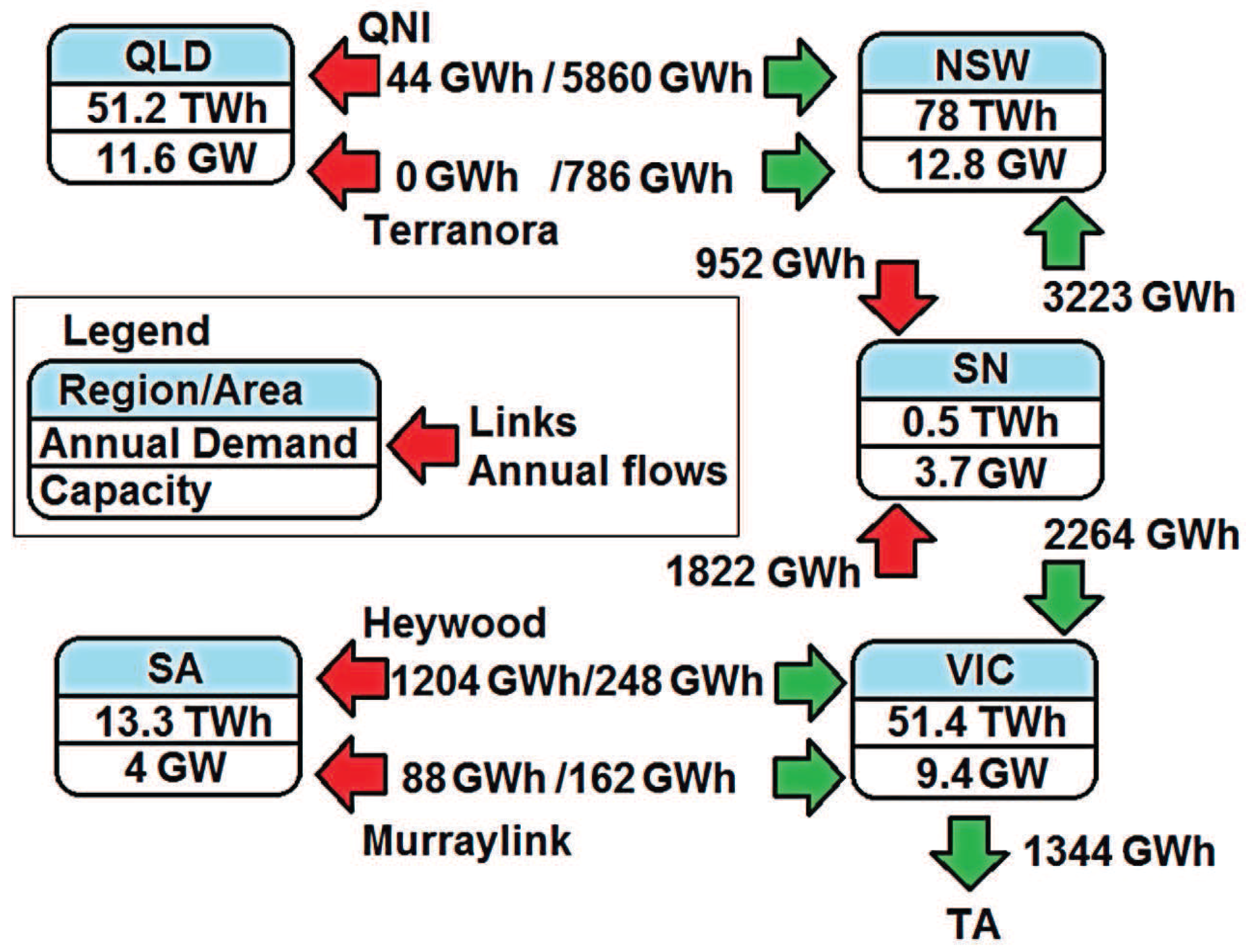
The results obtained for the Nordic regions are in agreement with the integrity levels showed in Figure 2, where DK1 has the lowest integrity percentage with the rest of regions, whereas FI and SE have the highest one. To explain the hierarchical classification in the case of Australia, two aspect can be considered: first, inter-connectors’ capacity and their constraints, and second, the annual power flows between Australian areas. With respect to annual power flows between areas, Figure 9 shows a snapshot of the NEM market for 2006/2007 (adapted from [41]). This figure and the above-mentioned conditions of transmission inter-connectors and physical energy exchanges among regions can explain the distance matrices and dendrograms. From these power flows, it can be seen that NSW needs support from QLD and VIC. On the other side, QLD has a sufficient amount of generation in its area (the area is more independent), and its dependency with VIC and SA is lower than the link with NSW. Finally, SA needs imports from VIC (a net exporter area), but not from NSW (a net importer from VIC and QLD).

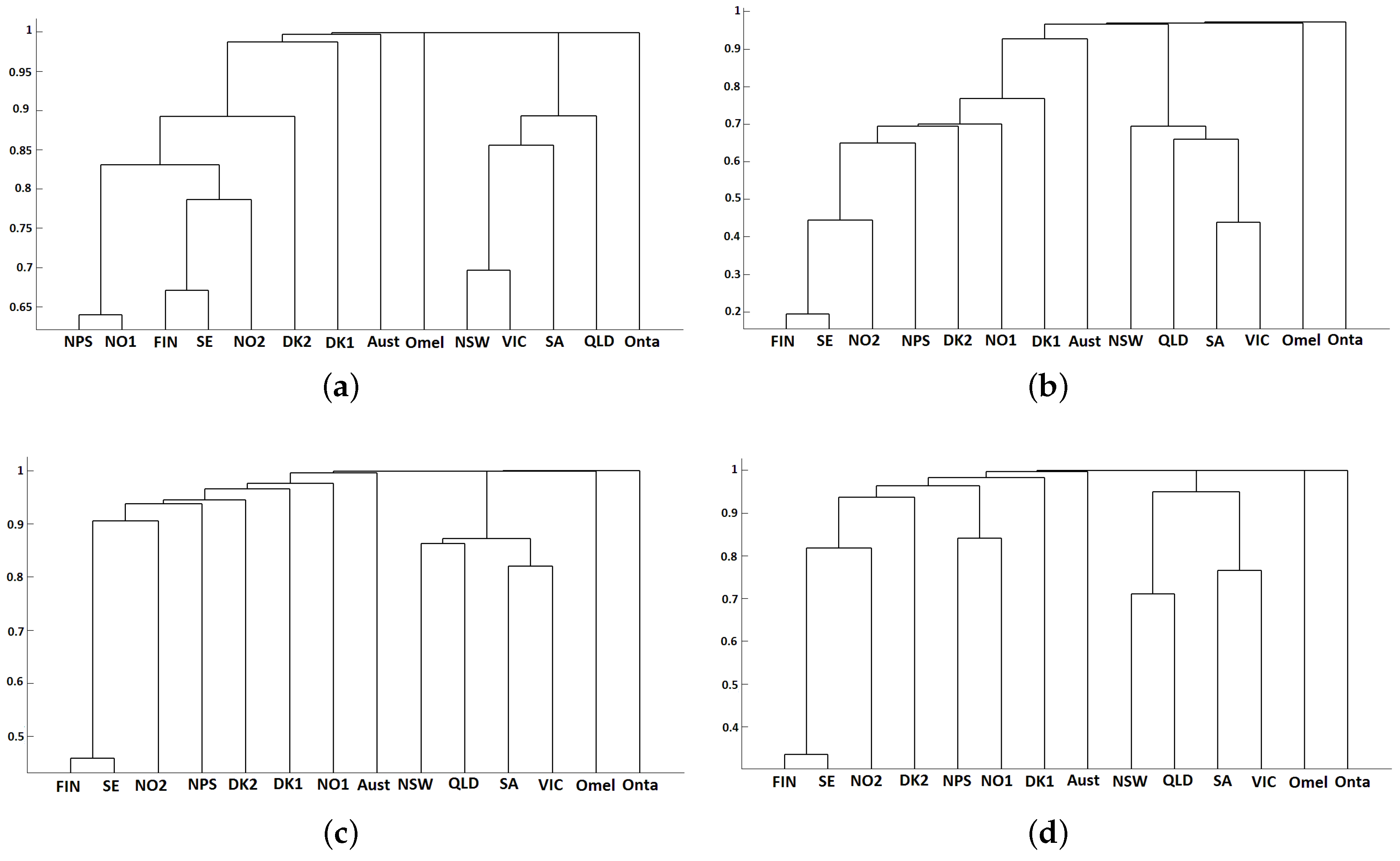
In general, dendrograms for each individual year lead to clustering results similar to that of the six-year period, but some differences are worth being outlined (see Figure 10). For instance, in 2005, there was a strong dependence between prices of Nord Pool’s system and Oslo (even higher than the dependence level between Finland and Sweden). In 2008, the dependency strength of Oslo’s region with the rest of the Nordic regions went down, and it became the weakest (even lower than the association of West Denmark with the rest of the regions). In that year, the hydropower production in Norway was higher to compensate lower Swedish production (because the availability of nuclear power plants in Sweden went down during 2008, reaching 65% during some months, especially in November and December) and also due to some problems with the imports from the Central-West European area [42]. Both facts originated congestion problems with the transmission inter-connectors and a loss of price integrity in the NO1 area. Finally, the dependence scheme of the four Australian regions has been changing along the years: in 2005 and 2006, NSW and VIC were the most related; in 2007 and 2008, the highest dependency went to the couple SA and VIC; but in 2009, NSW and QLD reached the maximum dependence level.

Although we have focused on electricity prices, the proposed approach could be helpful to study the relationships among other kinds of time series like electricity loads. Below, we consider a set of twelve time series corresponding to the hourly electricity loads in four different regions along three different years (2007, 2008 and 2009). Specifically, we have analyzed the electricity load series of three regions in Australia: New South Wales (NSW), South Australia (SA) and Victoria (VIC); and the load time series of Ontario’s market. The objective is to apply the proposed clustering procedure to this set of time series in order to obtain groups of series that present dependency among themselves.

Recall that the steps of the procedure can be summarized as follows:

• First, the seasonal component of the time series must be removed. We suggest using Weron’s method given in (27), but other techniques can be applied.
• Secondly, the resulting time series (after removing the seasonal component) are codified by means of permutations. For that, the researcher has to choose the embedding dimension.
• Thirdly, the distance between each pair of time series (through their codes) is computed, and the corresponding distance matrix is obtained. In this step, we propose using four different dissimilarity measures ($D_V$, $D_U$, $D_1$ and $D_2$).
• Finally, the dendrogram is computed obtaining the clustering results. For that, the researcher has to choose the distance measure and the linkage of the hierarchical method.

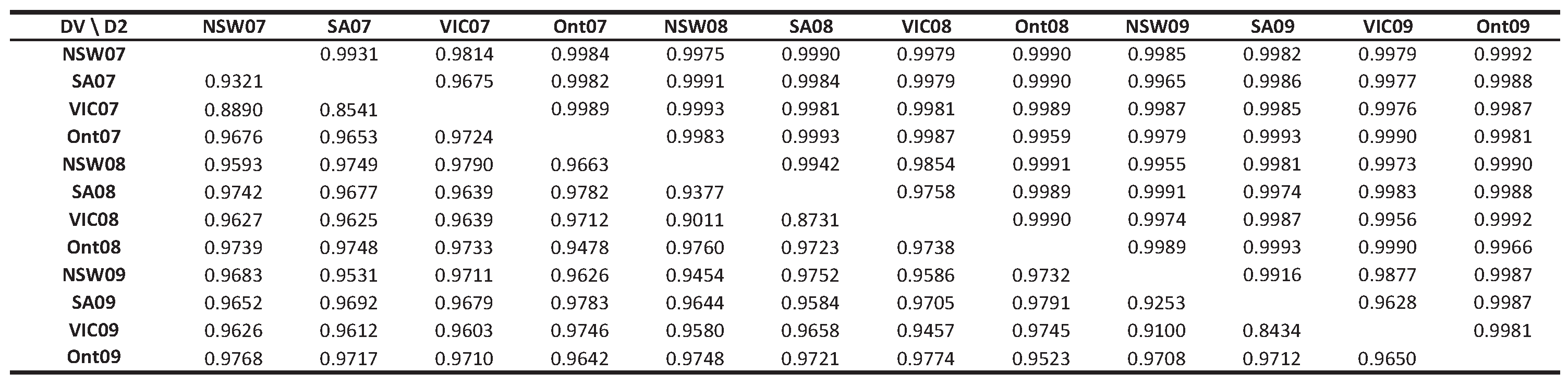
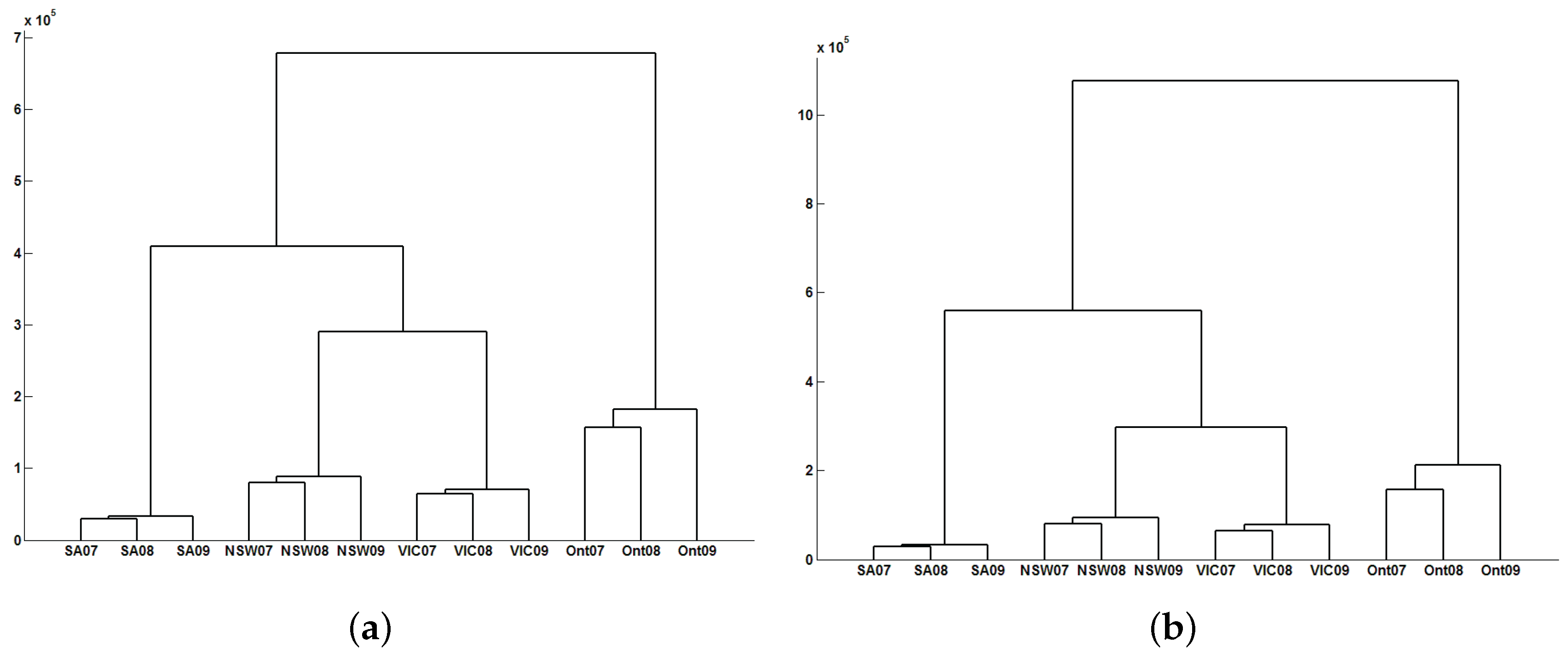
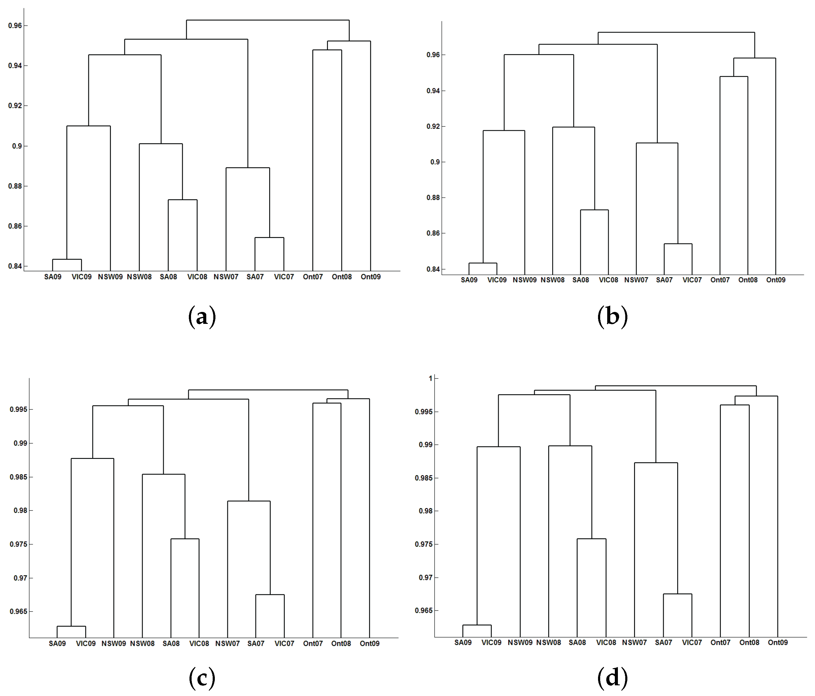
Once we have removed the seasonal component of each time series and we have codified the resulting series, we compute the distance matrices. Figure 11 shows the distance matrices (Crammer’s V distance and Universal Distance 2) of the twelve time series, using embedding dimension $m=3$. Additionally, Figure 12 shows the corresponding classification results choosing different linkages. The electricity loads of New South Wales for 2007, 2008 and 2009 are denoted by NSW07, NSW08 and NSW09, respectively, and similar notation is used for South Australia (SA07, SA08 and SA09), Victoria (VIC07, VIC08 and VIC09) and Ontario (Ont07, Ont08 and Ont09).

In Figure 12, two different clusters can be seen: the first one formed by the three load series of Ontario’s market and the second one formed by the nine load series of the Australian market. Moreover, in the second cluster, there are three subgroups that are well separated, one for each year analyzed. Therefore, we can state that the strength of dependency is greater among the Australian regions (NSW, SA and VIC) for a specific year than among the years for a specific region.

In each of the three subgroups of the Australian cluster, we can see that the strongest dependency corresponds to the load series of South Australia and Victoria, whereas New South Wales has the weakest dependency inside its subgroup. On the other hand, the three load series of Ontario present a weak dependency level among them, but high enough to create a different cluster from the Australian load series.

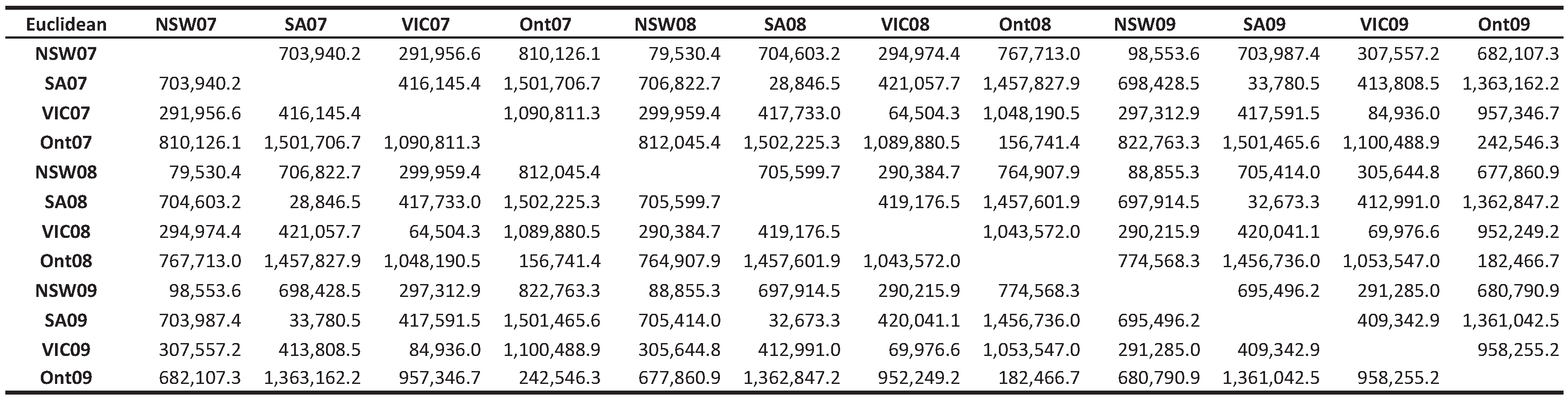
Finally, we compare some of our results with those obtained using a classical clustering approach for time series: a raw data-based approach and the Euclidean distance. In this case, we work directly with the original data, that is the time series are neither transformed nor codified. Additionally, the Euclidean distance is used as a dissimilarity measure, which is combined with different linkages. Figure 13 shows the Euclidean distance matrix of the twelve time series also considered in Figure 11. Recall that the Euclidean distance is not upper bounded; it is very sensitive to transformations; and the proximity notion relies on the closeness of the values observed at corresponding points of time.

Figure 14 shows the corresponding clustering results for the electricity loads of Ontario and Australia over different years.

Once again, two clusters can be distinguished: one composed of Ontario’s loads and the other one composed of the Australian loads. However, when we compare Figure 12 with Figure 14, an essential difference can be observed. This time, the cluster of the Australian loads is divided into three subgroups corresponding to each region analyzed. Therefore, if we classify this set of time series according to the information that they share (using the clustering approach proposed in the present paper), we get that the strength of dependency is greater among the regions (for each specific year), whereas if we classify them looking for similarities in time, we get that the similarity in time is greater among the years (for each specific region). This example illustrates the importance of choosing a suitable clustering approach and dissimilarity measure depending on the classification purpose.

4. Conclusions

The problem of time series clustering has great interest and applications in many disciplines. For instance, in the field of electricity markets, the study of relations among price time series becomes essential to give a first indicator of the degree of market integration.

The present paper proposes a novel approach in time series clustering, where the aim is to classify the series into homogeneous groups according to the dependency level among them. That is, given a set of time series, the proposed clustering method creates groups of time series that are related. The new approach combines three aspects: a permutation-based coding of the time series, distance measures that quantify dependencies between two discrete distributions and different linkages for hierarchical clustering. It is able to detect linear and nonlinear relationships, due to the nature of the symbolic representation of the time series done in the codifying stage.

The method was applied to several electricity markets from Europe, North America and Australia to illustrate its performance, using electricity prices and electricity loads, as well. We show that the proposed method produces plausible, non-trivial results that can be intuitively explained in the given scenario. Furthermore, some of our results were compared with those obtained using a raw data-based approach and the Euclidean distance, exhibiting the importance of choosing an appropriate approach depending on the clustering target.

Therefore, the method developed in this paper allows the researcher to classify a set of time series according to the degree of information that they share, creating groups of time series that are linear or non-linear dependent. On the other hand, some practical examples show the necessity of removing the seasonal component of the series before the analysis and the utility of this approach to study the variation of the dependency level between two price series along time.

References

1. European Added Value Unit (European Parliamentary Research Service, PE 536.364). Mapping the Cost of Non-Europe, 2014–2019 (April 2015). Available online: http://www.europarl.europa.eu (accessed on 22 May 2016).
2. European Added Value Unit (European Parliamentary Research Service, PE 504.466). Cost of Non-Europe in the Single Market for Energy. Annex IV. Benefits of an Integrated European Electricity Market: The Role of Competition (June 2013). Available online: http://www.europarl.europa.eu (accessed on 22 May 2016).
3. Australian Energy Regulator. National Electricity Market. Chapter 1. 2009. Available online: https://www.aer.gov.au/system/files/Chapter1Nationalelectricitymarket2009.pdf (accessed on 22 May 2016). [Google Scholar]
4. Australian Energy Regulator. National Electricity Market. Chapter 2. 2009. Available online: https://www.aer.gov.au/system/files/Chapter2Nationalelectricitymarket2009.pdf (accessed on 22 May 2016).
5. Erni, D. Cointegration in Spot Price Energy Markets. Master’s Thesis, University of St. Gallen (HSG), St. Gallen, Switzerland, 2009. [Google Scholar]
6. Mihaylova, I. Stochastic Dependencies of Spot Prices in the European Electricity. Master’s Thesis, University of St. Gallen (HSG), St. Gallen, Switzerland, 2009. [Google Scholar]
7. Bosco, B.; Parisio, L.; Pelagatti, M.; Baldi, F. Long-run relations in european electricity prices. J. Appl. Econom. 2010, 25, 805–832. [Google Scholar] [CrossRef]
8. Bollino, C.A.; Ciferri, D.; Polinori, P. Integration and convergence in European electricity markets. Munich Pers. RePEc Arch. 2013, 1–16. [Google Scholar] [CrossRef] [Green Version]
9. Haugh, L.D. Checking the independence of two covariance stationary time series: A univariate residual cross-correlation approach. J. Am. Stat. Assoc. 1976, 71, 378–385. [Google Scholar] [CrossRef]
10. Hong, Y. Testing the independence between two covariance stationary time series. Biometrika 1986, 83, 615–625. [Google Scholar] [CrossRef]
11. Cánovas, J.S.; Guillamón, A.; Ruiz, M.C. Using permutations to detect dependence between time series. Phys. D Nonlinear Phenom. 2011, 240, 1199–1204. [Google Scholar] [CrossRef]
12. Bandt, C.; Pompe, B. Permutation entropy: A natural complexity measure for time series. Phys. Rev. Lett. 2002, 88. [Google Scholar] [CrossRef] [PubMed]
13. Bruzzo, A.A.; Gesierich, B.; Santi, M.; Tassinari, C.A.; Birbaumer, N.; Rubboli, G. Permutation entropy to detect vigilance changes and preictal states from scalp EEG in epileptic patients. A preliminary study. Neurol. Sci. 2008, 29, 39–45. [Google Scholar] [CrossRef] [PubMed]
14. Cánovas, J.S.; Guillamón, A.; Ruiz, M.C. Using permutations to find structural changes in time series. Fluct. Noise Lett. 2011, 10, 13–30. [Google Scholar] [CrossRef]
15. Ruiz, M.C.; Guillamón, A.; Gabaldón, A. A new approach to measure volatility in energy markets. Entropy 2012, 14, 74–91. [Google Scholar] [CrossRef]
16. Liao, T.W. Clustering of time series data—A survey. Pattern Recognit. 2005, 38, 1857–1874. [Google Scholar] [CrossRef]
17. Aghabozorgi, S.; Shirkhorshidi, A.S.; Wah, T.Y. Time-series clustering—A decade review. Inf. Syst. 2015, 53, 16–38. [Google Scholar] [CrossRef]
18. Böckers, V.; Heimeshoff, U. The extent of the European power markets. Energy Econ. 2014, 46, 102–111. [Google Scholar] [CrossRef]
19. Izakian, H.; Pedrycz, W.; Jamal, I. Fuzzy clustering of time series data using dynamic time warping distance. Eng. Appl. Artif. Intell. 2015, 39, 235–244. [Google Scholar] [CrossRef]
20. Iglesias, F.; Kastner, W. Analysis of Similarity Measures in Times Series Clustering for the Discovery of Building Energy Patterns. Energies 2013, 6, 579–597. [Google Scholar] [CrossRef]
21. Möller-Levet, C.S.; Klawonn, F.; Cho, K.H.; Wolkenhauer, O. Fuzzy clustering of short time-series and unevenly distributed sampling points. Adv. Intell. Data Anal. 2003, 330–340. [Google Scholar]
22. Foster, E.D. State Space Time Series Clustering Using Discrepancies Based on the Kullback-Leibler Information and the Mahalanobis Distance. Ph.D. Thesis, University of Iowa, Iowa City, IA, USA, 2012. [Google Scholar]
23. Lin, J.; Keogh, E.; Wei, L.; Lonardi, S. Experiencing SAX: A novel symbolic representation of time series. Data Min. Knowl. Discov. 2007, 15, 107–144. [Google Scholar] [CrossRef]
24. Wallis, S. Measures of Association for Contingency Tables; University College London: London, UK, 2012. [Google Scholar]
25. Strehl, A.; Ghosh, J. Cluster Ensembles—A Knowledge Reuse Framework for Combining Multiple Partitions. J. Mach. Learn. Res. 2002, 583–617. [Google Scholar]
26. Yao, Y. Information-theoretic measures for knowledge discovery and data mining. In Entropy Measures, Maximum Entropy and Emerging Applications; Springer: Berlin, Germany, 2003; pp. 115–136. [Google Scholar]
27. Witten, I.H.; Frank, E. Data Mining: Practical Machine Learning Tools and Techniques; Morgan Kaufmann: Amsterdam, The Netherland, 2005. [Google Scholar]
28. Kraskov, A.; Stögbauer, H.; Andrzejak, R.G.; Grassberger, P. Hierarchical Clustering Based on Mutual Information. Biol. Phys. 2003, 1–11. [Google Scholar]
29. Nord Pool Spot. Available online: http://www.nordpoolspot.com (accessed on 3 March 2015).
30. Independent Electricity System Operator of Ontario Market Web Page. Available online: http://www.theimo.com/imoweb/marketdata/marketData.asp (accessed on 3 March 2015).
31. Australian Energy Market Operator Web Page. Available online: http://www.aemo.com.au/data/price_demand.html (accessed on 3 March 2015).
32. The Iberian electricity spot Market Operator (OMIE). Available online: http://www.omie.es (accessed on 3 March 2015).
33. Energy Exchange Austria (EXAA). Webpage of the Energy Exchange Austria. Available online: http://www.exaa.at (accessed on 3 March 2015).
34. European Commission. Commission Decision of 14.4.2010 relating to a proceeding under Article 102 of the Treaty on the Functioning of the European Union and Article 54 of the EEA Agreement (Case 39521-Swedish Interconnectors). 2010. Available online: http://ec.europa.eu/competition/antitrust/cases/dec-docs/39351/39351-1211-8.pdf (accessed on 25 July 2016).
35. Australian Energy Market Commission (AEMC). Congestion Management Review (Final Report, June 2008). Available online: http://www.aemc.gov.au/getattachment/ed17404e-3a72-491f-a579-b92aaddace36/Final-Report.aspx (accessed on 22 May 2016).
36. ENTSO-E (European Network of Transmission System Operators for Electricity). Available online: https://www.entsoe.eu/Pages/default.aspx (accessed on 22 May 2016).
37. Weron, R. Modeling and Forecasting Electricity Loads and Prices: A Statistical Approach; Wiley: Chichester, UK, 2006. [Google Scholar]
38. Energy Authority. National Report 2014. Available online: https://www.energiavirasto.fi/documents/10179/0/ National+Report+2014+Finland+1602-601-2014+-+20140710.pdf/61dd1249-c1d7-4b15-8af6-e2ce41f8dcd9?version=1.0 (accessed on 22 May 2016).
39. Fingrid (Transmission System Operator in Finland). Available online: http://www.fingrid.fi/en/Pages/default.aspx (accessed on 22 May 2016).
40. Energie Control Austria, E-Control (Austrian regulator). Market Report 2010: National Report to the European Commission. Available online: http://www.e-control.at (accessed on 22 May 2016).
41. NERA Economic Consulting. The Wholesale Electricity Market in Australia. A Report to the Australian Energy Market Commission (March 2008). Available online: http://www.aemc.gov.au/ (accessed on 22 May 2016).
42. Nordic Energy Regulators. NorREG Report on the Price Peaks in the Nordic Wholesale Market During Winter 2009–2010 (Report 1/2011). Available online: http://www.nordicenergyregulators.org/publications (accessed on 22 May 2016).
Figure 1. Australia National Electricity Market (NEM), regions and inter-connectors (lines in the figure). QLD, Queensland; SA, South Australia; VIC, Victoria; NSW, New South Wales; TA, Tasmania; SN, Snowy inter-connector; QNI, Queensland to New South Wales inter-connector.
Energies 09 00809 g001
Figure 2. Integrity of price areas in Nord Pool in 2008 and 2009. In the top of each rectangle, the percentage of "integrating" time for the year 2008, in the bottom, the percentage for the year 2009. DK, Denmark; SE, Sweden; FI, Finland; NO, Norway. (a) Percentage of integrity for SE and FI (green areas); (b) Percentage of integrity for SE, FI, DK2, NO2 and NO3; (c) Percentage of integrity for SE, FI, DK2, NO2, NO3 and NO1; (d) Percentage of integrity for SE, FI, DK2, NO2, NO3, NO1 and DK1.
Energies 09 00809 g002
Figure 3. Correlograms for the period 2004 to 2009: (a) Omel market; (b) Ontario market.
Energies 09 00809 g003
Figure 4. Independency tests between Omel and Ontario markets using Pearson’s chi-squared statistic (y-axes) in four different situations: (a) using original price data; (b) removing the seasonal component using Equation (24); (c) removing the seasonal component using Equation (26); (d) removing the seasonal component using Equation (27).
Energies 09 00809 g004
Figure 5. Independency test between the Finland and Sweden markets after removing the seasonal component through Equation (27).
Energies 09 00809 g005
Figure 6. Distance measures between Finland and Sweden markets for each season in 2004 to 2009. (a) D V distance; (b) D U distance; (c) D 1 distance; (d) D 2 distance.
Energies 09 00809 g006
Figure 7. Congestion rents from Finland to Sweden, in euros.
Energies 09 00809 g007
Figure 8. Dendrograms for the whole period 2004 to 2009. (a) D 1 distance and average linkage; (b) D 2 distance and complete linkage.
Energies 09 00809 g008
Figure 9. Snapshot of the NEM market (Australia).
Energies 09 00809 g009
Figure 10. Dendrograms for individual years. (a) D 2 and average linkage, 2005; (b) D V and single linkage, 2007; (c) D 1 and single linkage, 2008; (d) D U and complete linkage, 2009.
Energies 09 00809 g010
Figure 11. Distances D V and D 2 for electricity load series. Ont, Ontario; 07, 2007; 08, 2009; 09, 2009.
Energies 09 00809 g011
Figure 12. Dendrograms for electricity load series. (a) D V and single linkage; (b) D V and average linkage; (c) D 2 and single linkage; (d) D 2 and average linkage.
Energies 09 00809 g012
Figure 13. Euclidean distance for electricity load series.
Energies 09 00809 g013
Figure 14. Dendrograms for electricity load series: a raw data-based approach. (a) Euclidean distance and single linkage; (b) Euclidean distance and average linkage.
Energies 09 00809 g014