Switching Control of Wind Turbine Sub-Controllers Based on an Active Disturbance Rejection Technique

Abstract

Wind power generation systems require complex control systems with multiple working conditions and multiple controllers. Under different operating conditions, switching without disturbance between the sub-controllers plays a critical role in ensuring the stability of power systems. The sub-controllers of two typical cases in the permanent magnet direct drive (PMDD) wind turbine running process are studied, one is the proportional integral (PI) controller in the maximum power points tracking (MPPT) stage, the other is the fuzzy pitch angle controller in the constant power stage. The switching strategy of the two sub-controllers is the emphasis in this research. Based on the active disturbance rejection control (ADRC), the switching mode of the sub-controllers is proposed, which can effectively restrain the sudden changes of the rotor current during the switching process, and improve the quality of power generation. The feasibility and effectiveness of the sub-controller switching strategy is verified by Matlab/Simulink simulation for a 2 MW PMDD wind turbine.

1. Introduction

Wind energy is a kind of clean and renewable energy. With the increased public concern nowadays about the issues of energy and the environment, its development has been very rapid. Data from the Global Wind Energy Council shows that in 2015, the world’s new installed wind power capacity was 63,013 MW, and the annual growth rate was up to 22%. Global cumulative installed capacity reached 432,419 MW at a compound growth rate of 17% per year [1]. The European Union, the United States and China are the fastest developing regions and countries in the development of wind power. The European Wind Energy Association reported that the goal is to generate 26%–34% of the electricity from wind by 2030 [2]. The US Department of Energy aims to achieve 20% of wind energy penetration in the utility market by the end of 2030 [3]. China’s wind industry forecast to reach 216.6 gigawatts (GW) in 2020 and at least 310.2 GW of installed capacity by 2030 [4].

However, the adverse effects of the output power of wind turbines on the power grid cannot be ignored, because the output power fluctuates randomly with the wind speed. With large-scale wind power integration into the grid, the power dispatching system and power quality are confronted with new problems due to the randomness and volatility of the wind farm output power. When the wind power penetration is high enough, the security and stability of the power grid are more challenging. Therefore, adjusting the output power of wind turbines to adapt to the rapid fluctuations of wind speed is a problem that needs to be solved urgently to promote the better development of wind power [5].

According to the drive type, wind turbines can be divided into direct drive wind turbines (most of which use permanent magnet synchronous generators (PMSGs)) and non-direct drive wind turbines (that mainly use doubly-fed induction generators (DFIGs)). At present, many large wind farms adopt direct drive units, mainly due to the fact that permanent magnet direct drive (PMDD) wind turbines do not require gearboxes which often break down. The direct drive unit has the advantages of high operation reliability, high power generation efficiency and simple maintenance [6], so PMDD wind turbines have gradually become the leading models in the wind power industry, and their market share has a gradually increasing trend. Some scholars have studied the control of PMDD wind turbines, which is mainly focused on two aspects:

(1)

MPPT control to achieve maximum power. When the wind speed is below the rated value, the output power is less than the rated one too. In this stage, the control target of the unit is to improve the wind energy utilization ratio, and then improve the energy conversion rate and the power generated by the turbines, so the generator speed is controlled to make the turbines operate at the best tip-speed-ratio and track the maximum power points. In [7], for example, a novel sensorless MPPT control strategy for capturing the maximum energy from fluctuating wind was used in a PMSG system. The MPPT controller was developed to function as a wind speed estimator to generate an appropriate duty cycle for controlling power MOSFET switches in the boost converters in order to capture the maximum power under variable wind speed conditions. In [8], proportional integral (PI) and fuzzy controllers were tested to extract the maximum power from the wind. Simulation results were given to show the performance of the proposed fuzzy control system in MPPT in a wind energy conversion system (WECS) under various wind conditions. In [9], a fuzzy-logic based MPPT method for a standalone wind turbine system was proposed. The hill climb searching (HCS) method was used to achieve the MPPT of the PMSG wind turbine system. A sliding mode voltage control strategy was proposed in [10] for capturing the maximum wind energy based on fuzzy logic control, which was shown to have higher overall control efficiency than the conventional proportional integral derivative (PID) control. A short technical review of WECS was given in [11], where the control strategies of controllers for both DFIG-WECS and PMSG-WECS and various MPPT technologies for efficient production of energy from the wind were discussed.

(2)

Variable pitch control to maintain constant power. When the wind speed is above the rated value, the output power of the system is still increasing with the wind speed. If not restricted, the output power will exceed the power limit of the connected grid, which will lead to off-net work. Therefore, the control objective of this stage is to maintain the output power of the unit in the vicinity of the rated power. When the wind speed is increasing, reducing the speed of the generator and increasing the pitch angle can both limit the increase of output power, due to the constraints of the regulating range of generator speed and the complexity of the generator control, so in this stage, variable pitch control is adopted to reduce wind energy absorption and thus maintain the stability of the output power by adjusting the pitch angle. Pitch control is the most efficient and popular power control method, especially for variable-speed wind turbines [12]. In [13], an advanced pitch angle control strategy based on fuzzy logic was proposed for variable-speed wind turbine systems. In [14], a new pitch control method that combined fuzzy adaptive PID control with fuzzy feed forward control was proposed. The fuzzy adaptive PID controller was able to ensure the unit had a better control result than a PID controller at various wind speeds. The fuzzy feed forward controller improved the responsiveness of the pitch control system. A variable pitch back stepping sliding-mode controller (BSMC) for wind turbines based on a radial basic function neural network (RBFNN) was designed in [15], which could stabilize the output power of wind turbines and effectively improve the performance of variable pitch systems. In [16], a sliding mode variable structure controller based on the analysis of the features of the variable pitch was proposed, which showed that sliding mode control could cope with the traditional chattering problems seen in variable structure systems, and had the advantages of robustness and fast response.

From these references, it can be seen that most papers focus on a certain type of sub-controller in the PMSG system operating process. Of course, in some references two sub-controllers are studied at the same time, for example, in [17,18], where the wind speed was used as a threshold directly when switching between two sub-controllers, thus changes may be produced in the torque, power and other parameters. Due to the random changes of wind speed, switching between the sub-controllers is inevitable. Smooth switching is particularly related to the stable operation of wind power systems and has a great effect on the power quality.

In this paper, two typical PMDD wind turbine sub-controllers are studied; one is the PI controller in the MPPT stage, while the other is the fuzzy pitch angle controller in the constant power stage. The switching between the two sub-controllers is carried out. It can be observed from the study of the sub-controller switching from the MPPT stage to the constant power stage that changes will be caused in the electromagnetic torque, which then lead to changes in the output power, so sub-controllers based on active disturbance rejection control (ADRC) are proposed in this paper, which can effectively restrain the change of the rotor current during the switching process, and improve the quality of the generated power. The feasibility of the switching strategy of the sub-controllers is verified by Matlab/Simulink simulation for a 2 MW PMDD wind turbine.

2. Designing of the Sub-Controllers

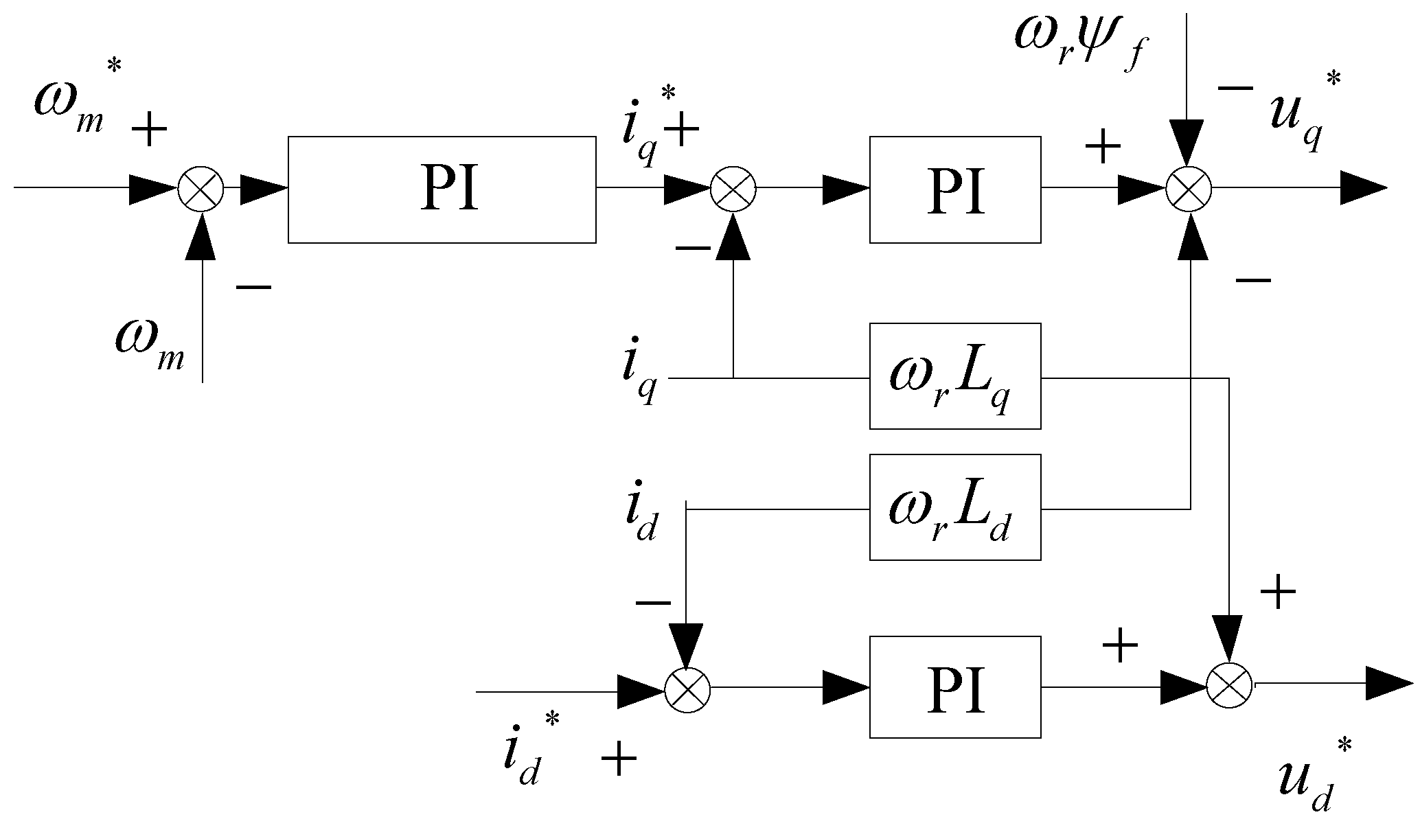
2.1. The Controller in Maximum Power Points Tracking Stage

The wind energy utilization coefficient C_p, tip-speed-ratio λ and pitch angle β have the following relationship [19]:

$$C_p(\mathsf{\lambda },\mathsf{\beta })=0.5173(\frac{116}{{\mathsf{\lambda }}_0}-0.4\mathsf{\beta }-5){\mathrm{e}}^{\frac{21}{{\mathsf{\lambda }}_0}}+0.0068\mathsf{\lambda }$$

(1)

where, λ₀ is a parameter related to the tip-speed-ratio λ; their relation is:

$$\frac{1}{{\mathsf{\lambda }}_0}=\frac{1}{\mathsf{\lambda }+0.08\mathsf{\beta }}-\frac{0.035}{{\mathsf{\beta }}^3+1}$$

(2)

When the wind speed remains stable and pitch angle β is fixed at a certain value, the wind energy utilization coefficient C_p of the wind turbine is only related to the value of the tip-speed-ratio λ, that is, only related to the rotating speed of the wind wheel, and when the speed reaches a certain value, the wind energy utilization coefficient has an optimal value C_pmax, corresponding to the best tip-speed-ratio λ_opt. At this time, the wind energy absorbed by the wind turbine reaches the maximum. When the pitch angle β increases, the maximum wind energy utilization coefficient C_pmax decreases, therefore, when the wind speed is below the rated value, the pitch angle is often adjusted to 0° (in practical engineering this is generally 3°). The reference speed of the generator is set based on the wind energy utilization coefficient formula and the real wind speed, so the wind power system can track the maximum wind energy utilization coefficient and output the maximum power by adjusting the generator speed [20]. The generator speed is usually controlled through the generator side converter, which generally adopts vector control based on rotor flux orientation [21]. The d-axis is oriented to the direction of the rotor flux, and q-axis is 90° ahead of d-axis.

The voltage equation of the stator of PMSG in synchronous rotating d–q coordinate system can be expressed as:

$$\{\begin{array}{l}{u}_d=R_s{i}_d+L_d\frac{\mathrm{d}{i}_d}{\mathrm{d}t}-{\mathsf{\omega }}_r{L}_q{i}_q\\ u_q=R_s{i}_q+L_q\frac{\mathrm{d}{i}_q}{\mathrm{d}t}+{\mathsf{\omega }}_r{L}_d{i}_d+{\mathsf{\omega }}_r{\mathsf{\psi }}_f\end{array}$$

(3)

where u_d, u_q, i_d and i_q are the d-axis and q-axis components of the stator’s terminal voltage and current; R_s is the resistance of stator winding; L_d and L_q are the d-axis and q-axis components of the stator’s inductance, respectively; ω_r is the electrical angular velocity of the generator; and ψ_f is flux linkage of the rotor.

When i_d is zero, the electromagnetic torque of PMSG, T_e, is:

$$T_e=\frac{3}{2}p({\mathsf{\psi }}_f{i}_q-(L_d-L_q)i_d{i}_q)=\frac{3}{2}p{\mathsf{\psi }}_f{i}_q$$

(4)

where, p is the pole pairs of generator.

PMDD wind turbines don’t have gearboxes. The wind wheel is directly connected with the generator rotor through the rotation shaft so that the generator rotor speed is equal to the speed of the wind wheel. The mathematical model of transmission system of PMDD wind turbines can be expressed as:

$$\frac{d{\mathsf{\omega }}_m}{dt}=\frac{1}{J}(T_m-T_e-B{\mathsf{\omega }}_m)$$

(5)

where, ω_m is mechanical angular velocity of rotor; J is moment of inertia of rotor; B is the damping coefficient; and T_m is the mechanical torque of the wind turbine. Equation (4) shows that the electromagnetic torque T_e can be controlled by controlling i_q. Equation (5) shows that the rotor speed ω_m can be further controlled by controlling T_e to realize the tracking control of maximum power.

Equation (3) indicates that the stator currents, i_d and i_q, are coupled with each other. Defining:

$$\{\begin{array}{l}{u_d}^{*}={\mathsf{\omega }}_r{L}_q{i}_q+u_d\\ {u_q}^{*}=-{\mathsf{\omega }}_r(L_d{i}_d+{\mathsf{\psi }}_f)+u_q\end{array}$$

(6)

Equation (6) is brought into Equation (3), after Laplace transform, and the following equation can be obtained:

$$\{\begin{array}{l}{i}_{sd}={u_d}^{*}/(L_{ds}s+R_s)\\ i_{sq}={u_q}^{*}/(L_{qs}s+R_s)\end{array}$$

(7)

where, s is Laplace operator.

Equation (7) shows that i_sd has a linear relationship with ${u_d}^{*}$, and i_sq has a linear relationship with ${u_q}^{*}$, what’s more, i_sd is independent of i_sq, so i_sd and i_sq can be controlled independently. The control diagram on the basis of above research is shown in Figure 1. The corresponding model based on Matlab/Simulink is shown in Figure 2.

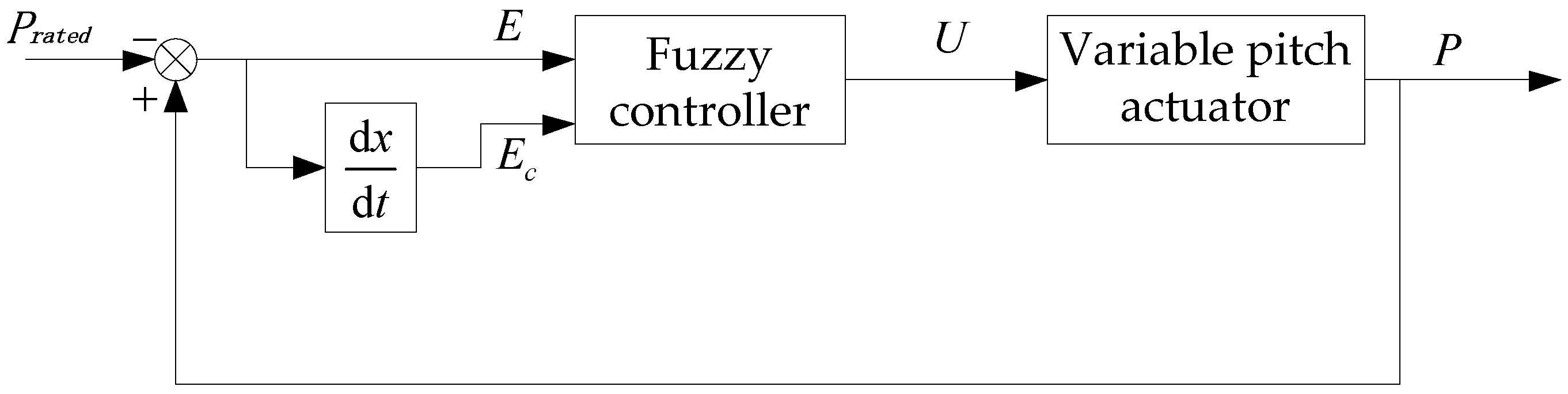
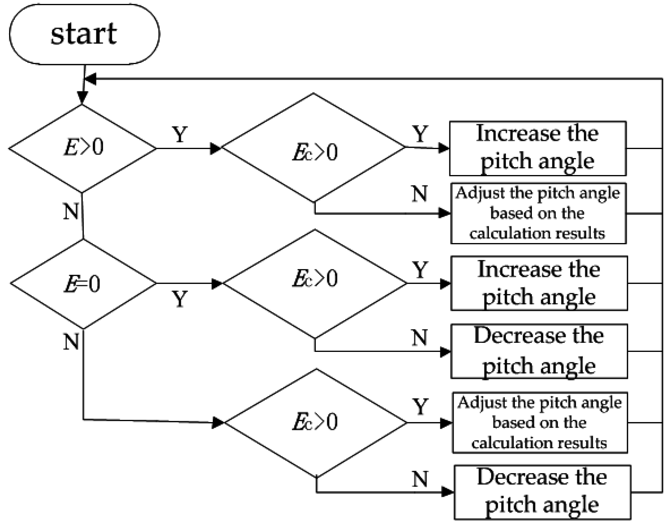
2.2. The Controller in the Constant Power Stage

In the constant power stage, the wind speed reaches or exceeds the rated value. It is necessary to limit the output power of the wind turbine in the vicinity of the rated power using the controller, because the mechanical structure and electrical characteristics of the wind turbine are limited and power network has requirements on the power quality generated by the wind turbine. In this condition, the pitch angle is usually adjusted to realize constant power control [22].

The real value of the output power is used as the feedback, while the rated power is the reference of the control in this paper. When the output power exceeds the rated value, the pitch angle increases to reduce wind energy absorption and the output power of the wind turbine; when the output power is less than the rated value, the pitch angle reduces to increase the wind energy absorption and the output power, which can make the generator output power remain in the vicinity of the rated power.

There are many methods to realize this control. For example, the regular PI method, which is simple and practical. PI control, however, doesn’t have parameter optimization functions. The parameters of a PI controller cannot be adjusted in response to changes in the external conditions, so the control algorithm can hardly accomplish the control target with high performance. A group of PI parameters which have been adjusted may provide a good control effect while the wind speed is near the rated value, however, the control would become poor if the wind speed changes. Fuzzy logic control is a basic modern control method that is often used. Its advantages include that it does not require complicated mathematical calculations and it can cope well with uncertainties and nonlinearities, and the effectiveness has been verified in many publications. Reference [8], is one of them, for example, where PI and fuzzy controllers were tested. Simulation results show the advantage of the proposed fuzzy control system, so a fuzzy control algorithm is adapted in this paper to realize constant power control.

For the fuzzy controller, the inputs are the error E and the error change rate E_c of the real value P of output power and the rated P_rated, and the output is the pitch angle U. A schematic diagram of fuzzy variable pitch controller is shown in Figure 3. The fuzzy pitch angle controller is designed according to the following steps:

(1) Fuzzification

The range of error E obtained from the simulation results of the system is (−25 kW, +25 kW), the selected domain of E is:

$$X=\left\{-6,-5,\cdots ,0,\cdots ,+5,+6\right\}$$

(8)

So the quantization factor of error E is K_e = 6/25000 = 0.00024.

The range of error change rate E_c obtained from the simulation results of the system is (−125 kW/s, +125 kW/s), the selected domain of E_c is:

$$Y=\left\{-6,-5,\cdots ,0,\cdots ,+5,+6\right\}$$

(9)

So the quantization factor of error change rate E_c is K_ec = 6/125000 = 0.000048.

The range of pitch angles U obtained from the simulation results of the system is (−12°, +12°), the selected domain of U is:

$$U=\left\{-6,-5,\cdots ,0,\cdots ,+5,+6\right\}$$

(10)

So the quantization factor of control quantity U is K_u = 12/6 = 2.

The membership functions of E, E_c and U are the triangle functions according to the experience.

(2) Fuzzy rules

Figure 4 shows the flow chart of the control logic, which is based on for writing fuzzy rules. When the power error is positive, the output power is greater than the rated power, so if the error change rate is positive, the error presents an increasing trend and the output power will continue to increase at that time, so the pitch angle should be increased in order to reduce the absorption of wind energy and the power output; when the error change rate is negative, the error presents a decreasing trend and the output power will continue to decrease at that time, so the pitch angle should be inferred based on the error and the error change rate.

When the error is 0, if the error change rate is positive, the power output presents a growth trend and may even exceed the rated power; at this time, the pitch angle should be increased; if the error change rate is negative, the pitch angle should be reduced.

When the error is negative, the output power is less than the rated power, so if the error change rate is positive, the output power presents a growth trend, and at this time, the pitch angle should be inferred based on the error and the error change rate avoiding power oscillations caused by excessive regulation; if the error change rate is negative, the output power presents a continuously decreasing trend, then, the pitch angle should be reduced to increase the wind energy absorption and make the output power achieve the rated value as soon as possible.

The selected language variables of E are:

$$\left\{\mathrm{NB},\mathrm{NM},\mathrm{NS},\mathrm{NZ},\mathrm{PZ},\mathrm{PS},\mathrm{PM},\mathrm{PB}\right\}$$

(11)

where NB: negative big; NM: negative medium; NS: negative small; NZ: negative zero; PZ: positive zero; PS: positive small; PM: positive medium; PB: positive big.

The selected language variables of E_c and U are:

$$\left\{\mathrm{NB},\mathrm{NM},\mathrm{NS},\mathrm{ZE},\mathrm{PS},\mathrm{PM},\mathrm{PB}\right\}$$

(12)

where, NE: zero. The control rules of the wind turbine can be extracted as shown in

Table 1. Fuzzy control rules. PB: positive big; PM: positive medium; PS: positive small; NE: zero; NS: negative small; NM: negative medium; NB: negative big; PZ: positive zero; NZ: negative zero.

		EC	PB	PM	PS	ZE	NS	NM	NB
	U
E
PB			PB	PB	PB	PB	PM	ZE	ZE
PM			PB	PB	PB	PB	PM	ZE	ZE
PS			PM	PM	PM	PM	ZE	NS	NS
PZ			PM	PM	PS	ZE	NS	NM	NM
NZ			PM	PM	PS	ZE	NS	NM	NM
NS			PS	PS	ZE	NM	NM	NM	NM
NM			ZE	ZE	NM	NB	NB	NB	NB
NB			ZE	ZE	NM	NB	NB	NB	NB

.

(3) Defuzzication

The Mamdani method is adopted for fuzzy reasoning in this paper, and the gravity method is adapted for defuzzication. The corresponding formula is:

$$u=\frac{{\displaystyle \sum U_i\mathsf{\mu }(U_i)}}{{\displaystyle \sum \mathsf{\mu }(U_i)}}$$

(13)

where, u is the exact amount after defuzzication; U_i is the fuzzy value of the output variable, and μ(U_i) is the corresponding value of the membership.

The Simulink model of the pitch angle controller is shown in Figure 5. When the wind speed is above the rated value, the error and the error change rate of the output power and the rated value are put into the fuzzy controller (scale factor K_e = 0.00024, K_ec = 0.000048), through the fuzzy inference, the output control variable U can be obtained, and then U is amplified appropriately by the quantization factor K_u = 2, and after defuzzication, the pitch angle is put into the pitch actuator to act on the wind turbine at last.

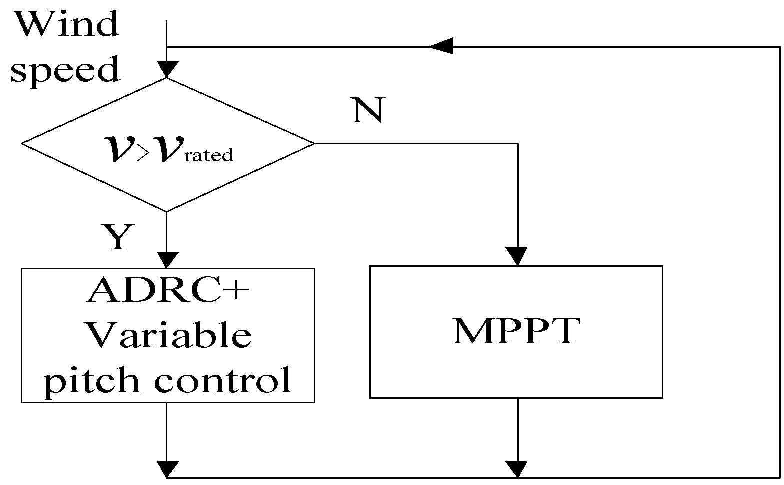
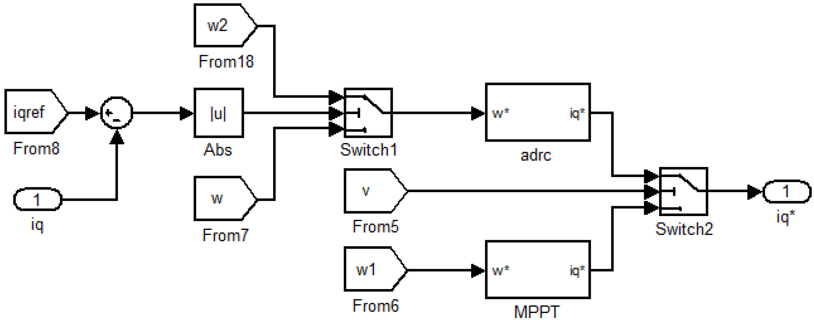
3. Sub-Controller Switching

When the wind speed is below the rated value, the maximum wind energy utilization coefficient of the wind turbine is tracked through the converter controller based on vector control. When the wind speed is higher than the rated value, the converter controller no longer tracks the maximum wind energy utilization coefficient, but rather the pitch angle controller based on the fuzzy algorithm begins to adjust the pitch angle to maintain the output power of the generator in the vicinity of the rated power.

When wind speed changes suddenly from below to above the rated value, the input of the converter controller changes, then changes in the d-axis and q-axis components of the current occur, which cause the abrupt change of the electromagnetic torque and output power. The d-axis and q-axis components of the current, electromagnetic torque and output power can be observed by simulation in Matlab/Simulink.

The simulation parameters of the wind turbine are: radius of wind turbine rotor, R = 38.7 m; rated wind speed, v = 12 m/s; air density, $\mathsf{\rho }$ = 1.225 kg/m³; the best tip-speed-ratio, λ_opt = 8; equivalent moment of inertia, J = 500 kg·m²; rated power is 2 MW; number of pole pairs of generator, p = 40; inductance L_d = L_q = 2.56 mH; stator resistance, R_s = 0.01 Ω; flux of permanent magnet, ψ_f = 1.67 Wb; viscosity coefficient of transmission, B = 0.005 N/(m/s).

An extreme case is used to demonstrate the response when sub-controller switching takes place. The wind speed change is shown in Figure 6. The wind speed is 8 m/s before t = 1 s and suddenly increases to a speed of 14 m/s at t = 1 s. The given range of wind speed contains two stages: below the rated and higher than the rated value, which can effectively simulate the changes of the system when the wind turbine continuously experiences two kinds of stages. The step changing wind speed is used to reflect the abrupt changing of wind speed and make the simulation results more typical.

Figure 7 and Figure 8 show the d-axis and q-axis components of the generator current. Figure 9 shows the simulation curve of the pitch angle. From the simulation results, it can be observed that the change in the q-axis current is far larger than that in the d-axis current, although through the adjustment of pitch angle, they are both finally tend to be stable, but the large overshoot will seriously affect the quality of the power.

Figure 10 and Figure 11 show the electromagnetic torque and output power of the simulation. From the results, the changes in the electromagnetic torque and the output power caused by the change in generator current can be easily observed. Therefore, it is necessary to design a switching controller to effectively restrain the abrupt changes of the generator current, make the transition of the system in the switching of sub-controllers smooth and reduce the impact and influence on the electrical equipment and power system as much as possible.

4. Design of the Active Disturbance Rejection Controller

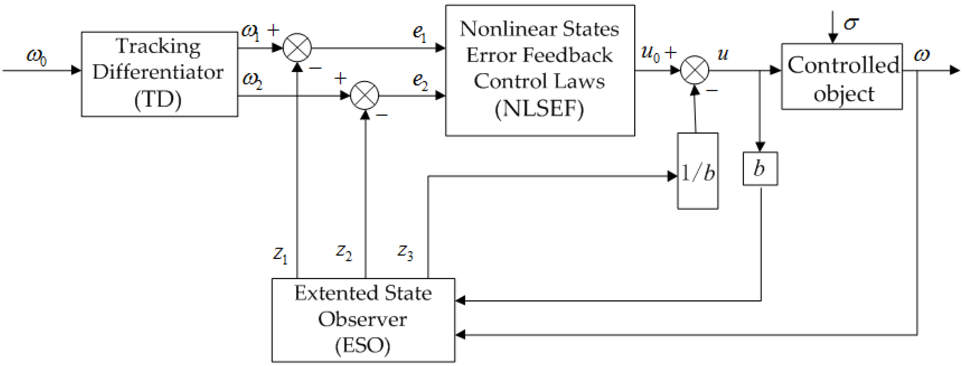
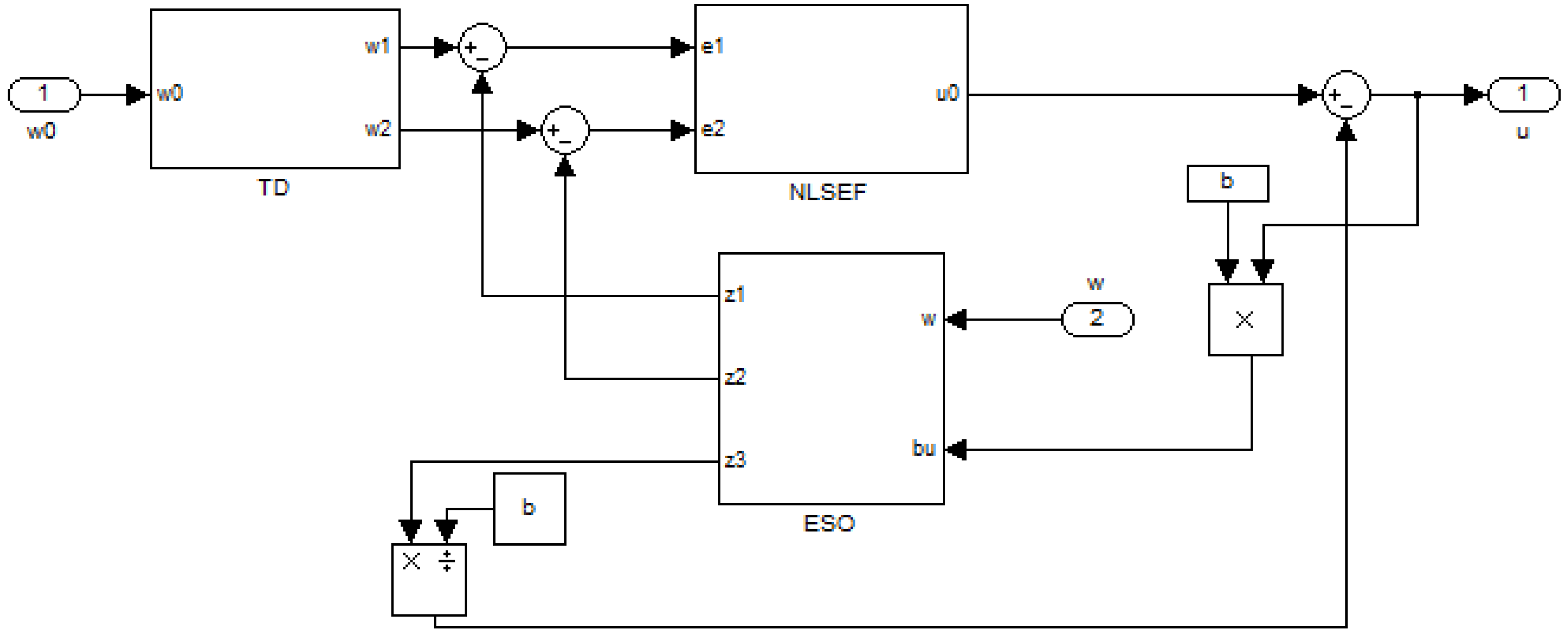
4.1. The Basic Principle of Active Disturbance Rejection Control

Based on the analysis of traditional control, Han used nonlinear effects to develop the functional aspects with better control performance and designed a new type of ADRC, which inherited the advantages and overcame the shortcomings of the traditional control, opened a new path for automatic control [23].

ADRC suppresses or eliminates the deviation based on monitoring the process, rather than relying on an accurate mathematical model of the system. It estimates and compensates the external disturbances of the system by using the deviation value of the given reference and the actual value as the control inputs to achieve the goal of ADRC. Because ADRC has the advantages of strong adaptability and robustness, it has been successfully applied in the field of temperature control, building intelligent system, missile guidance, manipulator control and so on [24].

Taking the second-order system as an example, the input is ω₀, the output is ω, the control variable is u, and the external disturbance is σ. Figure 12 shows the structure of the active disturbance rejection controller. It consists of a tracking differentiator (TD), extended state observer (ESO) and nonlinear state error feedback (NLSEF) control laws. The TD extracts the differential quantities of the controller input signal, and make it smooth; ESO turns a nonlinear system into an integral series structure, and uses the uncertain status of the system, the real-time variables of the internal and external disturbance as compensation inputs of the controller; the inputs of NLSEF are the errors of tracking signal, differential signal produced by TD and the state estimation signals of the controlled object produced by ESO, the output signal of NLSEF is the control component u₀ of the controlled object [25,26].

The active disturbance rejection algorithm for this second-order controlled system is:

(1) Produce tracking signal and differential signal

The tracking signal and the differential signal of the input signal are generated by TD, and the mathematical model is shown in the following:

$$\{\begin{array}{l}{\dot{\mathsf{\omega }}}_1{=\mathsf{\omega }}_1+h{\mathsf{\omega }}_2\hfill \\ {\dot{\mathsf{\omega }}}_2{=\mathsf{\omega }}_2+hfst({\mathsf{\omega }}_1-{\mathsf{\omega }}_0,{\mathsf{\omega }}_2,r,h_0)\hfill \end{array}$$

(14)

where ω₁, ω₂ are the tracking signal and differential signal of the input signal ω₀, h is the simulation step, r is speed factor, h₀ is the filtering factor, fst means a function. The expression of fst is as follows:

$$fst({\mathsf{\omega }}_1-{\mathsf{\omega }}_0,{\mathsf{\omega }}_2,r,h_0)=\{\begin{array}{c}\frac{-r\cdot a}{\mathsf{\delta }}\\ -r\cdot \mathrm{sign}\left(a\right)\end{array}\begin{array}{}\end{array}\begin{array}{c}\begin{array}{c}\left|a\right|\le \mathsf{\delta }\\ \left|a\right|>\mathsf{\delta }\end{array}\end{array}$$

(15)

where:

$$a=\{\begin{array}{c}{\mathsf{\omega }}_2+\frac{m}{h_0}\\ {\mathsf{\omega }}_2+0.5(a_0-\mathsf{\delta })\cdot \mathrm{sign}(m)\end{array}\begin{array}{c}\begin{array}{c}\left|m\right|\le {\mathsf{\delta }}_0\\ \left|m\right|>{\mathsf{\delta }}_0\end{array}\end{array}$$

(16)

$$\mathrm{sign}(m)=\{\begin{array}{c}1\\ 0\\ -1\end{array}\begin{array}{c}\begin{array}{c}m>0\\ m=0\\ m<0\end{array}\end{array}$$

(17)

Usually, the filtering factor h₀ is 3–10 times of the simulation step h. It is needed to determine the speed factor r according to the requirements of the rapidity of system transition or the differential signal. The relationship between r and the transition time T₀ is as follows:

$$r=\frac{4(x_1-x_0)}{{T_0}^2}$$

(18)

where, x₁ is the input ω₀ of TD, x₀ is the initial value of ω₀. Increasing the speed factor r will improve the transition speed of the system; reducing the speed factor r will decrease the transition speed. Usually r < 1, the smaller of r, the restraining overshoot effect is more obvious, but if r is too small, it will reduce the response speed of the system and increase the transition time.

(2) Estimate the state variables and total disturbance of the system

Estimating the state variables and total disturbance of the system is performed by ESO. The mathematical model of ESO is shown by:

$$\{\begin{array}{l}{e}_0=z_1-\mathsf{\omega }\hfill \\ {\dot{z}}_1=z_1+h(z_2-{\mathsf{\beta }}_1{e}_0)\hfill \\ {\dot{z}}_2=z_2+h[z_3-{\mathsf{\beta }}_{2}fal(e_0,{\mathsf{\alpha }}_1,{\mathsf{\delta }}_0)+bu]\hfill \\ {\dot{z}}_3=z_3-h{\mathsf{\beta }}_{3}fal(e_0,{\alpha }_2,{\mathsf{\delta }}_0)\hfill \end{array}$$

(19)

where, z₁ estimates the output ω, z₂ estimates the differential of ω, z₃ estimates the total disturbance of the system, fal means a function. The expression of fal(e,α, ${\mathsf{\delta }}_{*}$) is as follows:

$$fal(e,\mathsf{\alpha },{\mathsf{\delta }}_{\ast })=\{\begin{array}{c}{\left|e\right|}^{\mathsf{\alpha }}\mathrm{sign}(e) \left|e\right|>{\mathsf{\delta }}_{*}\ge 0\\ \frac{e}{{\mathsf{\delta }}_{\ast }^{1-\mathsf{\alpha }}} \left|e\right|\le {\mathsf{\delta }}_{\ast }\end{array}$$

(20)

Selecting the appropriate parameters α₁, α₂, δ₀, b, β₁, β₂, β₃, ESO can estimate the state variables and the total disturbance of the system very well.

Usually, α₁ = 0.25, α₂ = 0.5. The value of parameter δ₀ is related to the nonlinear performance of active disturbance rejection controller, when the value is too small, the control effect may be trembled; when the value is too large, the active disturbance rejection controller may lose the nonlinear characteristics and work in the linear region.

Tuning the parameters β₁, β₂, β₃ will affect the stability of ESO. Usually, parameter β₁ is tuned according to the simulation step h, β₁ = 1/h, β₂ and β₃ depend on β₁:

$$\{\begin{array}{c}{\mathsf{\beta }}_2=\frac{{\mathsf{\beta }}_1}{h}\\ {\mathsf{\beta }}_3=\frac{{\mathsf{\beta }}_2}{h}\end{array}$$

(21)

where b is the coefficient of the control input.

(3) Produce control quantity

The inputs of NLSEF are the errors of ω₁ & z₁ and ω₂ & z₂, the control variable of the controlled object is u. The mathematical equations are shown as:

$$\{\begin{array}{l}{e}_1={\mathsf{\omega }}_1-z_1\hfill \\ e_2={\mathsf{\omega }}_2-z_2\hfill \\ u_0={\mathsf{\beta }}_{4}fal(e_1,{\mathsf{\alpha }}_3,{\mathsf{\delta }}_1)+{\mathsf{\beta }}_{5}fal(e_2,{\mathsf{\alpha }}_4,{\mathsf{\delta }}_1)\hfill \\ u=u_0-\frac{z_3}{b}\hfill \end{array}$$

(22)

Selecting the appropriate parameters α₃, α₄, δ₁, β₄, β₅ and b, NLSEF can achieve the nonlinear configuration and generate the control component u₀, after superposing the compensation component of the object model and the external disturbance, the appropriate control variable u can be gotten. The parameter β₄ is similar to the proportion parameter K_p in the the PID controller, when the overshoot is too much, β₄ should be reduced. The parameter β₅ is similar to the integral parameter K_i in the PID controller, increasing β₅ can reduce the adjusting time, but it can also cause the increasing of overshoot and oscillation amplitude of the system. Parameter δ₁ is similar to parameter δ₀.

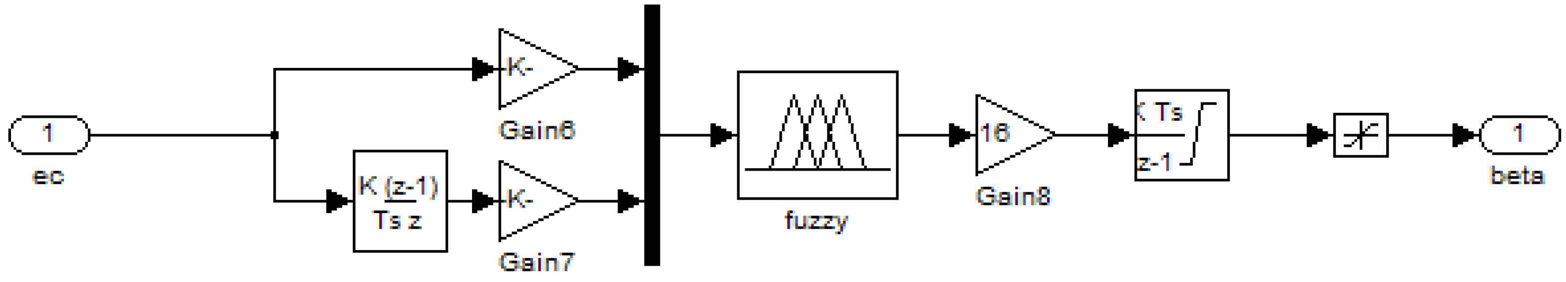
4.2. Design of Active Disturbance Rejection Controller

Active disturbance rejection controller built in MATLAB/Simulink is shown in Figure 13, the input is the reference generator speed ω₀ and the output u is q-axis reference current, which acts on the converter controller to suppress the q-axis current.

Figure 14 is the switching process of the proposed system. When the wind speed is below the rated value, the MPPT module is executed, its input is the given reference generator speed based on the best tip-speed-ratio λ_opt (λ_opt = ω_ref R/v, where R is the radius of the wind turbine rotor, v is the wind speed); when the wind speed is above the rated value, the ADRC module is executed and the q-axis current is determined whether it tends to be the reference current. If q-axis current tends to be the reference current, the real-time generator speed is input to ADRC module; if the q-axis current deviates from the reference current, the given reference speed based on the wind speed and pitch angle is input to ADRC module. Figure 15 is the corresponding switching Simulink model of the system.

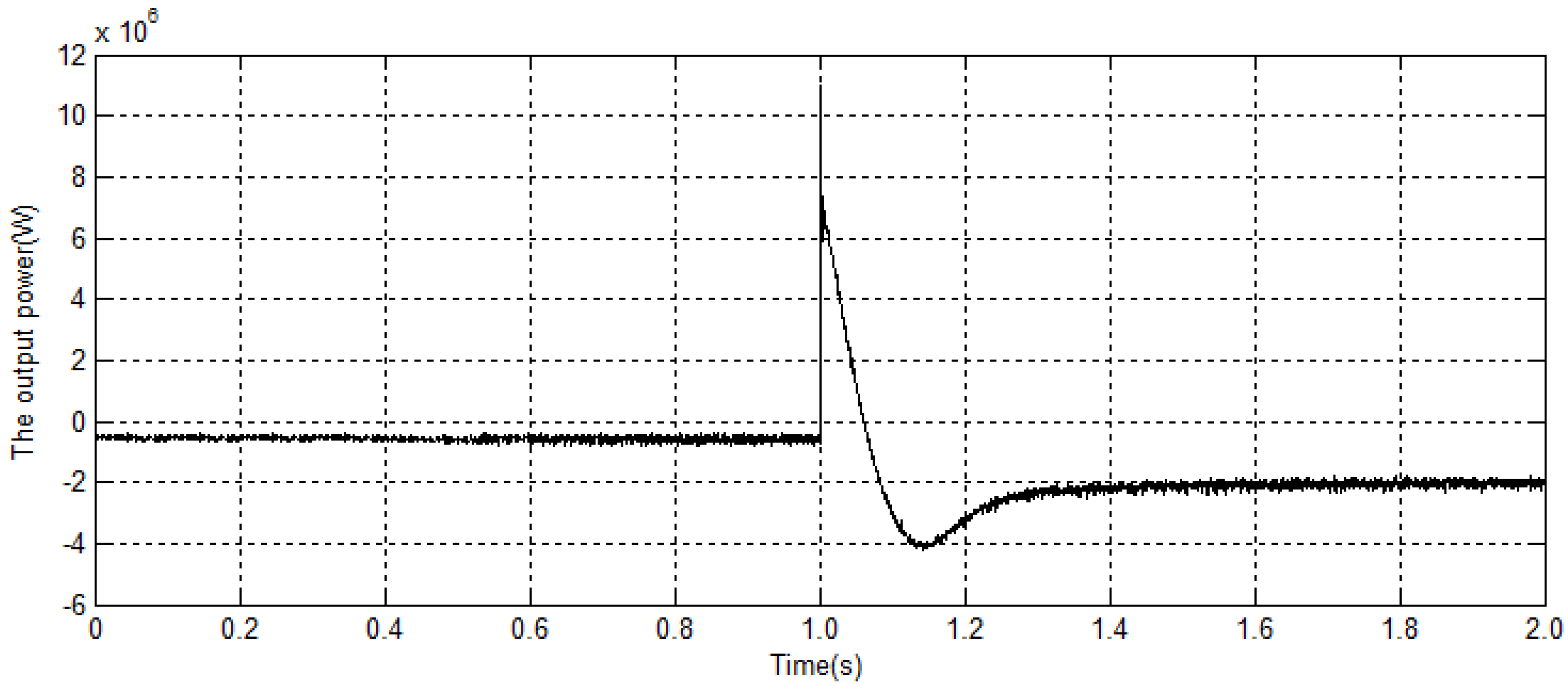
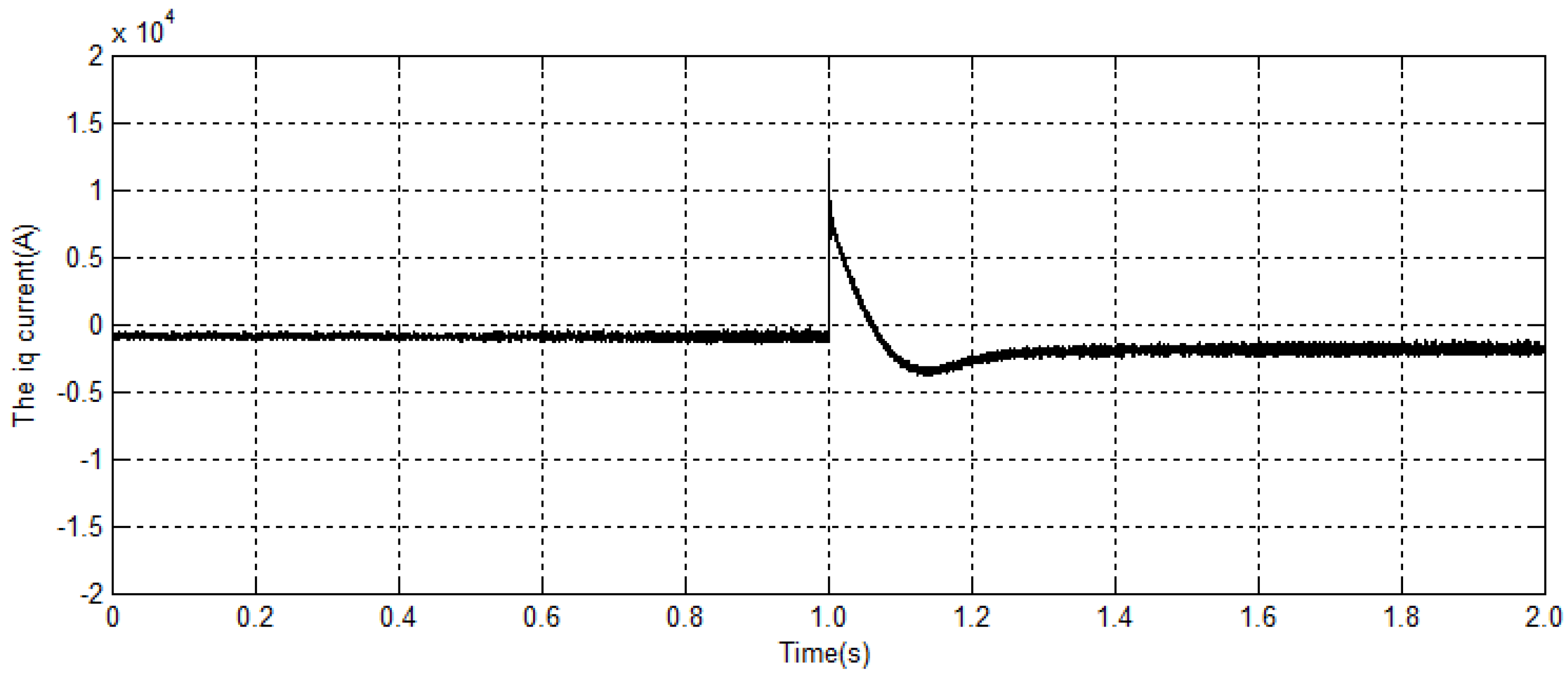
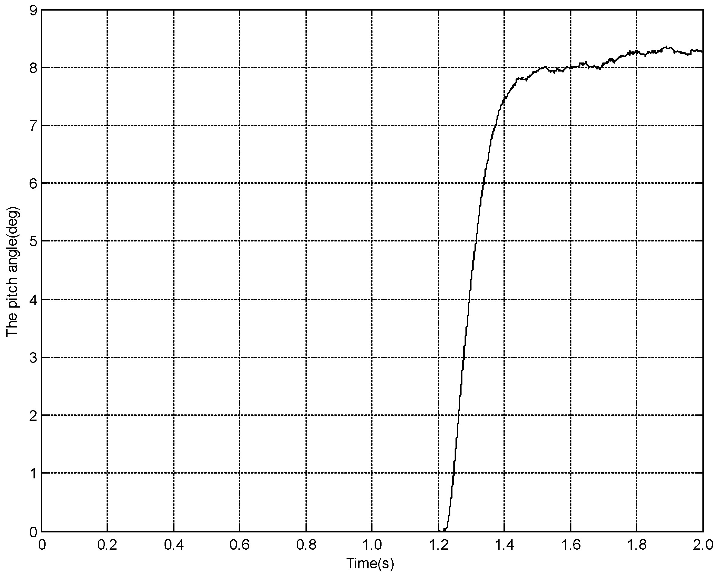
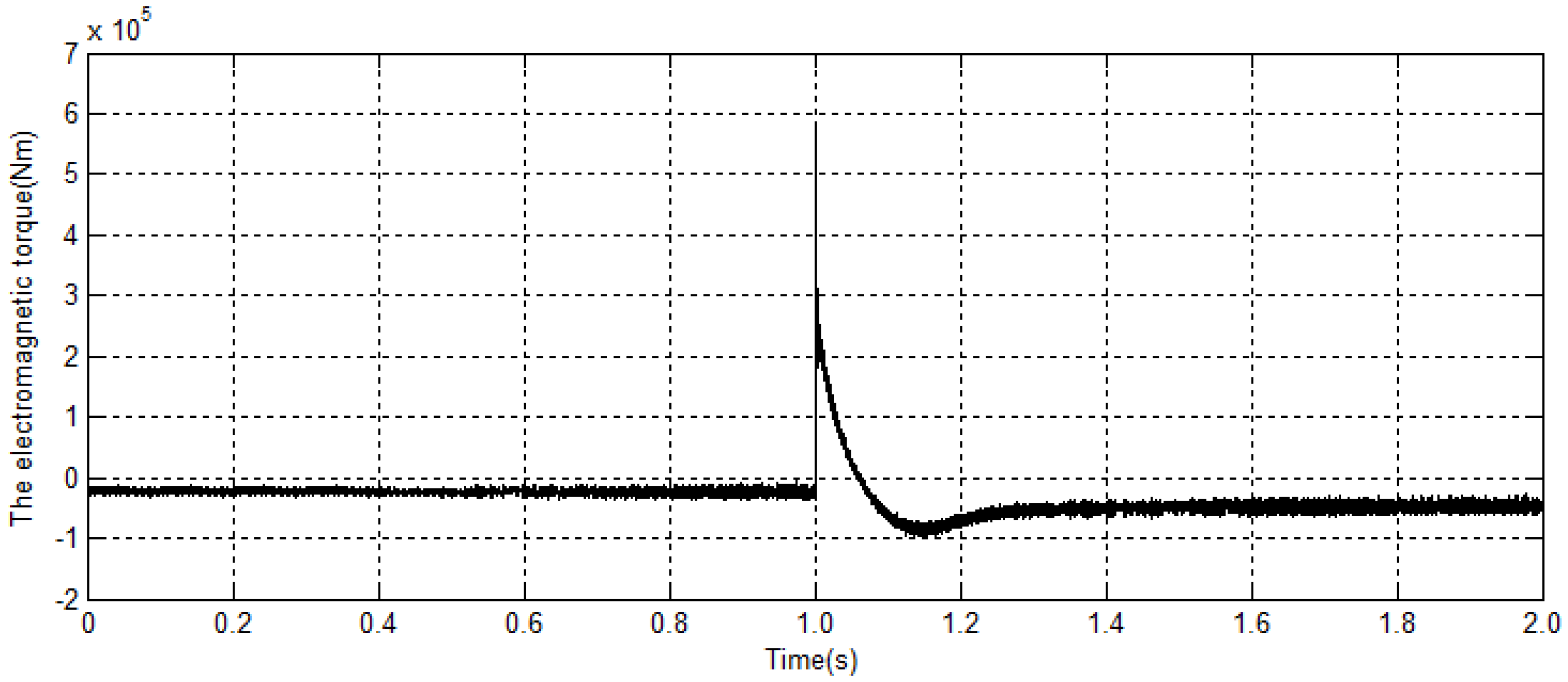
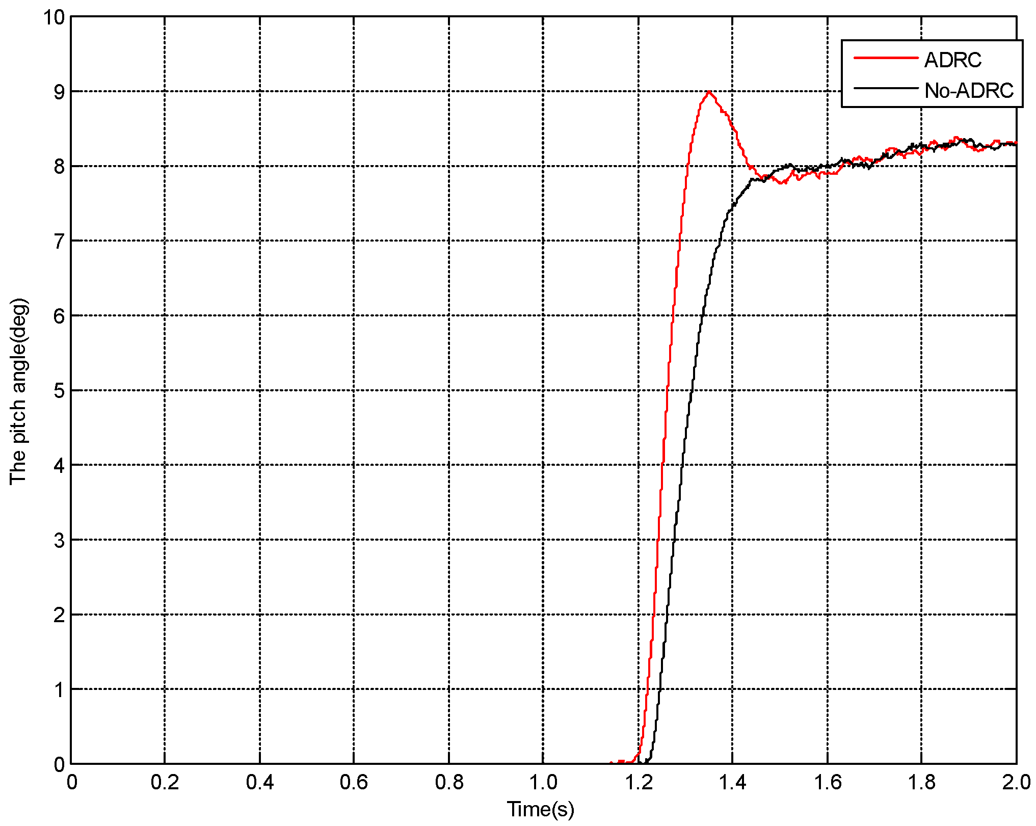
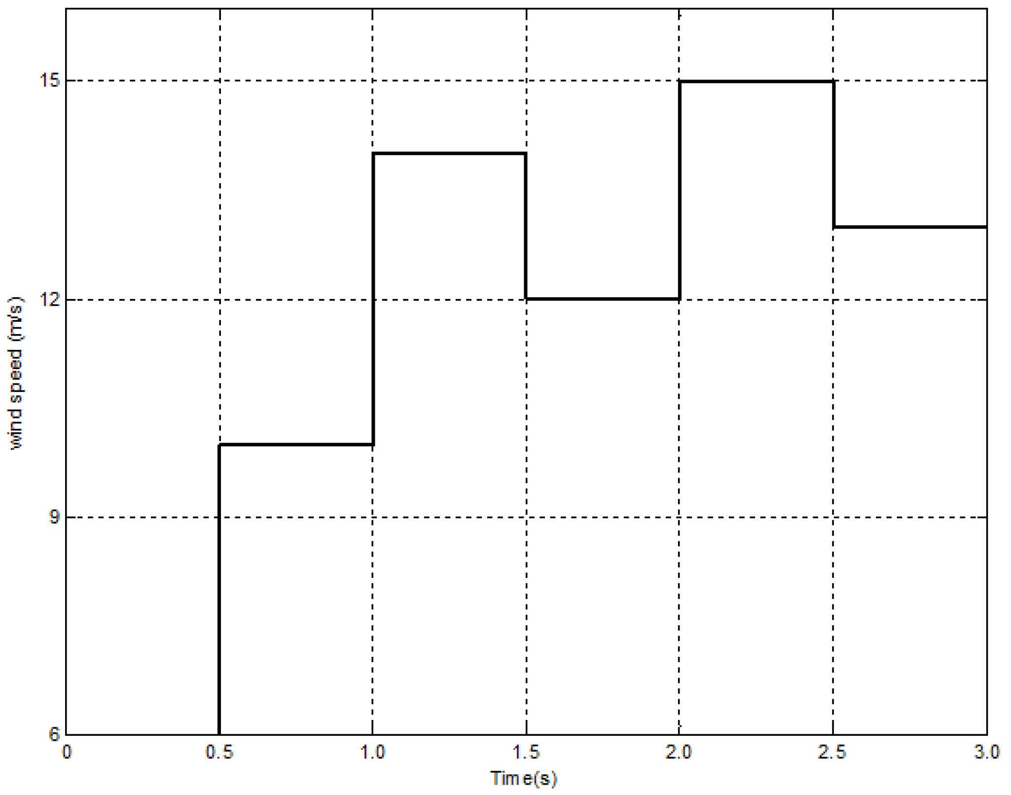
5. Simulation Analysis

The parameters of ADRC are adjusted by first separately tuning the parameters of TD and ESO to achieve a relatively satisfactory performance; then combining the parameter adjustment of NLSEF to ensure ADRC to achieve a more satisfactory performance. Specifically: (1) determine the simulation step h, then adjust parameter r, the larger r is, the shorter the transition process, the weaker the softening effect, just as shown in Equation (18); (2) let α₁ = 0.25, α₂ = 0.5, β₁ = 1/h, determine β₂, β₃ according to Equation (21), adjust the value of δ₀ with the control effect; (3) as described above, regulate β₄ according to the overshoot and tune β₅ according to regulation time. The adjustment of δ₁ is same as δ₀. In this way, the parameters of the active disturbance rejection controller are selected as follows: h = 0.05, r = 0.1, h₀ = 0.15, α₁ = 0.25, α₂ = 0.5, α₃ = 0.25, α₄ = 0.5, δ₀ = 0.01, δ₁ = 0.001, b = 2261.4, β₁ = 20, β₂ = 400, β₃ = 8000, β₄ = 20, β₅ = 100.

Still simulating at the same wind speed as shown in Figure 6, the q-axis current is shown in Figure 16, for contrast the corresponding curve of direct switching is also shown in the figure. It can be observed from the figure that ADRC controller can restrain the q-axis current mutation. The simulation results are shown in

Table 2. Simulation results of q-axis current.

Controller	Regulating Time	Overshoot	Steady-State Error
No-ADRC	0.33 s	99.98%	22.00%
ADRC	0.45 s	25.00%	16.88%

.

Figure 17 is the corresponding curves of generator electromagnetic torque, it can be observed from the figure that ADRC controller can restrain the mutation. The simulation results are shown in

Table 3. Simulation results of electromagnetic torque.

Controller	Regulating Time	Overshoot	Steady-State Error
No-ADRC	0.27 s	152.27%	25.42%
ADRC	0.31 s	61.82%	11.86%

.

Figure 18 shows the simulation curves of the output power. It can be seen from the figure that the mutation of the output power caused by the sudden change of the conditions is suppressed under the ADRC controller. The simulation results are shown in

Table 4. Simulation results of output power.

Controller	Regulating Time	Overshoot
No-ADRC	0.33 s	107.50%
ADRC	0.46 s	40.28%

.

Figure 19 shows the simulation curves of the pitch angle. The simulation results are shown in

Table 5. Simulation results of pitch angle.

Controller	Regulating Time	Overshoot
No-ADRC	0.47 s	0.66%
ADRC	0.54 s	8.31%

. It can be seen that the mutations of the pith angle caused by the sudden change are both within 8.5%. This is acceptable.

Figure 20 shows simulation curve of the wind speed. Figure 21, Figure 22, Figure 23 and Figure 24 are simulation results under the wind speed according to Figure 20.

Through analyzing the simulation results, it can be concluded that the ADRC controller can meet the requirements of switching without disturbance and restrain the fluctuation of output power through controlling the q-axis current when the wind turbine running from MPPT stage to the constant power stage.

6. Conclusions

A simulation model of PMDD wind turbine has been established using MATLAB/Simulink in this paper; the PI sub-controller in the MPPT stage when wind speed is below the rated value is designed; a fuzzy pitch angle sub-controller in the constant power stage when the wind speed is higher than the rated value has been described carefully. The ADRC technique is adopted to solve the output power fluctuation of wind turbines in the sub-controllers’ switching process. The undisturbed switching of the system is realized basically, the abrupt change of the output power in the switching transition is greatly reduced and the system’s performance is improved.

This paper focuses only on the switching from the MPPT stage to the constant power stage, but in practice, the running of the PMDD wind power generation system can be divided into several states including starting, MPPT, constant power and so on, so there is potential to extend the study to other switching processes. Meanwhile, the actual operation of the system may drop in grid voltage or load imbalance, but the present paper only considers the normal situation. Moreover, the ADRC also needs time to run and it might require new hardware to be installed in practical implementation. As a result, when implementing the controller in reality in a microprocessor, the calculation speed of the microprocessor needs to be higher in order to complete the complex arithmetic operations during the wind speed sampling interval. Therefore, further research will be pursued on practical application.

References

1. Xu, T. Statistics on global wind power installed capacity in 2015. Wind Energy Ind. 2016, 2016, 51–56. [Google Scholar]
2. European Wind Energy Association. Pure Power: Wind Energy Targets for 2020 and 2030, 2009 Update. Available online: http://www.ewea.org/fileadmin/ewea_documents/documents/publications/reports/ Pure_power_Full_Report.pdf (accessed on 31 July 2015).
3. The US Department of Energy (US DoE). Chapter 4: The Wind Vision Roadmap: A Pathway Forward in Wind Vision: A New Era for Wind Power in the United States. Available online: http://www.energy.gov/ sites/prod/files/wv_chapter4_the_wind_vision_roadmap.pdf (accessed on 20 March 2016).
4. China May Have 500 GW of Wind Parks in 2030—Study (21 October 2014). Available online: http://renewables.seenews.com/news/china-may-have-500-gw-of-wind-parks-in-2030-study-444069 (accessed on 20 March 2016).
5. Gu, F. Power Control of Wind Farm Based on Doubly-fed Generators. Master’s Thesis, Shandong University, Jinan, China, April 2009. [Google Scholar]
6. Xiao, Y.; Zhang, T.; Ding, Z.; Li, C. The Study of Fuzzy Proportional Integral Controllers Based on Improved Particle Swarm Optimization for Permanent Magnet Direct Drive Wind Turbine Converters. Energies 2016, 9, 343. [Google Scholar] [CrossRef]
7. Tiang, T.L.; Ishak, D. Novel MPPT control in permanent magnet synchronous generator system for battery energy storage. In Proceedings of the 2nd International Conference on Mechanical and Aerospace Engineering, Bangkok, Thailand, 29–31 July 2011; pp. 5179–5183.
8. Amine, B.M.; Souhila, Z.; Tayeb, A.; Ahmed, M. Adaptive fuzzy logic control of wind turbine emulator. Int. J. Power Electron. Drive Syst. 2014, 4, 233–240. [Google Scholar]
9. Minh, H.Q.; Cuong, N.C.; Chau, T.N. A fuzzy-logic based MPPT method for stand-alone wind turbine system. Am. J. Eng. Res. 2014, 3, 177–184. [Google Scholar]
10. Yin, X.X.; Lin, Y.G.; Li, W.; Gu, Y.J.; Lei, P.F.; Liu, H.W. Sliding mode voltage control strategy for capturing maximum wind energy based on fuzzy logic control. Int. J. Emerg. Electr. Power Syst. 2015, 70, 45–51. [Google Scholar] [CrossRef]
11. Babu, N.R.; Arulmozhivarman, P. Wind energy conversion systems—A technical review. J. Eng. Sci. Technol. 2013, 8, 493–507. [Google Scholar]
12. Salazar, J.; Tadeo, F.; Witheephanich, K.; Hayes, M.; de Prada, C. Control for a variable speed wind turbine equipped with a permanent magnet synchronous generator (PMSG). In Proceedings of the 3rd International Conference on Sustainability in Energy and Buildings (SEB’11), Marseilles, France, 1–3 June 2011; pp. 151–168.
13. Van Tan, L.; Nguyen, T.H.; Lee, D.-C. Advanced Pitch Angle Control Based on Fuzzy Logic for Variable-Speed Wind Turbine Systems. IEEE Trans. Energy Convers. 2015, 30, 578–587. [Google Scholar] [CrossRef]
14. Xiao, Y.; Huo, W.; Nan, G. Study of Variable Pitch Control for Direct-drive Permanent Magnet Wind Turbines Based on Fuzzy Logic Algorithm. J. Inf. Comput. Sci. 2015, 12, 2849–2856. [Google Scholar] [CrossRef]
15. Liao, Q.; Qiu, X.-Y.; Jiang, R.-Z. Variable pitch control of wind turbine based on RBF neural network. In Proceedings of the 2014 International Conference on Power System Technology (POWERCON), Chengdu, China, 20–22 October 2014.
16. Wang, X.; Zhu, W.; Qin, B.; Li, P. Sliding mode control of pitch angle for direct driven PM wind turbine. In Proceedings of the 26th Chinese Control and Decision Conference (CCDC), Changsha, China, 31 May–2 June 2014.
17. Mansour, M.; Mansouri, M.N.; Mimouni, M.F. Study of performance of a variable-speed wind turbine with pitch control based on a permanent magnet synchronous generator. In Proceedings of the International Multi-Conference on Systems, Signals and Devices (SSD’11), Sousse, Tunisia, 22–25 March 2011. [CrossRef]
18. Lee, S.-H.; Joo, Y.; Back, J.; Seo, J.-H.; Choy, I. Sliding mode controller for torque and pitch control of PMSG wind power systems. J. Power Electron. 2011, 11, 342–349. [Google Scholar] [CrossRef]
19. Kim, H.W.; Kin, S.S.; Ko, H.S. Modeling and control of PMSG-based variable-speed wind turbine. Electr. Power Syst. Res. 2010, 80, 46–52. [Google Scholar] [CrossRef]
20. Ren, Y.; An, Q. Flexible Grid Connected Operation and Control of Doubly Fed Wind Power Generation Unit, 1st ed.; China Machine Press: Beijing, China, 2011; pp. 120–144. [Google Scholar]
21. Chi, W.; Shi, Q.; Chen, H. Control strategy study of direct-driven wind-power system with PMSG based on back-to-back PWM converter. J. Mech. Electr. Eng. 2012, 29, 434–438. [Google Scholar]
22. Wang, S.; Li, Z. Adaptive PI optimization control for variable-pitch wind turbines. Acta Energiae Solaris Sin. 2013, 34, 1579–1586. [Google Scholar]
23. Han, J. Auto-disturbances-rejection Controller and It’s Applications. Control Decis. 1998, 13, 1579–1586. [Google Scholar]
24. Sun, K.; Zhao, Y.; Shu, Q. A position sensorless vector control system of permanent magnet synchronous motor based on active-disturbance rejection controller. In Proceedings of the IEEE International Conference on Mechatronics and Automation, Changchun, China, 9–12 August 2009.
25. Han, J. From PID technique to active disturbances rejection control technique. Control Eng. China 2002, 9, 13–18. [Google Scholar]
26. Huang, Y.; Zhang, W. Development of active disturbance rejection controller. Control Theory Appl. 2002, 19, 484–492. [Google Scholar]
Figure 1. Control diagram of the generator side converter.
Energies 09 00793 g001
Figure 2. Simulink model of the generator side converter.
Energies 09 00793 g002
Figure 3. Schematic diagram of the fuzzy variable pitch controller.
Energies 09 00793 g003
Figure 4. Flow chart of the control logic.
Energies 09 00793 g004
Figure 5. The Simulink model of the pitch angle controller.
Energies 09 00793 g005
Figure 6. Wind speed simulation curve.
Energies 09 00793 g006
Figure 7. The current simulation curve of the d-axis.
Energies 09 00793 g007
Figure 8. The current simulation curve of the q-axis.
Energies 09 00793 g008
Figure 9. The simulation curve of the pitch angle.
Energies 09 00793 g009
Figure 10. Simulation curve of electromagnetic torque.
Energies 09 00793 g010
Figure 11. Simulation curve of output power.
Energies 09 00793 g011
Figure 12. Structure of the active disturbance rejection controller.
Energies 09 00793 g012
Figure 13. The Simulink model of the active disturbance rejection controller.
Energies 09 00793 g013
Figure 14. The switching process of the proposed system.
Energies 09 00793 g014
Figure 15. The switching Simulink model.
Energies 09 00793 g015
Figure 16. Simulation curve of the q-axis current.
Energies 09 00793 g016
Figure 17. Simulation curve of the electromagnetic torque.
Energies 09 00793 g017
Figure 18. Simulation curve of the output power.
Energies 09 00793 g018
Figure 19. Simulation curve of pitch angle.
Energies 09 00793 g019
Figure 20. Simulation curve of the wind speed.
Energies 09 00793 g020
Figure 21. Simulation curve of the q-axis current.
Energies 09 00793 g021
Figure 22. Simulation curve of the electromagnetic torque.
Energies 09 00793 g022
Figure 23. Simulation curve of the output power.
Energies 09 00793 g023
Figure 24. Simulation curve of pitch angle.
Energies 09 00793 g024