A New Approach to Obtain Synthetic Wind Power Forecasts for Integration Studies

Abstract

When performing wind integration studies, synthetic wind power forecasts are key elements. Historically, data from operational forecasting systems have been used sparsely, likely due to the high costs involved. Purely statistical methods for simulating wind power forecasts are more common, but have problems mimicking all relevant aspects of actual forecasts. Consequently, a new approach to obtain wind power forecasts for integration studies is proposed, relying on long time series of freely and globally available reforecasts. In order to produce synthetic forecasts with similar properties as operational ditto, some processing (noise addition and error reduction) is necessary. Validations with measurements from Belgium and Sweden show that the method is adequate; and distributions, correlations, autocorrelations and power spectral densities of forecast errors correspond well. Furthermore, abrupt changes when forecasts are updated and the existence of level and phase errors are reproduced. The influence from terrain complexity on error magnitude is promising, but more data is necessary for a proper validation.

1. Introduction

For low wind power penetration rates, the uncertainty in the net load (load minus wind generation) is dominated by load uncertainty. However, wind power forecasts errors (FEs) become increasingly important for higher penetration levels, and it is therefore not surprising that wind power forecasting is a very active research field. Traditionally, research focus has been on improving the performance of point forecasts [1], but recently a lot of attention has been drawn to probabilistic forecasts, providing the user with prediction intervals. The anticipated uncertainty, which depend on, for instance, forecasts horizon and meteorological conditions, can be valuable for reserve quantification, unit commitment, power system planning and design of trading strategies [2]. Commonly, probabilistic forecasts are obtained from ensemble numerical weather prediction (NWP) models where several members are produced by perturbing the initial conditions. Different NWP models can also be combined, both to improve point forecasts and to get information on prediction intervals [3].

Because of its importance for the operation of the power system, wind power uncertainty needs to be accounted for in wind integration studies. According to IEA (International Energy Agency) wind [4], forecast data are needed for studies of unit commitment and economic dispatch including reserve requirements. For load flow analyses, forecast data will be needed in the future. When analysing scenarios of future wind power deployment, synthetic forecasts thus need to be obtained in one way or another. If time series are desired (i.e., not only information on FE distributions) this can in principle be obtained in three ways: by linear scaling of historical forecasts, by statistical models or by using NWP models, possibly in combination with some statistical post-processing.

A review of wind integration studies from 2007 to 2016, both journal papers and reports from e.g., system operators, revealed that NWP based forecasts were rarely used [5,6,7], most likely due to high monetary and computational costs. Purely statistical approaches such as time series models, persistence or assumed FE distributions were however common [8,9,10,11,12,13,14,15,16,17,18]. Many authors did not consider FEs directly [19,20,21,22,23,24,25,26,27], although sometimes mentioned their importance.

Actual forecast errors have several characteristics, some of which make them challenging to simulate with statistical methods, e.g.,

• Increase with forecast horizon and terrain complexity [28];
• The MW (megawatt) errors depend on the wind speed since the power curve is non-linear;
• The m/s (metre per second) errors depend on the wind speed [29], although to a less extent than the MW error;
• The errors can be level or phase errors [30]. The latter are short-lived but can be very large;
• The FEs are autocorrelated;
• The distribution is often skewed and heavy-tailed rather than normal [31];
• The errors are correlated between sites. The correlation depends primarily on distance and forecast horizon [30], but other factors may also be important;
• Errors from consecutive forecasts are not independent. If, for example, the five day-ahead (D + 5) forecast issued a certain day is too conservative (forecast < generation), and then it is likely that the D + 4 forecast issued the following day is also too conservative.

Additional dependencies possibly exist between the magnitude/correlation of FEs and meteorological conditions such as wind direction, atmospheric stability, seasonal and diurnal patterns, etc. As an example, if the wind blows from wind farm A towards farm B, it is likely that a phase error at A is followed by a phase error at B. Taken together, there are thus several reasons to believe that NWP based synthetic forecasts can be more realistic than synthetic forecasts from purely statistical models.

Our rationale for developing the model described in this paper was to be able to produce realistic day-ahead up to week-ahead forecasts for studies of large scale wind power integration in the Nordic power system. Balancing load and wind power generation in the Nordic countries is essentially a matter of hydropower dispatch planning, i.e., making sure that water and plant capacities are available when needed and that the system is utilized efficiently. With the majority of the hydropower plants located in fairly long and complex river systems, coupled hydraulically to each other and to the natural water inflow, the dispatch is planned and re-planned daily using a combination of optimization tools and forecasts stretching days, weeks, months and years ahead. Although the hydropower production can be ramped up and down quickly, transferring the large amounts of water required to balance wind power variations on the synoptic scale may take several days. The hydrological couplings makes it necessary to use forecast trajectories and not only statistical distributions.

Several decades of temporally consistent (by consistent, we mean that the quality of the forecasts does not change substantially over the years) time series for assumed future scenarios of wind farms are thus desired. Originally, our plan was to adapt and improve earlier statistical models for simulation of wind forecasts [32,33,34] so that these became more suitable for longer forecast horizons and captured more of the characteristics of actual forecasts. Because of the challenges involved, we however started looking for alternative strategies. Over the last years, modelling of (national) wind power generation from relatively coarse reanalysis datasets has become more popular and proven successful [35,36]. Maybe global, coarse wind speed forecasts could be used in a similar manner for generating synthetic wind power forecasts for a country?

In this paper, a new method for producing synthetic wind power forecasts is proposed. For validation, the output from the model is compared to actual forecasts and FEs from individual farms as well as for a whole country. The remainder of the paper is structured as follows. First, the data used (measurements and meteorological datasets) are described. The methodology is described in Section 3 and results are given in Section 4. The paper is concluded with a discussion section and some conclusions.

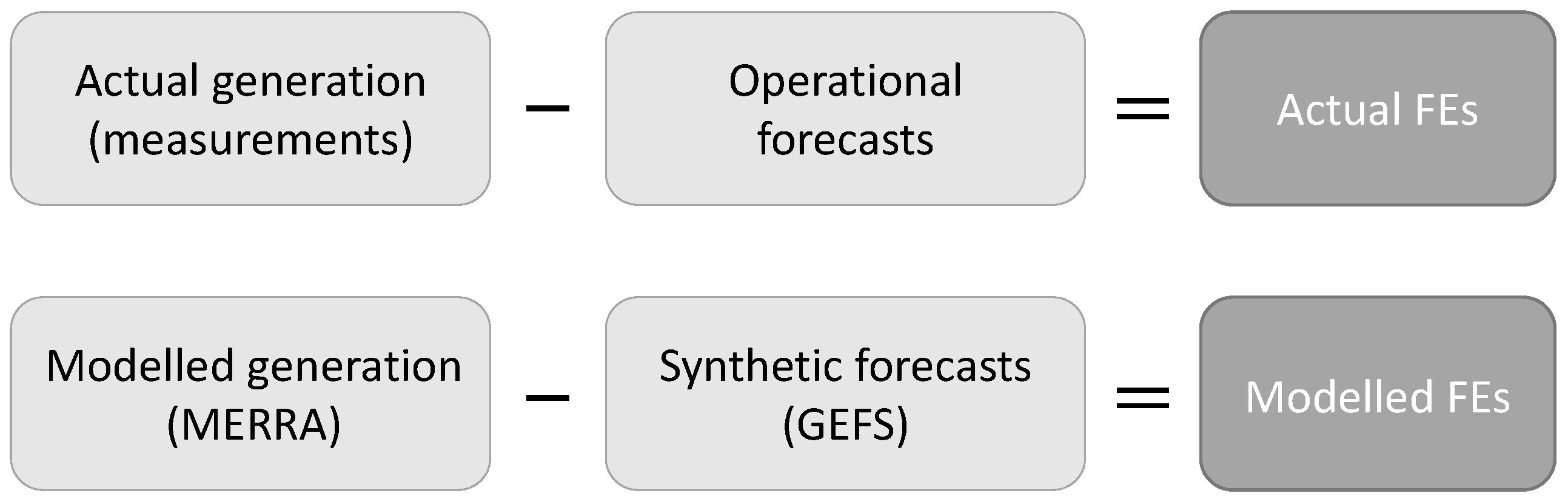
For the sake of clarity, this section is concluded with Figure 1, showing how actual and modelled wind power generation, forecasts and forecast errors are related and denoted. In the upper row, actual variables (measurements and operational forecasts) are presented. These are sometimes collectively referred to as “measurements”. In the lower row, the modelled variables are given. The differences between the modelled generation and the synthetic forecasts are denoted “modelled FEs” although these are not modelled directly. In principle, it is desirable that the modelled generation is similar to the actual generation, that the synthetic forecasts are similar to operational forecasts and that modelled and actual FEs are similar. The focus of this paper is mostly on the latter. These relations are desirable for the model validation phase. When producing forecast time series for future wind power scenarios, it is reasonable to assume that the forecasting systems will have improved. The model parameters should thus be tuned to give lower errors.

2. Data

For evaluating the similarity of the synthetic and operational forecasts as well as the corresponding FEs, measurements for three farms in Sweden and for aggregated generation in Belgium were obtained. The Swedish data consist of 12–18 months of day-ahead (D + 1) forecasts issued every day around noon, i.e., a forecast horizon of 12–35 h. The Belgian transmission system operator (TSO) has recently started to publish D + 1 and D + 7 forecasts on their homepage [37]. The monitored capacity during the 8.5 months of available data (August 2015–April 2016) increased from around 1.8 to 2.0 GW. Coordinates and characteristics of wind farms in Belgium were obtained from an online database [38]. Five years of day-ahead forecasts for the TenneT and 50 Hertz systems in Germany were also downloaded for studying the evolution of FE distributions over time.

The Modern-Era Retrospective Analysis for Research and Applications (MERRA) [39] is a reanalysis dataset produced by NASA covering 1979 to 2016 with hourly temporal and $1/2^{\circ }\times 2/3^{\circ }$ spatial resolution. Wind speeds from MERRA were used to model wind power generation, see Section 3.1.

TIGGE, THORPEX Interactive Grand Global Ensemble, was a part of the international research collaboration THORPEX (The Observing System Research and Predictability Experiment). The aim with TIGGE was to provide operational ensemble forecast data to the research community [40]. Although the THORPEX project was finalised in 2014, global forecasts from several weather services can still be accessed from ECMWF’s (European Centre for Medium-Range Weather Forecasts) web page [41]. For our intended application, the main drawback with historical forecasts from TIGGE is that the underlying models have been continuously improved and thus the quality of the forecasts is not consistent.

Analogous to reanalyses being produced from historical data using approximately consistent models and assimilation systems, reforecasts that are consistent with an operating forecast system can be produced. NCEP’s (National Centers for Environmental Prediction) GEFS reforecast [42,43] is, to our knowledge, the only long-term, global and freely available [44] reforecast dataset.

In

Table 1. Information on global, freely available wind forecasts. Horizontal and temporal resolution are given for forecasts up to one week ahead.

	GEFS	ECMWF	NCEP
Type	Reforecast	Forecast	Forecast
Horizontal resolution	0.5°	0.28°	0.7°
Time (from)	December 1984	October 2006	March 2007
Horizon (days)	0–15	0–14	0–15
Temporal resolution	3–6 h	6 h	6 h
Perturbed members	10	50	20
Runs per day	1	2	4
Height wind speed	80 m	10 m	10 m

, information on GEFS second generation reforecast and the global forecasts from ECMWF and NCEP are given. The latter two were chosen out of the TIGGE members since those were most promising for our needs; the datasets should preferably span several decades, be consistent in time, have a high temporal and spatial resolution, have long enough forecast horizon, be issued several times each day, give wind forecasts at roughly the hub height of modern wind turbines (WTs) and have several members (if probabilistic forecasts are desirable).

Based on the superior temporal consistency, height, time series length and temporal resolution, GEFS was considered the most appropriate choice for our intended application. An example of MERRA wind speed and an ensemble forecast from the GEFS dataset is shown in Figure 2. Note that for D+0, the GEFS members does not enclose the wind speed from MERRA. This is not surprising since we are dealing with two coarse datasets. For longer horizons, the ensemble seems to give a reasonable estimate of the forecast uncertainty. A systematic test is, however, outside the scope of this paper.

3. Methods

The basic idea is to use MERRA data for mimicking actual generation and GEFS data for producing synthetic forecasts, i.e., an approach similar to what [5] did with more high-resolved NWP models and an operational forecasting system. In order to get FEs in agreement with measurements (both on farm level and aggregated), some processing of the raw forecasts was undertaken. We, however, strived to keep the statistical manipulation to a minimum in order to retain the benefits of physically based synthetic forecasts in terms of being realistic representations of operational forecasts. For the statistical processing, a few model parameters were tuned to give a good match to actual FEs. The ARMA (Autogressive Moving Average) parameters (see Section 3.2) were fitted with the Matlab estimate function and all other parameters were found by trial and error. In this section, the roles of the parameters are described and in Section 4, the resulting values are given.

3.1. Modelled Generation and “Raw” Forecasts

In earlier work [35,45], methodologies were developed for modelling hourly, aggregated wind power production based on the MERRA reanalysis dataset. The method proved to be successful; when validating with data from the Swedish TSO, the root mean square error was 3.8% and the correlation coefficient was 0.98. The four basic steps of the method described in [35,45] are:

• Start with MERRA time series and information on individual WTs;
• Calculate the hourly wind vectors at turbine hub height. Bilinear interpolation from the four neighbouring grid points is employed. The mean wind speed is calculated from the WT characteristics and assumed capacity factor (CF), i.e., not based on mean wind speeds from the MERRA model, which is too coarse to give meaningful estimations;
• Calculate hourly energy production for each WT, taking into account power curve smoothing and losses of different kinds (due to e.g., wakes, technical failures and electrical losses). Aggregate for the studied area;
• Use bias corrections to improve the results and subsequently filter and add high-frequency noise [45] in order to get a spectrum and step change distribution in better agreement with measurements.

In the current work, a simplified methodology was used since the aim was not to get the best possible fit to measured generation but rather to model realistic forecast errors. No bias corrections were used, direction dependent losses were not considered and the CFs were estimated with relatively simple methods. The latter is described for each case separately in Section 4.

The same methodology was employed to calculated “raw” forecasts based on the GEFS control member, except that no noise was added in the final step and that an error in the mean wind speed was allowed (see below). Since the temporal resolution of GEFS is 3–6 h, linear interpolation was employed. When operational forecasts are issued, especially aggregated forecasts for a whole country, it is not certain that the long-term mean wind speeds are correctly estimated for each farm. The MERRA and GEFS mean wind speeds were therefore allowed to differ, controlled by a parameter ${\mu }_{fix}$ specifying the share of the differences in the original mean wind speeds to correct for. As an example, let us assume that for a particular site, the mean wind speeds according to MERRA and GEFS are 6 m/s and 5 m/s respectively and that ${\mu }_{fix}=0.9$. Let us furthermore assume that based on WT characteristics and anticipated CF, a mean wind speed of 7 m/s is necessary. The MERRA data is thus linearly scaled to a mean of 7 m/s but GEFS is only scaled to a mean of $(5+0.9·(6-5\left)\right)·(7/6)=6.88$ m/s.

3.2. Processing of Raw Forecasts

When comparing raw GEFS FEs to actual measurements, it was obvious that some post-processing of the raw forecasts was necessary—in particular: (i) the standard deviation (SD) was overestimated for longer horizons; (ii) the autocorrelation was too high for low lags; (iii) the power spectral density (PSD) was underestimated for higher frequencies and (iv) the correlation of errors was too high for distances below 200–300 km. According to results from [29,30], the linear correlations for day-ahead forecast errors are around 0.5 for 50 km separation distance, 0.3 for 100 km and 0.1 for 200 km. Note that in [29], results are given for wind speed FEs. Our analysis, however, showed that the correlation coefficients for wind speed and wind power FEs are very similar. Because of the coarse resolution of MERRA and GEFS (and even coarser “effective” resolution [46]), it is not surprising that correlations of FEs for nearby farms are overestimated.

In order to deal with the issues listed above, a three-step technique was employed. First, the forecasted wind speeds were low-pass filtered to remove temporal interpolation artefacts. A windowed sinc filter with 60 sample kernel length, cut-off frequency (10 h)⁻¹ and a Hamming window was used. The filter was designed with the Matlab fir1 function and executed in both forward and reverse directions with the filtfilt function to avoid phase-shifts. Secondly, noise with a desired spectrum and correlation between sites was added to the forecasts (a description follows shortly). Finally, a fixed share $e_{fix}$ of the wind speed errors was removed. If, for example, the MERRA wind speed is 10 m/s for a certain hour, the GEFS forecast after all previous manipulations is 12 m/s and $e_{fix}=0.3$, and then the final forecast is $10+(12-10)·0.3=10.6$ m/s.

By comparing the PSDs of day-ahead FEs for raw GEFS forecasts and for actual FEs in Sweden and Belgium, the desired shape of the frequency domain magnitudes of the noise to be added could be found. In [45], the Inverse Fast Fourier Transform (IFFT) was utilized to generate noise with a desired spectrum. Since we wanted to be able to control the correlation of the noise time series for neighbouring farms, a different approach was taken: first, a long noise time series was generated with the IFFT method and subsequently an ARMA model was fitted to this time series. To generate correlated noise, the ARMA model was fed with multivariate noise, ${\epsilon }_t$, from a $\mathcal{N}(0,{\sigma }^2)$ distribution. Two types of noise time series are thus referred to: ${\epsilon }_t$ which is Gaussian white noise (constant PSD) and ARMA noise $Y_t$ with the desired PSD which is generated by feeding the ARMA model with ${\epsilon }_t$, see Equation 1. This technique resembles that used in e.g., [32,47], except that we rely mostly on the raw GEFS forecasts; the multivariate ARMA noise only constitutes a smaller fraction of the final wind speed error.

An ARMA process with AR order p and MA order q is notated ARMA(p,q) and satisfies the equation

$$Y_t={\varphi }_1{Y}_{t-1}+{\varphi }_2{Y}_{t-2}+...+{\varphi }_p{Y}_{t-p}+{\epsilon }_t+{\theta }_1{\epsilon }_{t-1}+{\theta }_2{\epsilon }_{t-2}+...+{\theta }_q{\epsilon }_{t-q},$$

(1)

where ${\varphi }_i$ are AR coefficients, ${\theta }_j$ are MA coefficients and ${\epsilon }_t$ is Gaussian noise with mean zero and variance ${\sigma }^2$. If independent ${\epsilon }_t$ time series were to be used, the FE correlations would get too low for short separation distances. Multivariate Gaussian noise was therefore generated with the Matlab mvnrnd function. Cholesky decomposition, as in [47], was first tried but failed for low D values (the matrix must be positive definite). The entry for row n and column m in the covariance matrix was computed as

$$c_{nm}={\sigma }^2{e}^{-d_{nm}/D},$$

(2)

where $d_{nm}$ is the distance between farm n and m and D is a decay factor. The latter parameter was chosen to give FE correlations versus distance similar to those reported in literature [29,30] and observed for the three Swedish farms. Naturally, with more and newer validation data, D could be better tuned.

The simulation of noise from the ARMA model was implemented with a Matlab filter using a rational transfer function determined by the fitted ARMA parameters. The noise was added to the GEFS time series in the following manner. Sample 1–192 was added to the forecast issued day 1 for horizon 0–191 h, sample 25–216 was added to the forecast issued day 2, etc. The computational time for modelling generation and forecasts with the suggested method is low, making our method suitable for wind integration studies where several different scenarios are to be evaluated. As an example, producing 30 years of generation and D + 1 to D + 7 forecasts for 200 farms takes around seven minutes on a standard desktop computer.

4. Results

This section is structured as follows. First, some results for (the whole of) Sweden are given for raw GEFS forecasts with the objective of evaluating the consistency and terrain dependence of the FEs. In Section 4.1 and Section 4.2, output from our model is compared to actual forecasts for Belgium and Sweden, respectively. Finally, the impacts on modelled FEs from WT characteristics are assessed in Section 4.3.

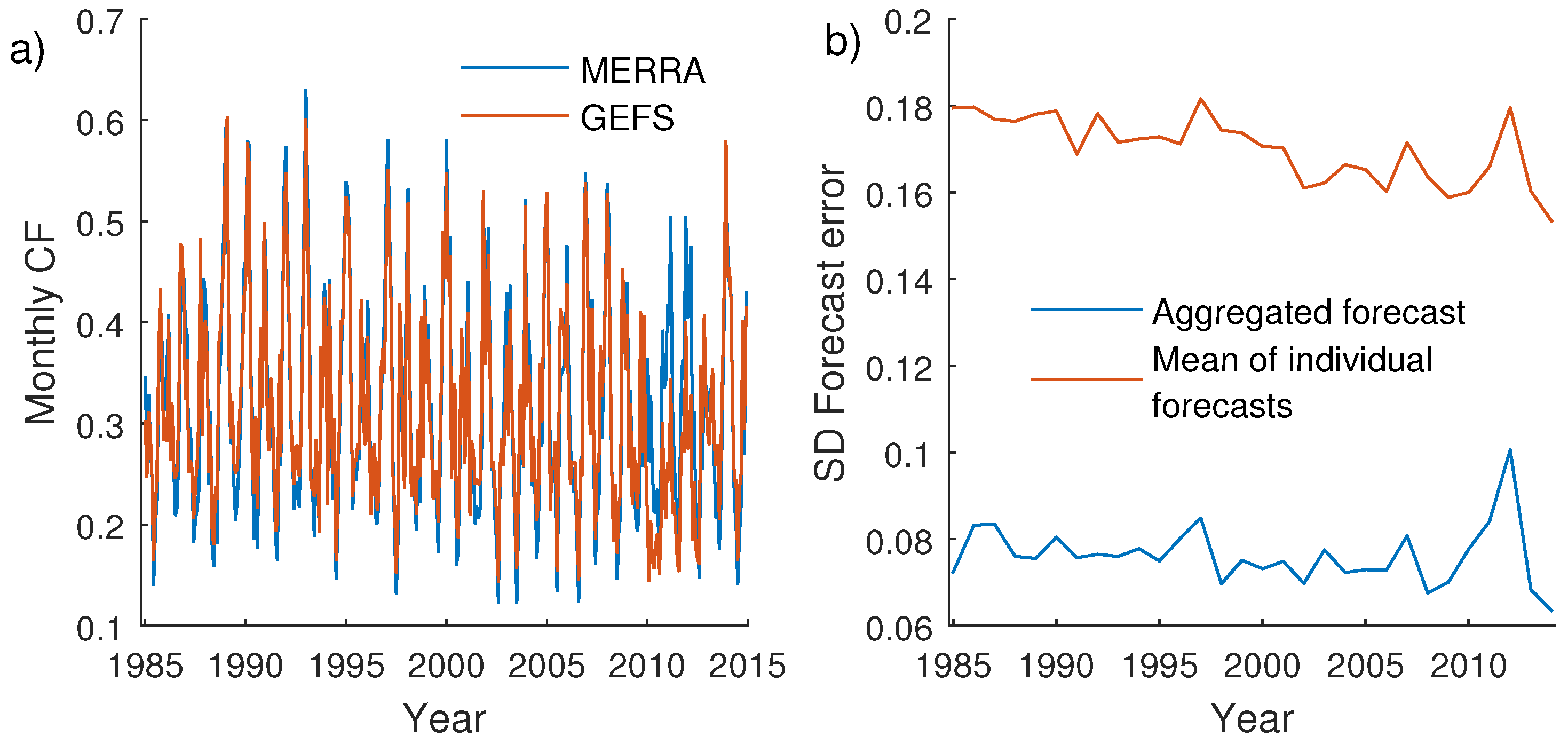
We begin by evaluating how the SDs of day-ahead FEs from the raw GEFS model have evolved over time. Fifty farms in Sweden were randomly drawn. A mean wind speed of 6.8 m/s were assumed both for generation (MERRA) and forecasts (GEFS) for all sites. This may seem overly simplistic, but as shown in [48], good projects are available in almost the entire country and the distribution of farms is relatively even. Figure 3a shows the monthly CFs from both models. In general, these agree well except for year 2010–2012, which is likely due to a change in source for GEFS initial conditions. It also seems that GEFS slightly underestimates the monthly variability as compared to MERRA.

In Figure 3b, SDs of FEs are given for each year. The blue curve shows the annual SDs of aggregated FEs and the orange curve shows the mean annual SDs of FEs for individual farms. The SDs are relatively time invariant. Quoting [43] (page 2), “As discussed in the journal article [42] this data set is generally statistically consistent with the operational 00 UTC run of the GEFS. However, due to recent changes in the data assimilation procedure and the changes in the observing network over time, more recent forecasts are generally more accurate than older forecasts”.

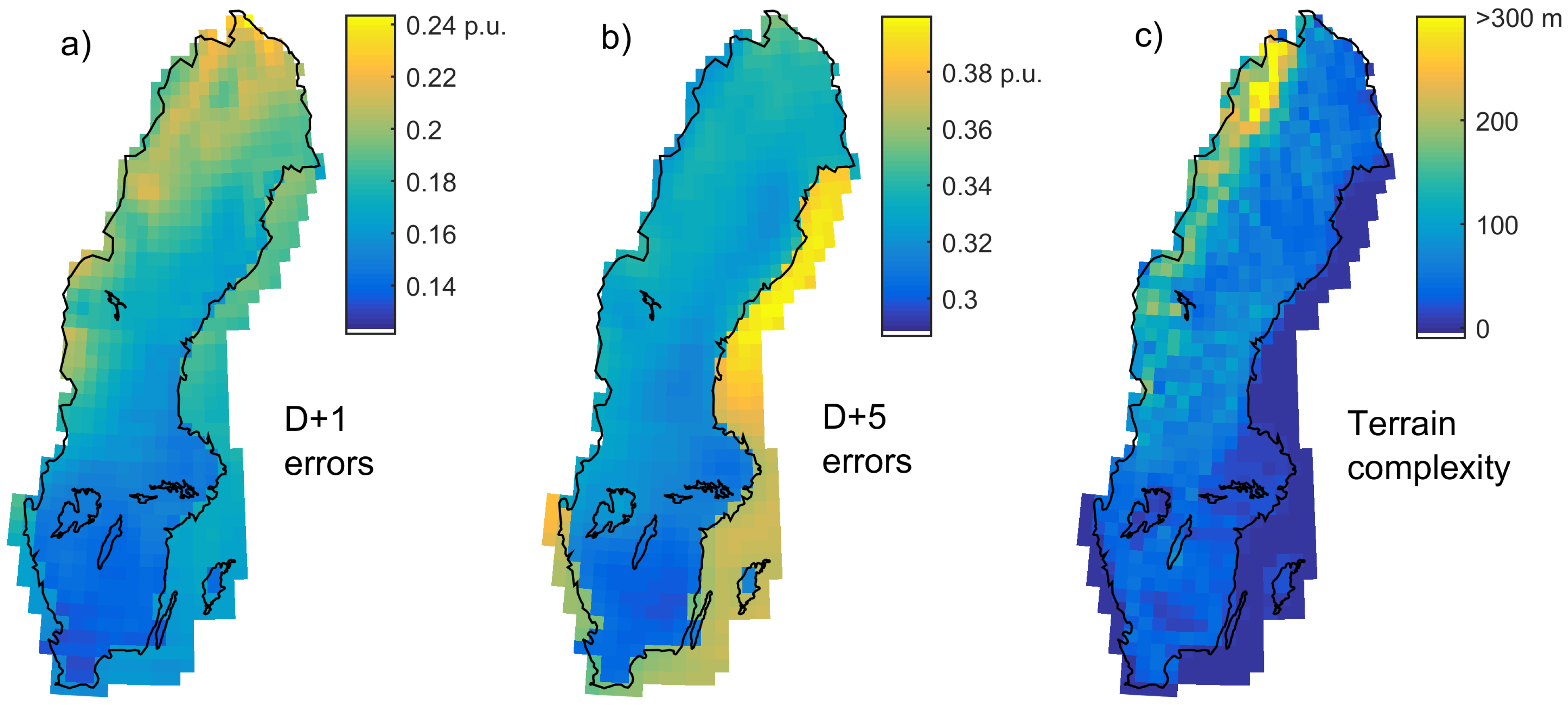
As shown in [28], the magnitude of FEs depends on the terrain complexity. We therefore performed a test on how the raw GEFS day-ahead FEs varied over Sweden. As for our previous example, a “correct” mean wind speed was assumed for GEFS but no other manipulation was performed. For onshore grid cells, a mean wind of 7 m/s and a specific rating (generator rating over rotor area) of 300 W/m² were assumed, resulting in a CF of around 0.34. For offshore grid cells, the corresponding figures were 8.5 m/s, 350 W/m² and 0.44. Ten- year-long time series were calculated for D + 1 and D + 5 forecasts. As can be seen in Figure 4, the D + 1 errors for onshore grid points are strongly related to the complexity of the terrain as quantified by the standard deviation of ground heights within each grid cell (Figure 4c). A lot of validation data would be necessary to determine if the relative differences are correct, but results from [28] at least suggest them to be reasonable. Note that when noise is added to GEFS (see Section 3.2), the differences are reduced. For D + 5, the errors are largest for offshore grid cells, at least when expressed in relation to the installed capacity as in the figure. The terrain-dependence for onshore errors is much weaker for this horizon.

4.1. Case Study—Belgium

Generation time series and up to week-ahead forecasts were modelled for all major farms in Belgium and the resulting aggregated FEs were compared to measurements from the Belgian TSO. The average CFs were estimated at 0.41 for offshore farms and 0.22 for onshore farms (with slight variations according to the specific ratings of the WTs). This gave a relatively good match of modelled and actual generation; correlation 0.97 and root-mean-square error 0.066 p.u.

For the added noise, it was found that an ARMA(2,2) model suited our needs. The fitted model was

$$Y_t=1.090Y_{t-1}-0.1930Y_{t-2}+{\epsilon }_t-0.1135{\epsilon }_{t-1}-0.2133{\epsilon }_{t-2},{\epsilon }_t\in \mathcal{N}(0,0.3358).$$

(3)

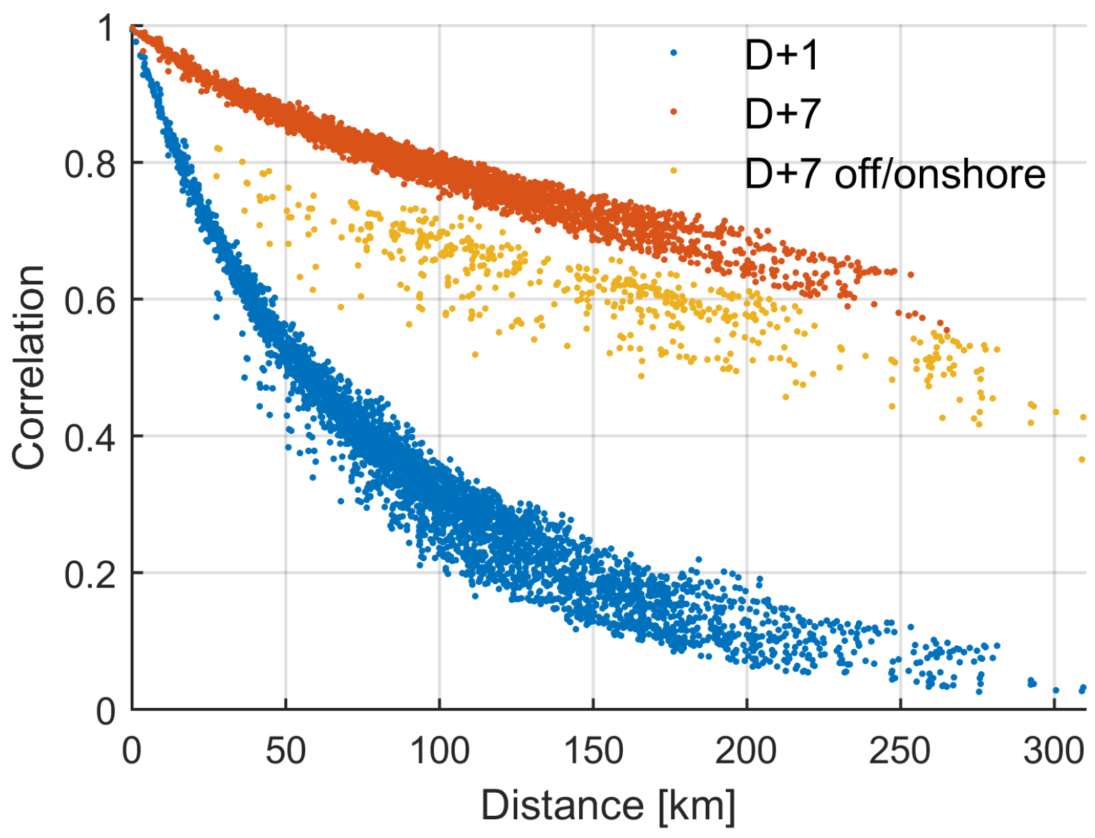
For the multivariate ${\epsilon }_t$ time series, a decay coefficient of $D=50$ km was found appropriate. In order to get correct error magnitudes for both D + 1 and D + 7, the noise time series were multiplied with 1.5, 90% of the bias was removed (${\mu }_{fix}=0.9$) and 28% of the wind speed error each hour was removed ($e_{fix}=0.28$).

Correlations of modelled FEs versus separation distance are given in Figure 5. The D + 7 correlations between onshore and offshore farm pairs (shown in yellow) are lower than for other D + 7 observation pairs, indicating different wind climates onshore and offshore.

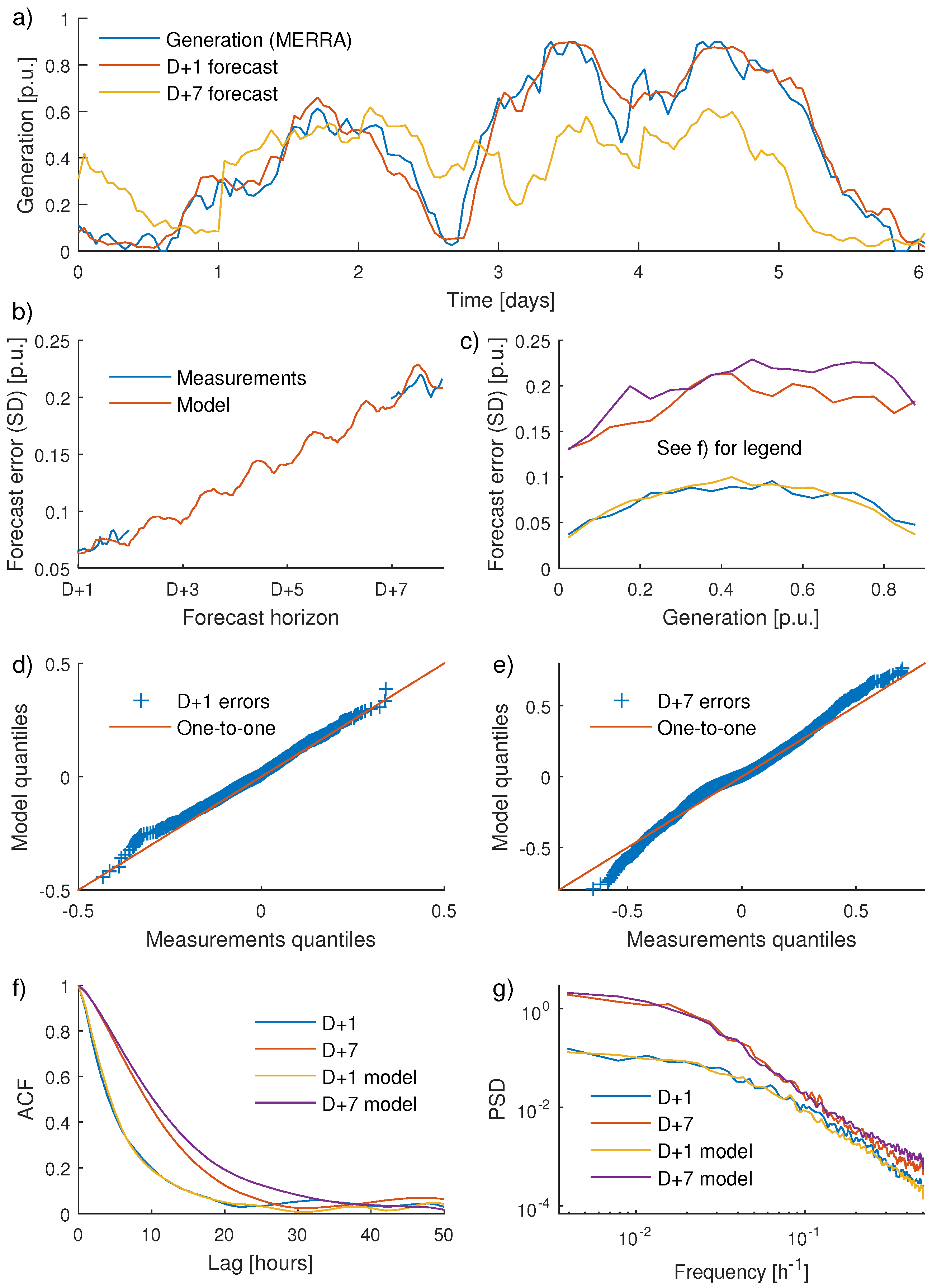
An example of modelled forecasts as well as a comparison between characteristics of measured and modelled FEs are given in Figure 6. An example of modelled generation and synthetic D + 1 and D + 7 forecasts is first presented in Figure 6a. Note that towards the end of day two, there is a phase error in the D + 1 forecast; the generation ramps up slightly earlier than the forecast. These types of errors, also present for operational forecasts, are generally not captured with purely statistical methods for generating synthetic forecasts. Also note the abrupt change in the D + 7 forecast at the beginning of day one. Similar step changes can be seen when actual forecasts are updated, especially for longer horizons.

Figure 6b shows how the FEs for operational and synthetic forecasts depend on horizon. The good agreement should not come as a surprise since the model parameters were tuned to give a good match. In Figure 6c, the impact from generation level on FE magnitude is displayed. For D + 1, model and measurements both give highest errors when the national generation is around 0.2–0.7 p.u. During these occasions, it is likely that many WTs are operating in the steepest part of the power curve. For D + 7, the curves are not agreeing as well, but both model and measurements give lower errors for very low national generation levels. Quantile-quantile plots for measured and modelled FEs are given in Figure 6d,e. The distributions agree well, also in the tails. This is beneficial since the extreme errors are important for dimensioning of the reserves. The D + 1 autocorrelations given in Figure 6f have an excellent match. For D + 7, the autocorrelation is, however, somewhat overestimated by the model. Figure 6f, finally, shows PSD estimates for model and measurements.

Matlab code and time series of measured and modelled generation and forecasts for Belgium can be sent upon reasonable request.

4.2. Case Study—Sweden

When generating forecasts for three farms in Sweden, the same ARMA model as for Belgium was used, including the multiplier of 1.5. Subsequently, 35% of the wind speed error for each hour was removed, i.e., slightly more than for Belgium. The latter seems reasonable since separate, trimmed operational models were used for the farms in Sweden, whereas in Belgium, the forecasts were made for the national aggregated generation. Note that the use of the same noise model for Belgium and Sweden was a deliberate choice; although somewhat better performance (i.e., similarity to measurements) could be obtained by using separate parameters, it is beneficial to show that one model works well for both countries and both for individual farms and for national output, thereby demonstrating the robustness of the method.

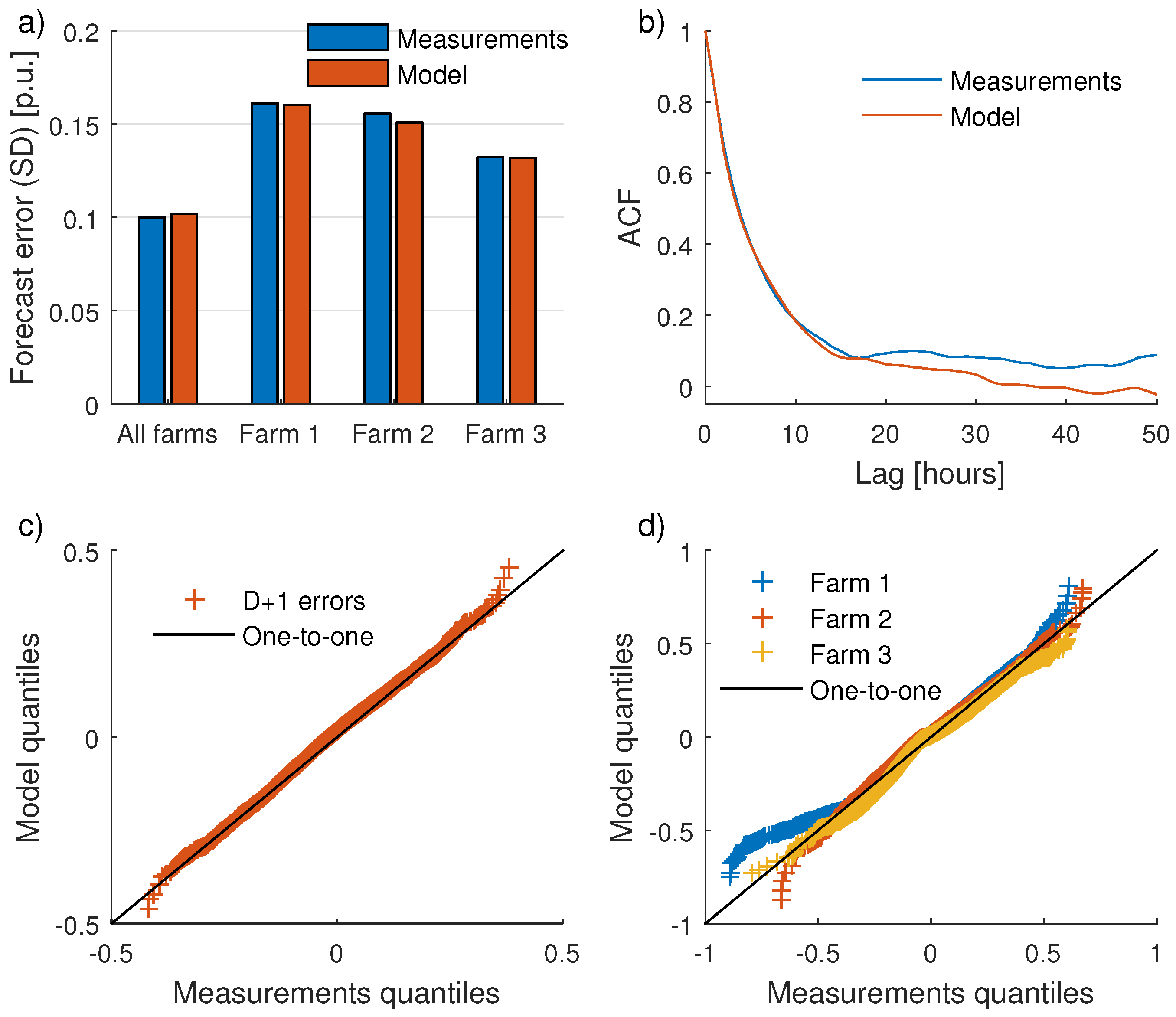
Validation results for day-ahead forecasts are given in Figure 7. First, in Figure 7a, it is demonstrated that when $e_{fix}$ is tuned to give a correct magnitude of the errors for all farms combined, the magnitude of the errors for individual farms are also appropriate. Since data were only available for three farms, it is hard to determine if the model is able to quantify the FE magnitude for farms in different terrain complexity and with different WT characteristics, but the results look undeniably promising. Farm 1 is located in complex terrain and has high errors. Farm 2 is an offshore farm with higher CF than the other two farms. Farm 3, which has lowest errors both for measurements and model, is an onshore farm in somewhat hilly terrain, bordering flat terrain near the sea in the prevailing wind direction. Figure 7b shows the autocorrelations for aggregated FEs. In Figure 7c,d, finally, Q–Q plots are given for aggregated and individual FEs respectively.

4.3. Influence from WT Characteristics

An important purpose of a model of wind power forecasts is the evaluation of the forecast errors for different scenarios of future wind farms. In a technical report [48], it was shown that the variability of wind power generation (in Sweden) can be reduced significantly by increasing the average capacity factor, which can be accomplished by, for example, increasing the share of offshore farms, increasing the hub heights or lowering the specific ratings. An interesting question is whether the reduced variability also leads to lower forecast errors. This is the topic for the current section.

Four different scenarios were considered: S1 with a CF around 0.30 and S2–S4 with CFs around 0.36. S1–S3 consist of 50 randomly selected onshore farms in Sweden. The same farms were used for all scenarios. In S4, fifteen of the farms were replaced with five offshore farms (within 50 km from the shore), each with three times higher installed capacity than an onshore farms. Some characteristics of the scenarios are given in

Table 2. Farm characteristics in the different scenarios. 30% of the installed capacity in S4 consists of offshore farms, all other scenarios have only onshore farms.

		Mean Wind	Specific Rating	Capacity Factor
S1	Onshore	7 m/s	350 W/m2	0.30
S2	Onshore	7 m/s	260 W/m2	0.36
S3	Onshore	7.6 m/s	350 W/m2	0.36
S4	Onshore	7 m/s	350 W/m2	0.36
	Offshore	9 m/s	350 W/m2

. As compared to the base scenario (S1), the higher capacity factors in S2–S4 were obtained by reducing the specific rating (S2), increasing the hub heights, and thereby the mean wind speeds (S3), and by assuming 30% of the installed capacity as offshore farms (S4). For the forecast modelling, the same assumptions as in Section 4.2 were used.

Since the results to some degree depend on the stochastic selection of farm locations, ten realisations were performed and averaged results are presented below. Standard deviations of day-ahead and week-ahead forecast errors for the four scenarios are given in

Table 3. Impact from wind turbine characteristics on forecast errors. Results for 50 hypothetical farms in Sweden for horizon D + 1 and D + 7. All results are given as standard deviations of forecast errors in p.u., normalised both to installed capacity (P) and annual energy yield (E).

	D + 1 (P)	D + 7 (P)	D + 1 (E)	D + 7 (E)
S1	0.0587	0.155	0.193	0.510
S2	0.0633	0.167	0.177	0.465
S3	0.0637	0.167	0.177	0.466
S4	0.0564	0.160	0.158	0.448

. The results are given both normalised to the installed capacity (as earlier in the paper) and normalised to the annual energy production. The latter can be more relevant when comparing different paths of future wind power deployment; it is, in our opinion, generally more interesting to study the variability, forecastability, etc. for a certain amount of produced energy than for a certain installed capacity.

As can be seen in Table 3, it is clearly beneficial with more offshore wind (scenario S4). For D + 1, the SD of FEs was reduced with 4% relative installed capacity and 18% relative produced energy as compared to S1. Note that a large part of the reduction is due to lower correlations between the FEs; the individual errors for offshore farms (relative installed capacity) were actually somewhat higher than for onshore farms. For D + 7, the corresponding figures were an increase of 3% and a reduction of 12% respectively, i.e., the benefits of more offshore wind are not as obvious for this horizon. When increasing the CFs of onshore farms by reducing specific rating or by increasing mean wind speed (S2 and S3), the errors relative installed capacity were increased by around 8%, whereas the errors relative produced energy were decreased by 8%–9%. It can be noted that the forecast error magnitudes are strongly correlated to the variability of generation quantified by the SD of one hour step changes. The relative changes of the latter metric for S2–S4 as compared to S1 were +10%, +11% and −3% when normalising to installed capacity and −7%, −6% and −18% when normalising to produced energy, i.e., very similar to the changes in day-ahead forecast errors.

5. Discussion

In wind integration studies, one possibility is to use historical, actual forecasts. Dedicated forecast systems (based on high-resolved NWPs) or purely statistical methods can also be used for producing the required forecast datasets. How do these methods compare to the one proposed in this paper? Historical forecasts have two main drawbacks: the time series are often relatively short and are given for a particular set of wind farms. If future scenarios are to be studied, these datasets are therefore of limited value for direct use in wind integration studies. If computational and monetary costs are not an issue, a high-resolved NWP system, taking future wind power scenarios and long reanalysis time series as inputs, is probably superior to all other methods. Unfortunately, costs are often an issue and other strategies are thus necessary. The most relevant comparison is therefore between our method and purely statistical ditto, see e.g., [8,32,33,34]. Disadvantages with our approach are that relatively large datasets need to be downloaded, processed and stored, that the computational cost can be higher (although only minutes on a standard desktop computer), and, most importantly, that the update frequency and ensemble size are limited by the reforecast dataset (once per day and eleven members for GEFS). The main advantage is that our approach gives forecasts with a physical coupling to the weather. This results are that the errors differ depending on terrain complexity, that the FE correlations can be different for farm pairs with the same separation distance, that the FEs can depend on the weather conditions (e.g., atmospheric stability, wind speed and wind direction), and that phase errors will be present and that consecutive forecasts are properly related.

Since operational forecasting systems regularly use such techniques, one can argue that a more advanced statistical post-processing could give more realistic synthetic forecasts. The post-processing system can take numerous variables as inputs and correct for biases related to previous errors as well as wind direction and many other meteorological variables. This can be particularly relevant if the errors are larger during some periods such as years 2010–2012 in Figure 3a. As an experiment, the impacts from using a Gradient Boosting (GB) [49] machine learning algorithm with Empirical Orthogonal Functions (EOF) of meteorological variables as predictors was evaluated. GB is an ensemble method based on classification and regression trees [50]. Although not one of the most common techniques for statistical post-processing of wind power forecasts, it has been previously used with some success [51]. See also [45,52] for examples of the use of GB and EOFs in the wind power field, including more detailed descriptions and references for further reading. By using the advanced post-processing, the SDs of FEs were reduced by 12%–14% and 10%–11% for D + 1 and D + 7, respectively. In principle, all seasonal bias and much of the bias for year 2010–2012 were removed.

Operational NWP models and post-processing techniques have improved over the last decades, leading to reduced forecast errors and it is likely that this trend will continue. When our model is used for generation of synthetic forecasts for future scenarios of wind farms, an important decision is how the anticipated improvement should be accounted for in the model. As shown in the previous paragraph, a post-processing module gives some FE reduction. If a further improvement is deemed likely, this is most easily implemented by increasing the $e_{fix}$ parameter. A higher $e_{fix}$ leads to a relatively uniform reduction of the errors, i.e., the extremes are reduced to the same extent as the SD. It is also reasonable to believe that the correlations between the forecast errors will be lowered. This can be implemented by reducing the decay parameter for generation of multivariate noise. The question is whether very large phase errors will exist also in a future when the SD has been cut to e.g., 50% of what it is today. On the contrary, will focus be on improving forecasts so that extreme errors are reduced more than the SD? Day-ahead FEs for the 50 Hertz system in Germany from 2009 to 2013 revealed that the SD was reduced from 6.4% to 4.4%. During this period, the excess kurtosis was stable around four and the 1st and 99th percentiles were also fairly stable in relative terms, with magnitudes of about three times the SD. In other words, extreme FEs were reduced at the same pace as the SD. For the German part of the TenneT area for years 2009–2013, the SD of D + 1 errors were around 6%–7% for the first three years and 3.7% and 4.7% for the last two years. Although the extremes relative to the SDs were not as stable as for 50 Hertz, it was hard to spot any clear trend.

If probabilistic forecasts are desired, this can be implemented in a straightforward fashion. With GEFS data, these will, however, be limited to one control member and ten perturbed members. In the present work, focus was on relatively long forecasts since our intention is to use the model for creating synthetic forecasts for simulating hydro power planning in a future with a significant penetration of wind power. Thus, it was not deemed a problem that GEFS reforecasts are only issued once per day. For shorter planning (intra-day or day-ahead), it can however be desirable with forecasts updated several times daily. Forecasts from the TIGGE project might be a better option for these applications.

6. Conclusions

In the present work, a new method for generating synthetic wind power forecasts for power system studies is presented and the model output is validated with actual forecasts. The main idea is to use coarse reanalysis data (MERRA in our case) for modelling wind power generation and GEFS reforecasts with some statistical processing to produce synthetic forecasts. This enables us to generate 30+ year time series of relatively consistent quality.

Earlier methodologies for synthetic forecast generation can broadly be classified as based on operational forecasting systems fed with high-resolved data or as purely statistical methods. The former approach is the most realistic, but due to the very high computational and monetary costs, it is rarely used in practice. Statistical methods are much faster, but are not able to truly capture all relevant aspects of real forecasts and forecast errors. In this paper, we show that our method is able to provide realistic forecasts at a reasonable computational cost. Furthermore, the required input data is freely and globally available.

Examples of characteristics of actual forecast (errors) that can be faithfully represented by the model include: distribution, autocorrelation and power spectral density of FEs for different horizons, abrupt changes when forecasts are updated, correlation of FEs and the existence of level and phase errors. The influence from terrain complexity on modelled FE magnitude is promising, but more data is necessary for a proper validation. The same holds for variations of FE correlations, e.g., that errors for an onshore and an offshore farm are less correlated than for two onshore farms with the same separation distance.

As an application of the model, FEs were studied for different scenarios of future wind farm characteristics. It is shown that an increased capacity factor of onshore farms give higher errors relative to the installed capacity but lower errors relative to the produced electricity. By assuming 30% capacity from offshore farms, the aggregated errors normalised to energy production were lowered considerably.