Data-Driven Baseline Estimation of Residential Buildings for Demand Response ^†

Abstract

The advent of advanced metering infrastructure (AMI) generates a large volume of data related with energy service. This paper exploits data mining approach for customer baseline load (CBL) estimation in demand response (DR) management. CBL plays a significant role in measurement and verification process, which quantifies the amount of demand reduction and authenticates the performance. The proposed data-driven baseline modeling is based on the unsupervised learning technique. Specifically we leverage both the self organizing map (SOM) and K-means clustering for accurate estimation. This two-level approach efficiently reduces the large data set into representative weight vectors in SOM, and then these weight vectors are clustered by K-means clustering to find the load pattern that would be similar to the potential load pattern of the DR event day. To verify the proposed method, we conduct nationwide scale experiments where three major cities’ residential consumption is monitored by smart meters. Our evaluation compares the proposed solution with the various types of day matching techniques, showing that our approach outperforms the existing methods by up to a 68.5% lower error rate.

1. Introduction

Evolving information and communications technologies in the energy industry, including smart meters and smart grids enable companies to forecast demand, characterize customer usage patterns, and utilize renewable energy more efficiently. Simultaneously, such advances also generate unprecedented volume of data that could bring huge impact on energy usage. Hence, data management and advanced analytics are required to transform data into recognizable insight on customer side. Specifically, demand side management programs that attempt to influence customer’s behavior require the combination of data about customers, consumption, and weather information to develop effective programs. They mainly consist of two major components: demand response (DR) and energy efficiency [1]. DR is often referred to as a virtual power plant since it allows utilities to treat it as another operational power plant by reducing the electricity load [2].

DR program is classified into two categories whether it is dispatchable or non-dispatchable. A dispatchable program can be initiated by utility to decrease the electricity demand in a relatively short time frame. In a dispatchable program, DR has several sub-programs. For instance, economic DR is the program triggered by energy price and demand bidding. This resource can be traded in the electricity market where real and reactive power are also traded. Thus economic DR competes with the power generators in the market. Another program is capacity resource program or emergency DR triggered by grid operator. In this scenario, controllable demand can be switched off by participants who receive incentives for shedding load, or directly controlled by grid operator. On the other hand, DR with non-dispatchable load falls into a category of time dependent pricing such as time-of-use (TOU), critical peak pricing (CPP), and real time pricing (RTP). TOU tariffs segment each billing month into hourly windows with different pricing levels; basic TOU scheme is to set different prices for on-peak and off-peak hours. CPP tariffs have a peak period in addition to TOU. Generally, the critical peak period could be executed on any given day with relatively high energy price. This induces customers to change their electricity consumption patterns to avoid critical peak price. RTP is a highly flexible pricing DR program without DR events. The price is determined by usage and this time varying price will affect customers to change their load patterns.

Recently, the independent system operators (ISOs) make efforts to implement DR programs to liberalize electricity markets and reduce extra generation cost. Since November 2014, buildings such as factories, large retail stores, commercial buildings in Korea are able to participate in economic DR program where DR resource is traded in the negawatt market operated by the Korea Power Exchange (KPX), the sole ISO in Korea. Note that this is just an initial step to build a deregulated energy market. As a result, negawatts produced by reducing electricity can be traded at the same market prices as real megawatts of generated electricity. For successful settle down of this new paradigm, DR program should precisely measure how much customers reduce their load during the DR event period, and thus measurement and verification (M&V) process is required to verify the amount of load reduction in this period. M&V is crucial because well-designed M&V can encourage a number of customers to actively participate in DR market. This process was developed to conduct the Implementation Proposal for The National Action Plan on Demand Response jointly issued by U.S. Department of Energy and the Federal Energy Regulatory Commission [3]. In this process, measurement quantifies this load reduction in kW or MW in 15, 30, 60 min for event duration, and verification provides evidence that the reduction is reliable.

Typical dispatchable DR programs give incentives to DR customers based on the amount by which they reduce their energy/power consumption. To verify the amount, customer baseline load (CBL) needs to be determined. CBL refers to the amount of electricity that would have been consumed by the customer if the DR event had not been occurred. The difference between actual load and CBL is considered as the amount of load reduction, i.e., the DR performance that the customer achieves. Hence, the accurate estimation of CBL is critical to the success of DR programs because it benefits all stakeholders by aligning the incentives, actions and interests of DR participants, utilities, and grid operators. Note that CBL play a key role in implementing DR programs; if the baseline is determined relatively low, customers are less motivated to participate in the DR program because they might think their performance is not fully acknowledged. On the other hand, if the baseline is estimated relatively high, utility companies are less motivated to operate DR program because the amount of load reduction is overly estimated and thus more incentive should be paid to customers [4,5] .

In the industry, two methodologies, day matching methods and regression analysis are the typical ways of constructing baseline load [6]. The day matching methods take a short historical period and calculate CBL by simply averaging the data of the previous non-event days. According to the report [7], for example, California ISO recommends customers to measure their performance by following North American Energy Standards Board M&V standard called Baseline Type 1. This is a simple average of 10 similar non-event days using most recent days prior to the DR event. PJM Interconnection, an ISO in the eastern United States, takes a high 4 days out of 5 days for the baseline. In the case of South Korea, KPX takes 6 days out of 10 days after removing two highest and two lowest days [8]. On the other hand, regression analysis is applied to build load prediction model for policymakers [9].

Besides baseline load estimation, load forecasting has been one of the most important research topics, and it is partially related with baseline estimation in terms of foreseeing certain period. Depending on the prediction range, there are two types of load forecasting: long-term load forecasting (LTLF) and short-term load forecasting (STLF). In some sense, STLF is similar to construct baseline load estimation since it investigates less than 24 h scale for load forecasting. Traditional statistical approach, namely, time series modeling is also developed to predict daily peak load and the load curve in [10,11,12]. Another widely adopted load forecasting method is based on data mining approach. The work of [13] reports that successful experiments are performed with artificial neural network (ANN) for solving STLF problem. Temperature and seasonal effects also have been considered for demand forecasting [14]. In [15], non-linearity between weather and consumption are investigated by means of a panel threshold regression model. In residential sector, such weather-related variables, building temperature, ambient temperature are used to build thermal load modeling to ensure the optimal operation in microgrids [16].

However, baseline estimation is not same as STLF since it must satisfy both consumers and utility side. The purpose of load forecasting for generation side is to match the amount of electricity generation to the consumption while minimizing generation cost. In contrast, the establishment of baseline load is aimed at demand side to measure the DR performance. The accurate demand forecasting can motivate customers to participate in DR programs and to receive monetary rewards from the utility company. The impact of choosing various baseline models with different implementation is evaluated based on real data in California, and the authors concluded that the acquisition of good weather data is a key to estimate the baseline [17]. Furthermore applying the morning adjustment factor can increase the accuracy of baseline models, and characterizing building loads by variability and weather sensitivity can determine types of baseline models [18].

Our main contributions in this paper are as follows. First, we apply new advances in data mining to develop CBL calculation with emphasis on customer consumption pattern in the morning. Two-stage adaptive architecture is proposed in this paper. Specifically, the Kohonen networks model is used to reduce the large data set into representative weight vectors. Then K-means clustering is applied to these vectors so that similar day patterns are grouped to build representative baselines. Second, typical residential buildings in Korea, known as high-story apartments, are used to demonstrate the proposed approach and to find out unique characteristics of residential consumption patterns compared to the case of non-residential buildings. Third, the evaluation of baseline estimation shows that our data mining technique outperforms the currently adopted methods. The numerical results indicate that our proposed algorithm has 20.9% to 68.5% less error rate compared to the day matching methods, specifically in summer season in terms of root mean square error and mean absolute error.

The rest of this paper is organized as follows. In Section 2, we set up the data mining structure for CBL calculation and propose our algorithm. Section 3 describes residential DR using real data gathered from various cities in Korea. Simulation results along with error sensitivity are illustrated and discussed in Section 4. Lastly we conclude our work with remarks in Section 5.

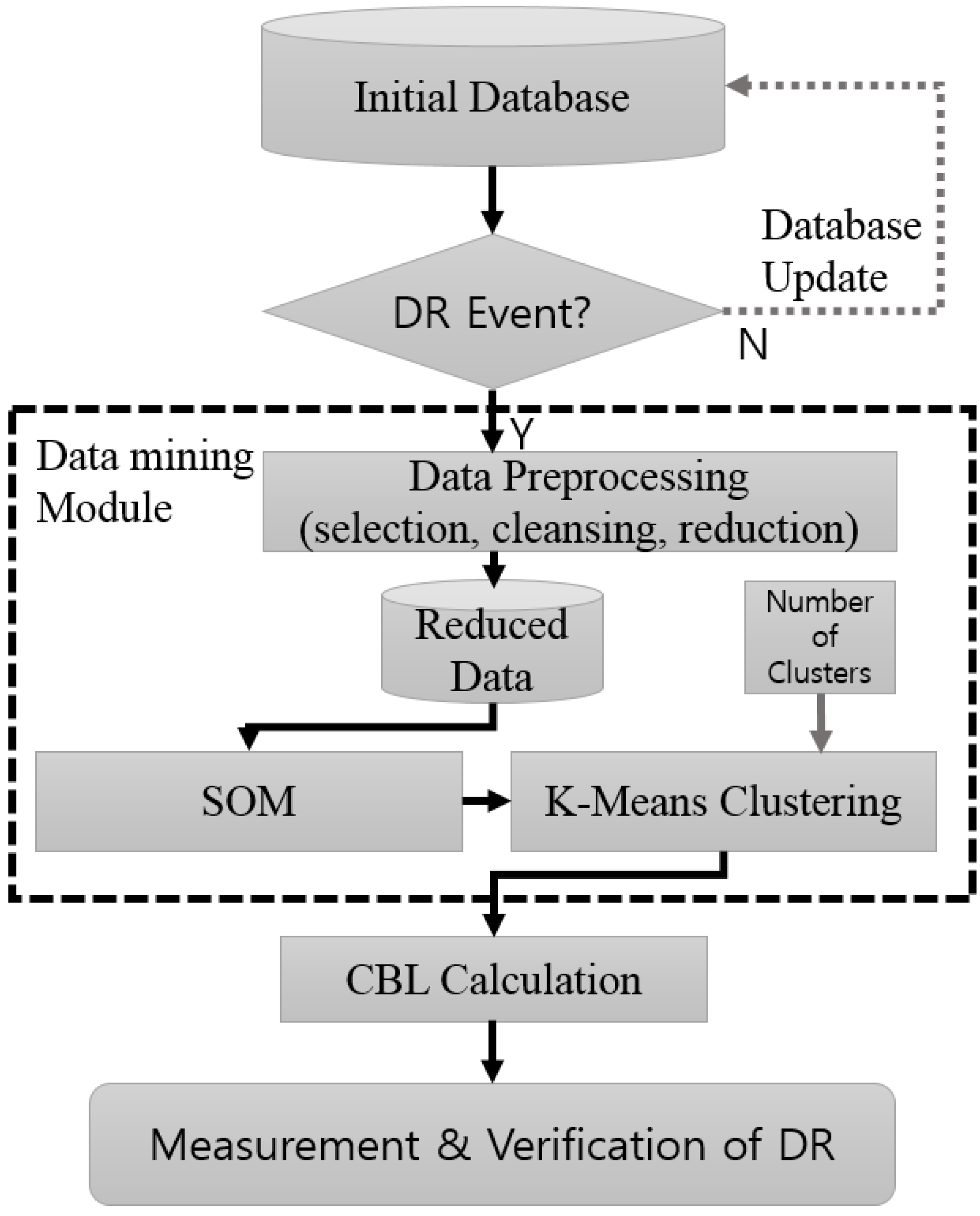
2. Data Mining Model

In this section, we describe a data mining framework to develop the CBL calculation as depicted in Figure 1. The framework of CBL is based on a knowledge-discovery in databases procedure supported by data mining techniques [19]. This procedure has been utilized to classify the electricity consumers in power system [20,21].

2.1. Data Preprocessing

The data mining model for CBL calculation is based on the unsupervised learning techniques. Before setting up a model for our work, data preprocessing is needed in advance. This is because some information could be distorted or missing during the period of collecting data or storing it to the utility server. This process includes three phases such as data selection, data cleansing and data reduction.

At first, in data selection, more relevant data is selected to process from the initial database. In our case, it is made according to the voltage level of the consumers. In data cleansing, we check the data inconsistency and find the outliers that distort the information about the customer facilities such as homes, factories or buildings. Inconsistent electricity consumptions are replaced by the average of daily consumption. In addition, some missing values are also replaced by daily average or removed according to the volume of missing data. Lastly, in data reduction, we reduce the data according to the load condition in terms of the seasons of year, and the type of weekday. This is because it is widely accepted that electricity consumption depends on the seasonal weather as well as the day type, i.e., either week or weekend [22].

Figure 1. Framework for the baseline load computation. DR: demand response; SOM: self organizing map; CBL: customer baseline load.

Figure 1. Framework for the baseline load computation. DR: demand response; SOM: self organizing map; CBL: customer baseline load.

The electricity consumption pattern of each day is then characterized by a curve called load profile. The representative daily load profile of the day $i\in \{1,\cdots ,N\}$ is a vector ${\mathbf{l}}_i=\left\{l_i\left(h\right)\right\}$ where $l_i\left(h\right)$ is the normalized values of the instant power consumed in the period of $h\in \{1,\cdots ,H\}$ where H is the total number of periods in a day, e.g., $H=24$.

2.2. Self-Organizing Map (SOM)

SOM is a feedforward neural network that uses the unsupervised learning introduced by Kohonen [23]. SOM belongs to a general class of artificial neural network methods, which are non-linear regression techniques to organize data so that unknown patterns are disclosed. SOM operation transforms a multi-dimensional input space onto a topology-preserving output space with greatly reduced dimension where neighboring neurons (or units (We use the neuron and the unit interchangeably)) respond to similar input vectors. The output space is called the grid of map units and denoted by $\mathcal{S}$. Each unit $\mathbf{s}\in \mathcal{S}$ is represented by a weight vector $\mathbf{s}=(s_1,\cdots ,s_D)$ where D is the dimension of the input vector. Each unit is logically connected to its adjacent units by the neighboring relationship. SOM is trained iteratively. Initially, all weight vectors have uniformly random values on [0,1]. Then, at each training step, the input vector denoted by $\mathbf{x}$ is randomly selected from the input data set, and the distance between $\mathbf{x}$ and all map units are computed. The best matching unit, denoted by $\mathbf{b}\left(\mathbf{x}\right)$, is the closest to $\mathbf{x}$, i.e.,:

$$\mathbf{b}\left(\mathbf{x}\right)=\underset{\mathbf{s}\in \mathcal{S}}{argmin}\parallel \mathbf{x}-\mathbf{s}\parallel$$

(1)

where $\parallel ·\parallel$ is the Euclidean norm. Then, the map units are updated as follows. The best matching unit of Equation (1) and its close neighbors are moved such as:

$$\mathbf{s}(t+1)=\mathbf{s}\left(t\right)+\alpha \left(t\right)h_{bs}\left(t\right)(\mathbf{x}-\mathbf{s}\left(t\right))$$

(2)

where t is the iteration index, $\alpha \left(t\right)$ is the learning parameter and $h_{bs}\left(t\right)$ is the neighborhood relation function between $\mathbf{b}$ and $\mathbf{s}$ [23]; with increasing the distance between $\mathbf{b}$ and $\mathbf{s}$, $h_{bs}\left(t\right)$ goes to 0. The magnitude of the adaptation is controlled via the learning parameter $\alpha \left(t\right)$ that decays in iterations. This process is repeated for all input vectors so that map units effectively represent various patterns of daily load consumption. The operation of SOM with the input vectors and the structure of map units that is associated with U-matrix will be explain in detail with data in Section 3.

2.3. K-Means Clustering

Clustering refers to partitioning a data set into a set of disjoint clusters. The goal of clustering is to group the input vectors that are close to each other. This process is done without any prior knowledge about the data structure such as the number of groups, labels, sample members, etc. A widely adopted definition of clustering is to form a partition that minimizes the distances within the intra-clusters and maximizes the distances between the inter-clusters [24]. One type of non-hierarchical clustering is K-means clustering which partitions a data set into K clusters. In our case, given a set of outcome $\mathcal{S}$ of SOM operation and an integer K, the K-means algorithm searches for a partition of $\mathcal{S}$ into K clusters that minimizes the with-in groups sum of squared errors (WGSS). Mathematically it is given by [25] such as:

$$\begin{array}{c}\hfill \mathrm{minimize}P(\mathbb{W},\mathcal{Q})=\sum _{k=1}^K\sum _{j=1}^S{w}_{j,k}{d}^2({\mathbf{s}}_j,{\mathbf{q}}_k)\end{array}$$

(3)

$$\begin{array}{c}\hfill \mathrm{subject}\mathrm{to}\sum _{k=1}^K{w}_{j,k}=1,\forall j\in \{1,\dots ,S\}\end{array}$$

$$\begin{array}{c}\hfill w_{j,k}\in \{0,1\},\forall j\in \{1,\dots ,S\}\end{array}$$

$$\begin{array}{c}\hfill \forall k\in \{1,\dots ,K\}\end{array}$$

where $\mathbb{W}=\left\{w_{j,k}\right\}$ is an $S\times K$ partition matrix, $\mathcal{Q}=\{{\mathbf{q}}_1,{\mathbf{q}}_2,\dots ,{\mathbf{q}}_K\}$ is a set of centroid of each cluster ${\mathcal{C}}_k$ in the same domain, and $d^2(·,·)$ is the square of the Euclidean distance between two vectors. Note that K-means clustering is an NP hard problem, and Lloyd algorithm can be used to obtain a solution in an iterative way; the algorithm guarantees the convergence, but not necessarily to the optimum [26].

2.4. Proposed Algorithm for Baseline Load Estimation

Algorithm 1 Baseline Load Estimation Algorithm

1: procedure LoadProfile 2:     for $\forall l_i,i\in \{1,\cdots ,N\}$ do 3:         $x_1,\cdots ,x_{12}\leftarrow 12-\mathrm{h}\mathrm{load}\mathrm{of}{l}_i\mathrm{before}\mathrm{DR}\mathrm{event}\mathrm{time}$ 4:         $x_{13}\leftarrow \mathrm{average}\mathrm{temperature}$ 5:         $x_{14}\leftarrow \mathrm{morning}\mathrm{factor}$ 6:         $x_{15}\leftarrow \mathrm{working}\mathrm{day}\mathrm{indicator}$ 7:     end for 8:     repeat 9:         find the best matching unit of input vector as in Equation (1) 10:         update the map units as in Equation (2) 11:     until 12:     maximum number of iterations 13:     repeat 14:         assign map units to cluster and solve problem as in Equation (3) 15:         update cluster centers 16:     until 17:     no cluster changes 18:  end procedure

Table 1. Input vector for SOM operation.

Vector	Description
$x_1...x_{12}$	12 h consumption before DR activation
$x_{13}$	Average temperature
$x_{14}$	Gradient of the load consumption (optional)
$x_{15}$	Working day indicator (optional)

Table 1. Input vector for SOM operation.

Vector	Description
$x_1...x_{12}$	12 h consumption before DR activation
$x_{13}$	Average temperature
$x_{14}$	Gradient of the load consumption (optional)
$x_{15}$	Working day indicator (optional)

In this subsection, we propose an algorithm for calculating CBL. Basically this algorithm finds the most similar load patterns from historical data by applying two-stage approach: SOM and K-means clustering. This two-stage procedure, firstly using SOM to generate the reduced data set, and secondly, clustering them shows high performance compared with direct clustering in terms of relative conditional entropy [27]. The authors in [27] concluded that the knowledge of SOM has significantly reduced the uncertainty when it comes to compute the relative conditional entropy of clustering. Another benefit of this approach is the reduced computational cost. SOM efficiently transforms the high dimensional data space into two dimensional space. This also assists to handle noisy and outliers, which are critical problem when K-means clustering is directly applied. By combining these two models, we can create an accurate solution dealing with large data sets.

We develop a framework that calculates the baseline load using the measured data, which is summarized in Algorithm 1. Utilities may provide notification to customer when they expect DR event likely to occur. In this process, 12 h load profiles of customers prior to the DR event time and the past profiles are extracted from the database. Note that to improve the accuracy, we deliberately add two features, i.e., the average temperature and the specified morning factor into the input vector optionally. As shown in Table 1, $x_1$ to $x_{12}$ are the hourly consumption before DR event, $x_{13}$ indicates the average temperature in the morning (8:00 AM–12:00 AM). We set the morning factor $x_{14}$ as the gradient of the electricity consumption curves because the gradient contains useful information of finding the similar data. $x_{15}$ is a working day indicator.

Next step, the grid of map units is initialized randomly. Through the iterations of finding the best matching units and updating the units as in Equation (1) and Equation (2), respectively, the output of SOM operation is represented by units’ weight vectors. After SOM operation, all the input vectors are projected onto one of the map units. Then, K-means algorithm is used to group the weight vectors of the map units into K clusters. In the final step, we find the best similar patterns of electricity consumption in the past. By averaging hourly load from this outcome, the CBL is estimated.

Note that the proposed algorithm has two key differences with the existing CBL methods. First, unlike the day matching methods, we find the most similar day by matching pattern sequence in the morning. Second, we consider other parameters such as average temperature, the gradient of electricity consumption, and working day indicator. By learning process, SOM output describes the data structure by a matrix. Clustering output indicates the representative load of the database. Details are explained in Section 3.2.

3. Residential Demand Response (DR): Case Study

Non-residential sectors such as commercial and industrial buildings have been actively participating in DR, but residential DR is relatively untapped resource. According to the U.S. Energy Information Administration (EIA) outlook [28], the residential sector makes up 20 percent of total energy demand. With such a significant portion of energy usage, the importance of residential DR cannot be ignored even though each household consumption could be negligible. Therefore, aggregated residential load can play a pivotal role in DR market in the future. In [29], the evaluation of residential DR reports that customer-specific regression analysis is likely to well measure the DR performance. However there are still several issues such as validation of the accuracy of load estimates, modeling the effect of consecutively triggered events, modeling the effect of a day-ahead notice, estimating aggregate load impact under a voluntary tariff, etc.

Starting from 1997, the Omni system company, one of the leading advanced metering infrastructure (AMI) companies in Korea, initiated a smart grid project aimed at connecting residential units and apartment maintenance offices with their smart meters called automated telemetering system (AMSYS). Currently more than 90% of newly built apartments and houses in Korea adopted this system. We used 27 months of 60-min load data from January 2012 to March 2014. This data is obtained for research purpose under the agreement of residents with privacy protection.

In this section, real data for residential customers of three different cities, summarized in Figure 2a, are used to validate our data mining approach. Each apartment site is indexed as A, B, and C.

Figure 2. (a) Korean residential building information; (b) Apartment complex A (Seoul); (c) Apartment complex B (Daejeon); (d) Apartment complex C (Gwang-ju). Bright color indicates high energy usage.

Figure 2. (a) Korean residential building information; (b) Apartment complex A (Seoul); (c) Apartment complex B (Daejeon); (d) Apartment complex C (Gwang-ju). Bright color indicates high energy usage.

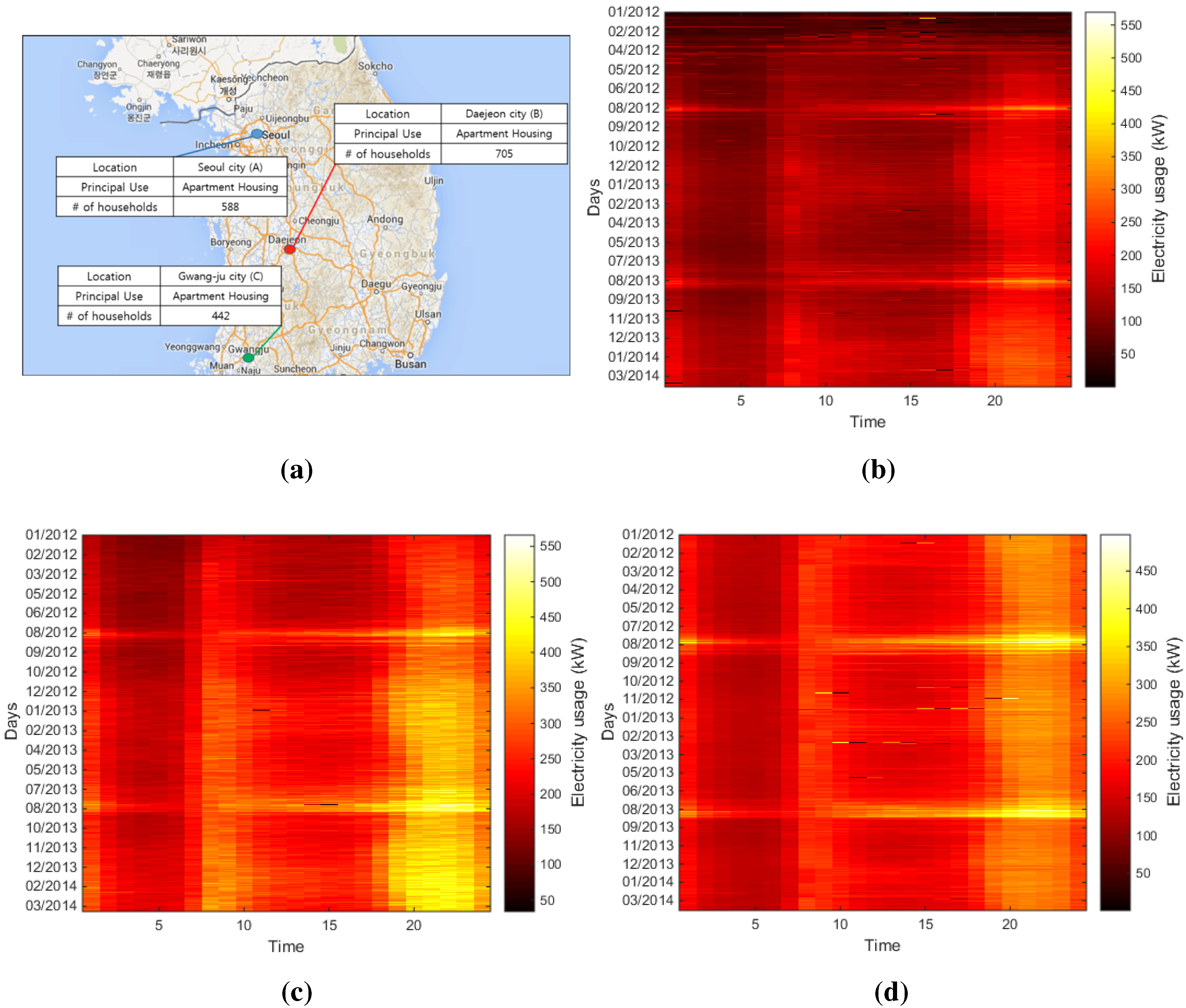
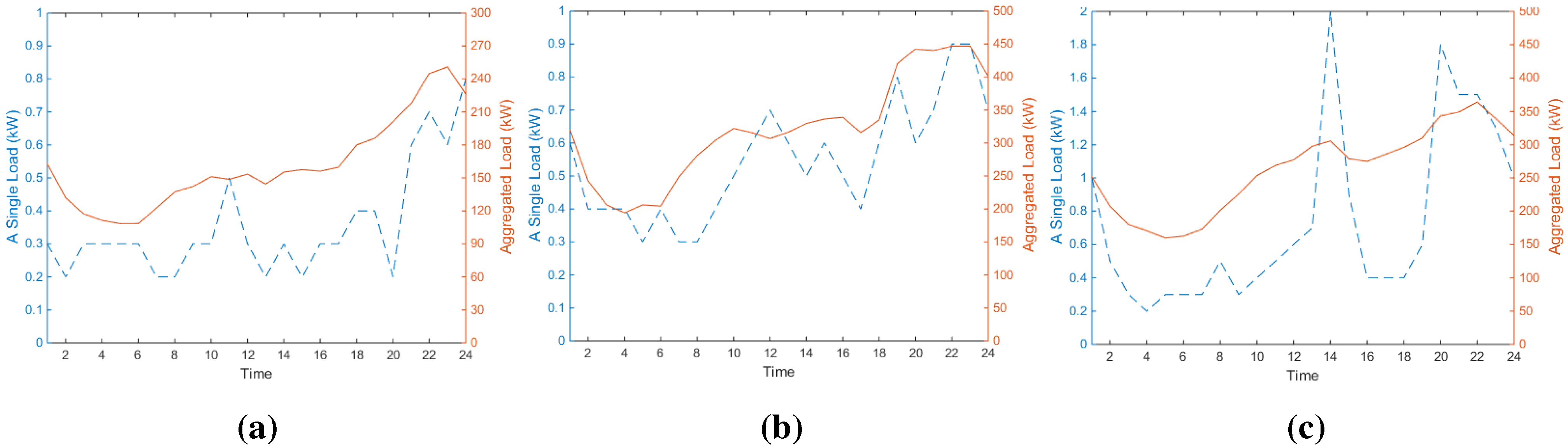
3.1. Load Characteristic

Figure 2 contains heat maps showing electricity consumption pattern for three testbeds from January 2012 to March 2014. As expected, it is observed in all cases that residential electricity consumption in summer (August 2012 and August 2013) is higher than that of other seasons in every time slot, which is due to thermostatic loads such as air conditioning. An interesting observation is that there are double peaks of load curve; in the morning, people wake up and start to use electricity, and in the evening, people come back home. This characteristic is clearly different from non-residential loads which typically reach a single peak in the afternoon [30].

Figure 3 shows a daily integrated load profile of all residential customers as well as a randomly selected single load profile from each residential site on 1 August 2013. It can be seen that household consumption across the day roughly follows the aggregated load profile; due to the nature of apartment residence, the type and size of household appliances may be similar to other neighbors. Comparing Figure 3a to Figure 3c shows that diverse morning temperature at that day (site A = $26.4{}^{\circ }\mathrm{C}$, site B = $29.4{}^{\circ }\mathrm{C}$, site C = $30.9{}^{\circ }\mathrm{C}$ in average) could affect consumption pattern of residents. It is clear that load consumption differs depending on both geographic location and the local weather.

Figure 3. Daily load profile for apartment residents across 24 h period on 1 August 2013: A sample of single residential customer load (dashed-lines) and aggregated load (solid-lines). (a) apartment complex A; (b) apartment complex B; and (c) apartment complex C.

Figure 3. Daily load profile for apartment residents across 24 h period on 1 August 2013: A sample of single residential customer load (dashed-lines) and aggregated load (solid-lines). (a) apartment complex A; (b) apartment complex B; and (c) apartment complex C.

3.2. Data Processing

As a few glitches can be seen in Figure 2, some of data in the database have bad quality. This corrupted data are corrected in the pre-processing phase; the outlier and outages are detected and replaced by regression techniques using the data of similar days. With this procedure, the quality of the data is enhanced with a minimal loss of information. These data are reduced and normalized using the procedure presented in Section 2. Other parameters such as temperature, the morning factor and working day indicator are considered as options into input vector.

In SOM operation, the number of neurons and size are determined by using heuristic approach. At first, the number of neurons is calculated by $5\sqrt{N}$ [31]. Recall that N is the total number of input data. Then, the shape of map units is formed by the ratio of the largest to second largest of eigenvalues. For example, in the case of site A, we use $9\times 11$ neuron architecture in SOM. Figure 4 is called the unified distance matrix (U-matrix) where each cell corresponds to a unit in S.

Figure 4. Unified distance matrix of input load profile.

Figure 4. Unified distance matrix of input load profile.

In U-matrix, the Euclidean distance between a unit and its six neighboring units is represented by the gray color of the unit. U-matrix gives insights about the local distance structure of the high dimensional data set and is widely used for the display of input data structure. For each unit in U-matrix, we assign the dark gray color to the unit that has a large number of close units. Similarly we assign the light gray color to the unit that has a small number of close units. The other shades of gray correspond to the level of distance between units. The circles inside the unit indicate how many input data points are projected on the particular unit. A larger circle means that many data points are assigned to the unit. U-matrix is able to keep the characteristics of the initial data with reduced dimensionality. These units are clustered in the second stage.

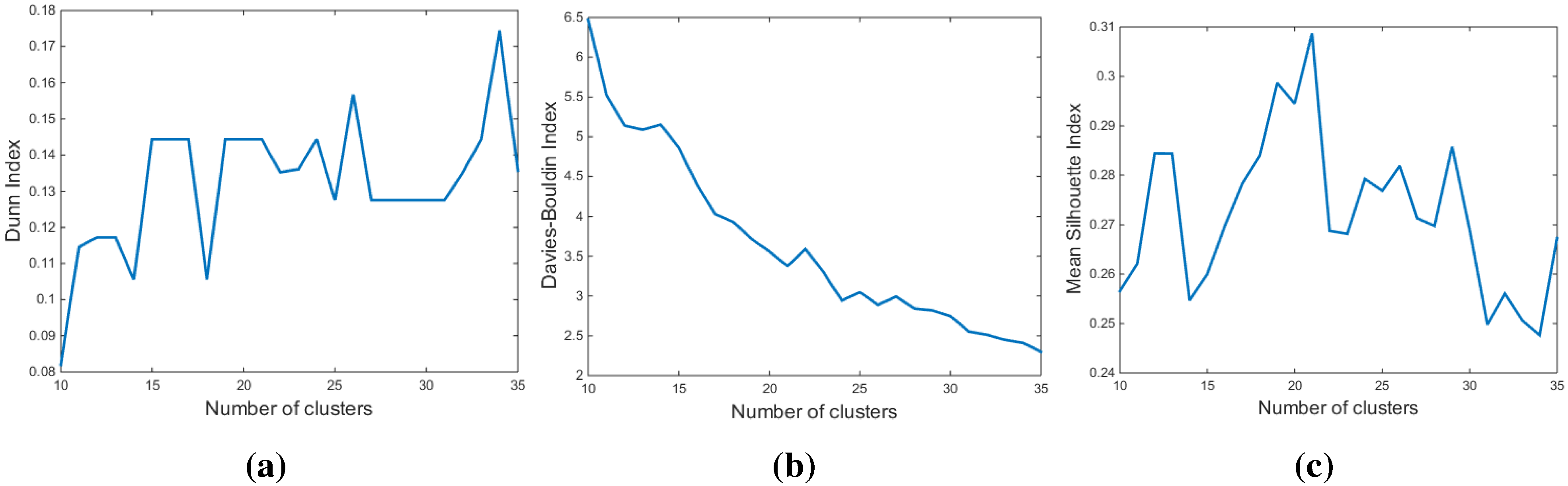
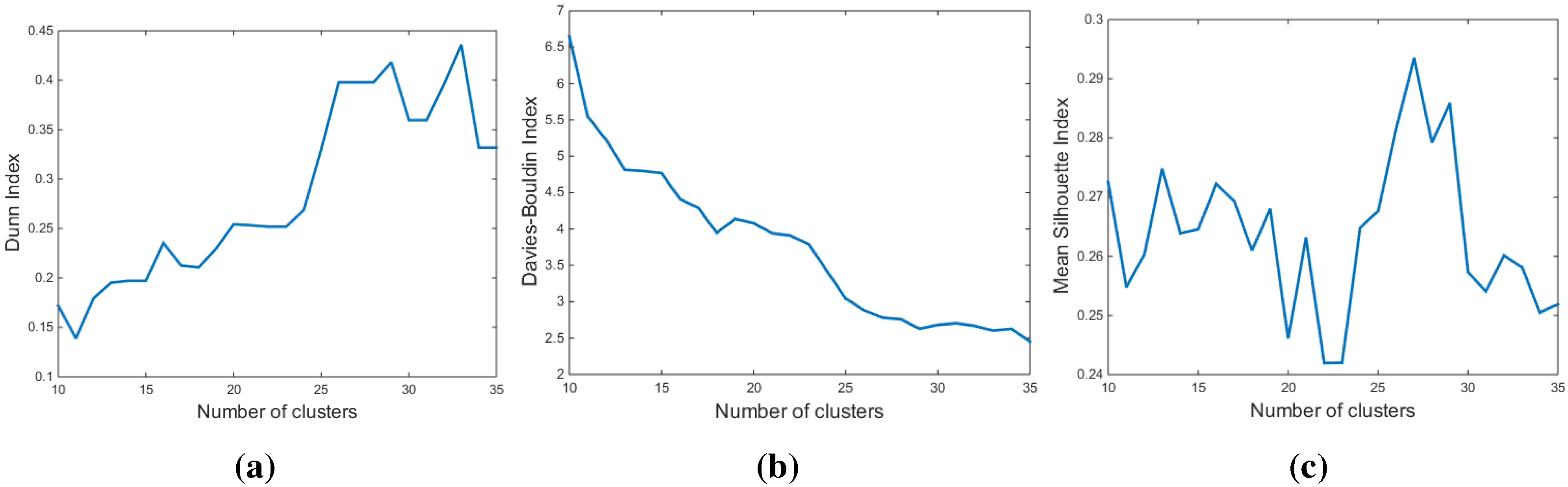
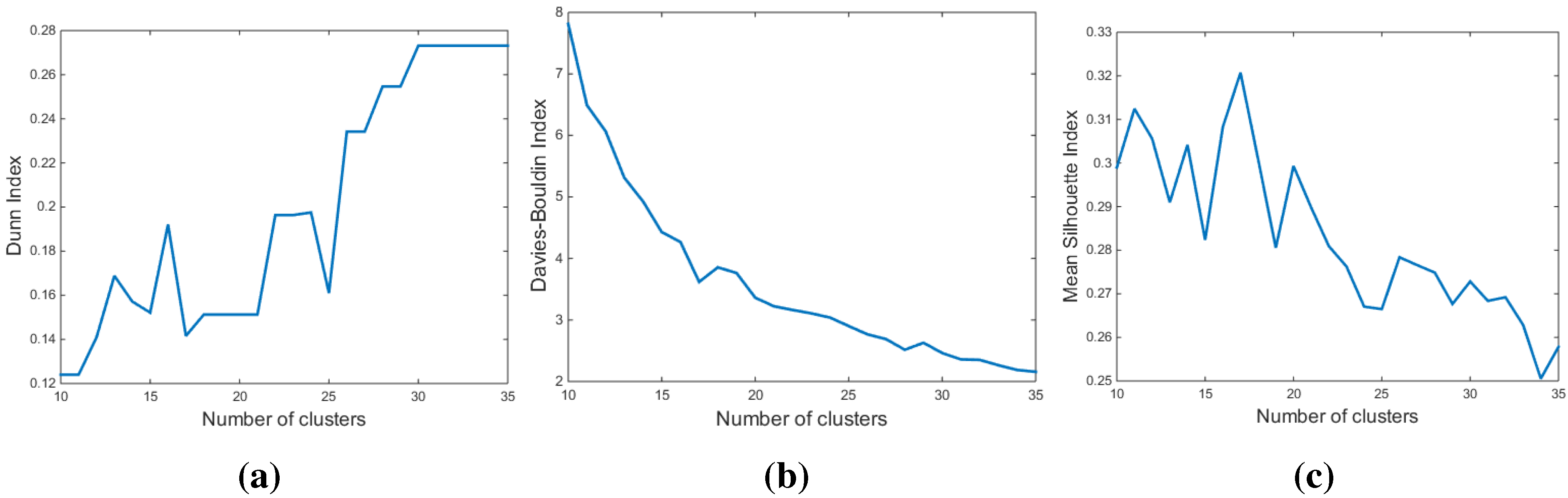
3.3. Determination of the Number of Clusters

In the unsupervised learning, the way of choosing a proper number of clusters has been discussed and emphasized in [21,32,33]. Recall that finding the number of cluster is an NP hard problem. Even though there are a large number of clustering validity indices, none of them guarantees the optimum number of clustering. We note that 24 dimensional time series data were clustered to forecast the behavior of energy time series in [33], which seems analogous to our approach. For this reason, we adopt three clustering validity indices as in [33]: the Dunn index (DI), Davies-Bouldin index (DBI), and mean silhouette index (MSI) to decide the number of clusters.

3.3.1. The Dunn Index (DI)

The DI is the ratio of inter-cluster to intra-cluster and widely used for finding the number of classes [34,35]. Obviously, a good clustering should have high dissimilarity between inter-cluster groups while minimizing that of intra-cluster members. The Dunn index with K number of clusters, denoted by $DI\left(K\right)$, is given by:

$$DI\left(K\right)=\frac{\min d({\mathcal{C}}_i,{\mathcal{C}}_j)}{\max \mathrm{diam}\left({\mathcal{C}}_m\right)}$$

(4)

where $d({\mathcal{C}}_i,{\mathcal{C}}_j)$ is the dissimilarity distance between clusters ${\mathcal{C}}_i$ and ${\mathcal{C}}_j$, and obtained by:

$$d({\mathcal{C}}_i,{\mathcal{C}}_j)=\underset{\mathbf{x}\in {\mathcal{C}}_i,\mathbf{y}\in {\mathcal{C}}_j}{\min }\parallel \mathbf{x}-\mathbf{y}\parallel$$

(5)

and $\mathrm{diam}\left({\mathcal{C}}_m\right)$ is the diameter of the m-th cluster and defined by:

$$\mathrm{diam}\left({\mathcal{C}}_m\right)=\underset{\mathbf{x},\mathbf{y}\in {\mathcal{C}}_m}{\max }\parallel \mathbf{x}-\mathbf{y}\parallel$$

(6)

High values of DI indicates that the data set is well separated and clustered.

3.3.2. The Davies-Bouldin Index (DBI)

The DBI identifies the validation of clustering algorithm by using quantities and features inherent to the data set [36]. Davies-Bouldin index for K clusters with ${\mathcal{C}}_i,i=1,\dots ,K$ is computed as follows:

$$DBI\left(K\right)=\frac{1}{K}\sum _{i=1}^K\underset{j\ne i}{\max }\frac{diam\left({\mathcal{C}}_i\right)+diam\left({\mathcal{C}}_j\right)}{d({\mathcal{C}}_i,{\mathcal{C}}_j)}$$

(7)

Note that, in this case, the average diameter of a cluster $diam(·)$ is given by:

$$diam\left({\mathcal{C}}_i\right)=\sqrt{\frac{1}{\mid C_i\mid }\sum _{\mathbf{x}\in {\mathcal{C}}_i}{\parallel \mathbf{x}-{\mathbf{q}}_i\parallel }^2}$$

(8)

where $\mid {\mathcal{C}}_i\mid$ is the number of members, and ${\mathbf{q}}_i$ is the centroid of cluster ${\mathcal{C}}_i$. Unlike DI, smaller value of DBI implies that K-means clustering algorithm separates the data set properly since each cluster is dense and isolated from other clusters.

3.3.3. The Silhouette Index (SI)

The SI is the method of measuring the separation among clusters suggested in [37] and defined as follows:

$$SI\left(\mathbf{x}\right)=\frac{c^{\prime }\left(\mathbf{x}\right)-c\left(\mathbf{x}\right)}{\max \{c\left(\mathbf{x}\right),c^{\prime }\left(\mathbf{x}\right)\}}$$

(9)

where $c\left(\mathbf{x}\right)$ is the average distance between $\mathbf{x}$ and all other vectors of the cluster $\mathcal{C}$ to which $\mathbf{x}$ belongs. $c^{\prime }\left(\mathbf{x}\right)$ is the minimum distance between vector $\mathbf{x}$ and other vectors in cluster $\forall {\mathcal{C}}^{\prime }\ne \mathcal{C}$ i.e.,:

$$c^{\prime }\left(\mathbf{x}\right)=\underset{\mathbf{y}\in {\mathcal{C}}^{\prime }}{\min }d(\mathbf{x},\mathbf{y})$$

(10)

The $SI\left(\mathbf{x}\right)$ ranges from $-1$ to $+1$ where large $SI\left(\mathbf{x}\right)$ represents adequate cluster and vice versa. Negative $SI\left(\mathbf{x}\right)$ means that $\mathbf{x}$ is mis-clustered. After that, mean silhouette index is obtained by averaging all the data points. So we can determine the number of classes in K-means clustering which has large silhouette index values.

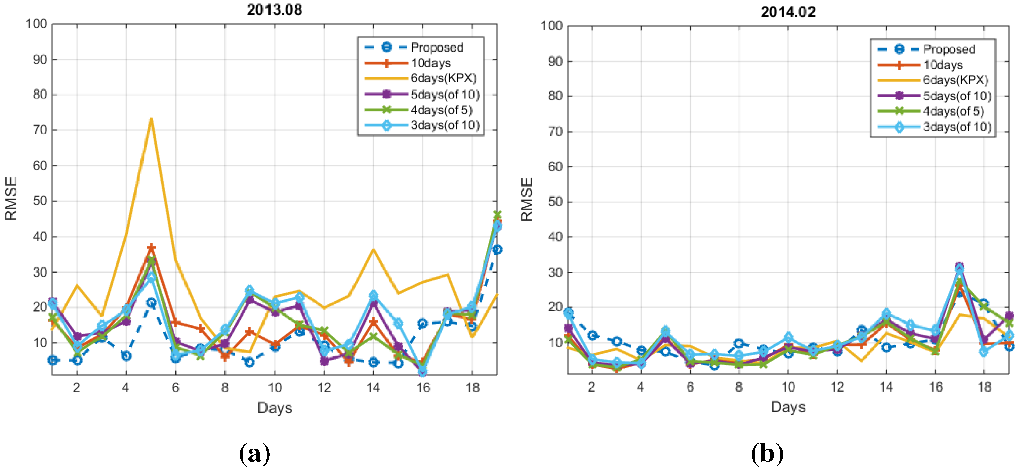
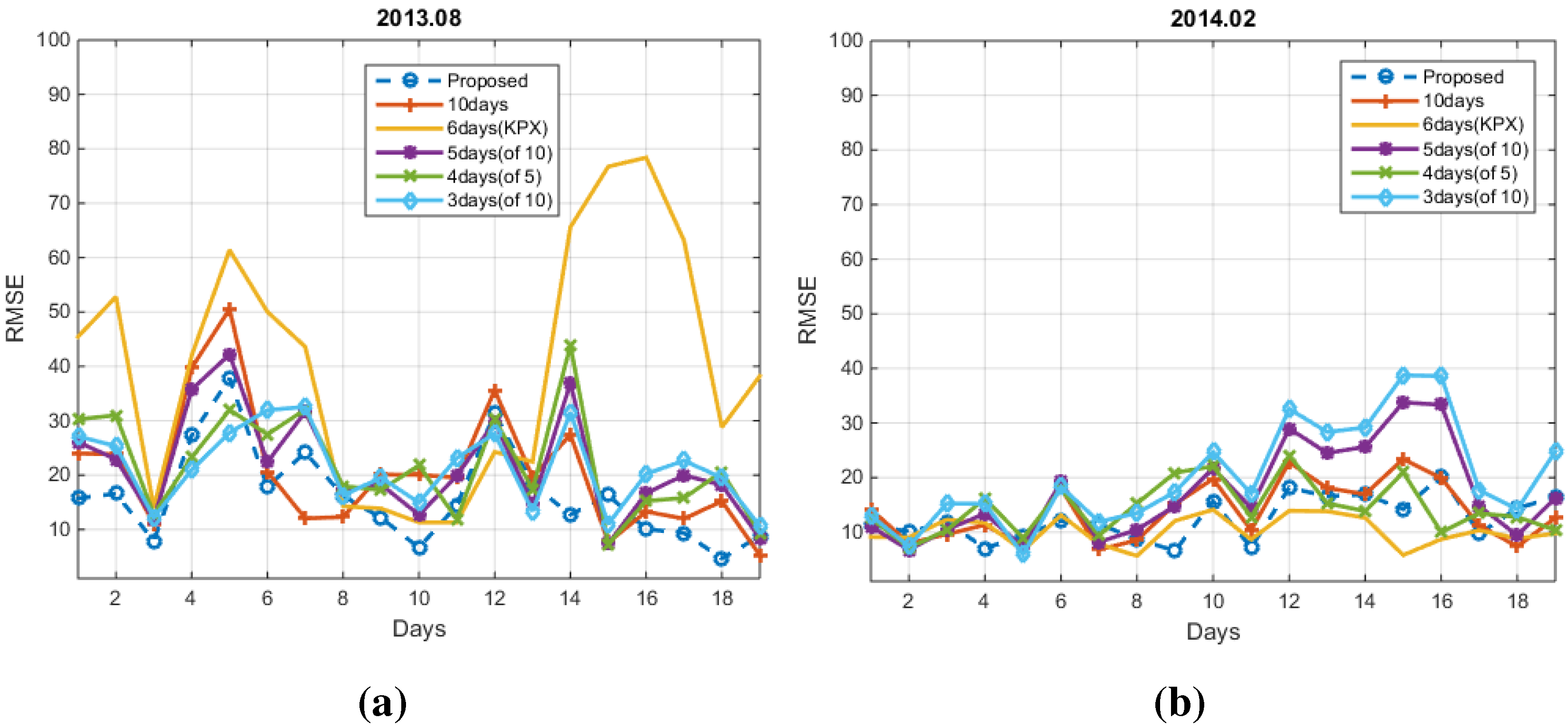
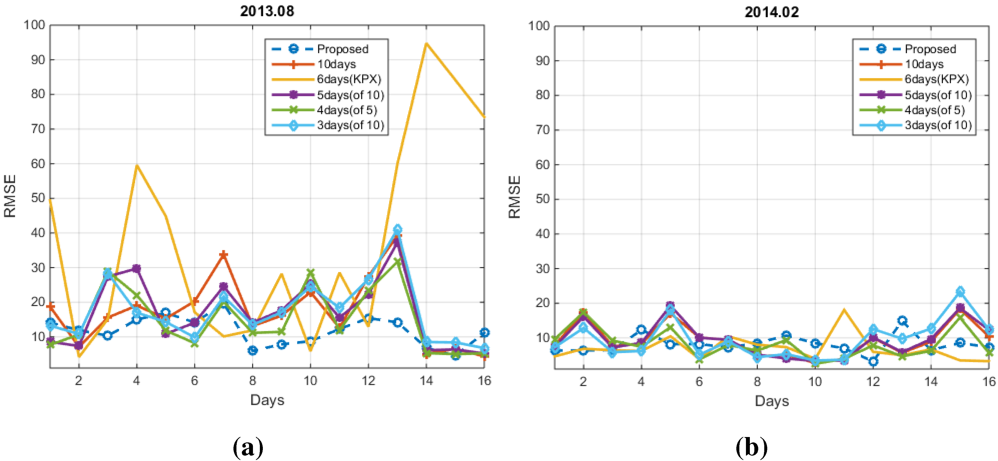
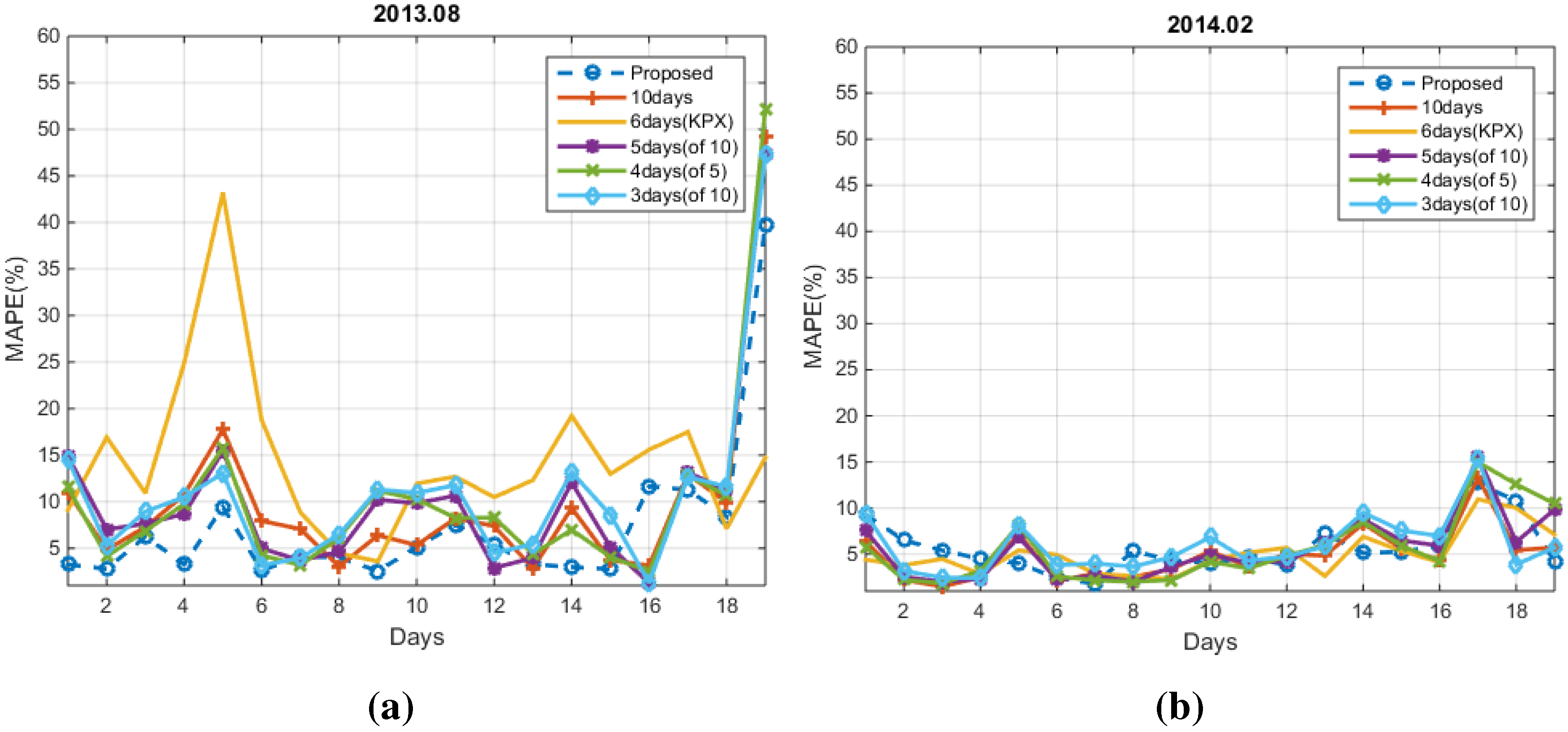
4. Experimental Results

In this section, we apply the above-mentioned methodology to the real data set. This section is organized as follows. At first, conventional methods with several variations are introduced. Then, the whole procedure to establish baseline is provided with numerical comparison.

4.1. Conventional Methods

It is generally accepted that the duration of approximately 10 days reasonably represents the expected consumption for normal operations. According to the report of the EnerNoc which develops DR resource in open market programs in North America [38], calculating baseline could be different depending on its purpose such as capacity, economic or ancillary services. In the resource capacity program, which is needed to ensure grid stability during the peak demand period, the preferred baseline calculation is to choose whole 10 non-event days or high 5 days out of 10 non-event days prior to DR event. This method is performed for each interval during the DR event:

$$bas{e}_5\left(h\right)=\frac{1}{5}\sum _{n=1}^5{P}_n\left(h\right)$$

(11)

where $P_n\left(h\right)$ is kWh energy consumption for n-th highest energy usage day at time h among previous 10 non-event days. Note that we will use $P_n\left(h\right)$ for other baselines estimations as well. In the economic program triggered by energy price signal, relatively short baseline window is used for calculation, namely, 5 non-event days and high 4 days out of 5 non-event days baseline window methods:

$$bas{e}_4\left(h\right)=\frac{1}{4}\sum _{n=1}^4{P}_n\left(h\right)$$

(12)

Another approach is to select high 3 days out of 10 non-event days which is also called Baseline Profile 3 (BLP3) method [39]. In this model, 3 days with the highest average load during the event period 12:00 PM–18:00 PM are selected from the previous 10 non-event days, and the average of the load over the three days is calculated for each hour such as:

$$bas{e}_3\left(h\right)=\frac{1}{3}\sum _{n=1}^3{P}_n\left(h\right)$$

(13)

After baseline method is applied, the adjustment factor is calculated as the difference between the observed demand and the estimated baseline. Applying the adjustment factor Δ could improve the accuracy of all baseline methodologies examined in DR participant’s building [39]. This factor is obtained by using two hours of consumption data before event start time denoted by $H_0$:

$$\Delta =\max \left(\frac{P(H_0-1)-bas{e}_M(H_0-1)+P(H_0-2)-bas{e}_M(H_0-2)}{2},0\right)$$

(14)

where $P\left(h\right)$ is kWh energy consumption of the event day, and $bas{e}_M$ means the baseline method with M window size as in Equations (11)–(13). The virtual power generated by DR with baseline M, denoted by $V_M$ is computed as the difference between baseline with the morning adjustment factor and real consumption until DR ending time denoted by $H_e$:

$$V_M=\sum _{h=H_0}^{H_e}\left(bas{e}_M\left(h\right)+\Delta -P\left(h\right)\right)$$

(15)

On the other hand, in the case of Korea market, instead of using the morning adjustment, moving average method is applied to 6 days after subtracting 2 high and 2 low days from previous 10 non-event days such as:

$$bas{e}_6\left(h\right)=\frac{1}{6}\sum _{n=1}^6{m}_n{\tilde{P}}_n\left(h\right)$$

(16)

where $m_1$ to $m_6$ are weights such as 0.25, 0.20, 0.15, 0.15, 0.15, and 0.10. ${\tilde{P}}_n\left(h\right)$ is the power consumption of n-th the most recent day from the event day. In this method, operators put more emphasis on the recent day’s energy consumption by assigning high weight.

4.2. Numerical Results

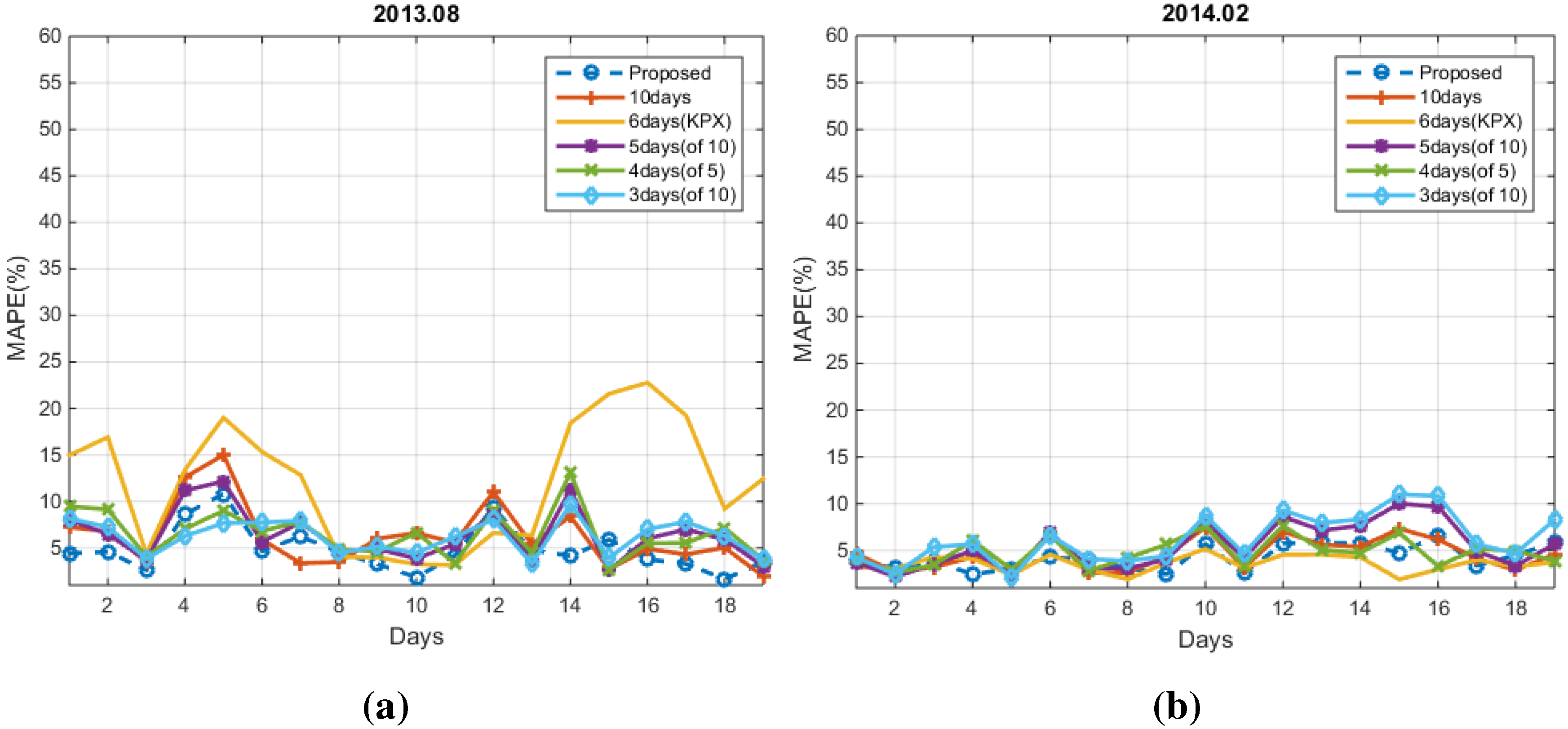
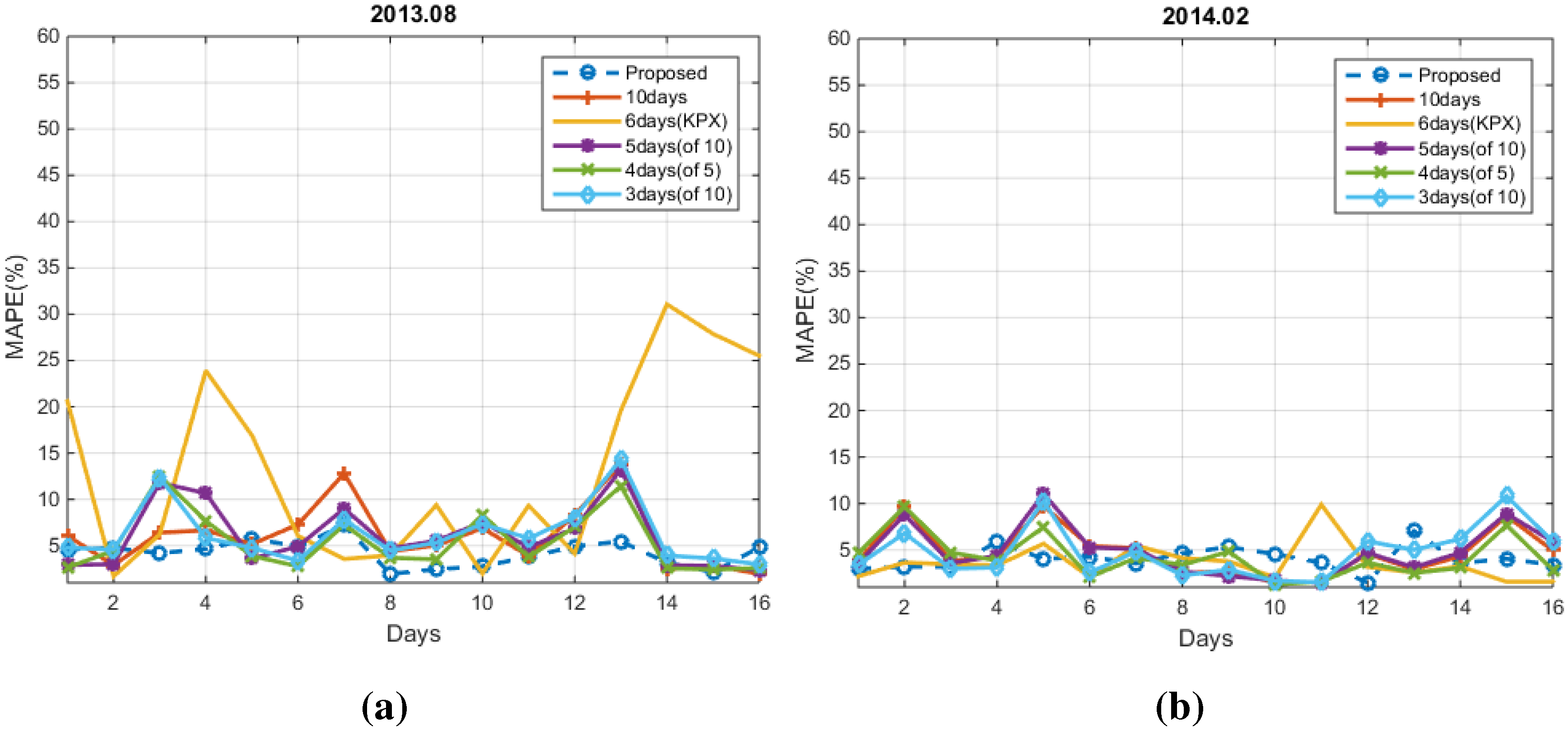
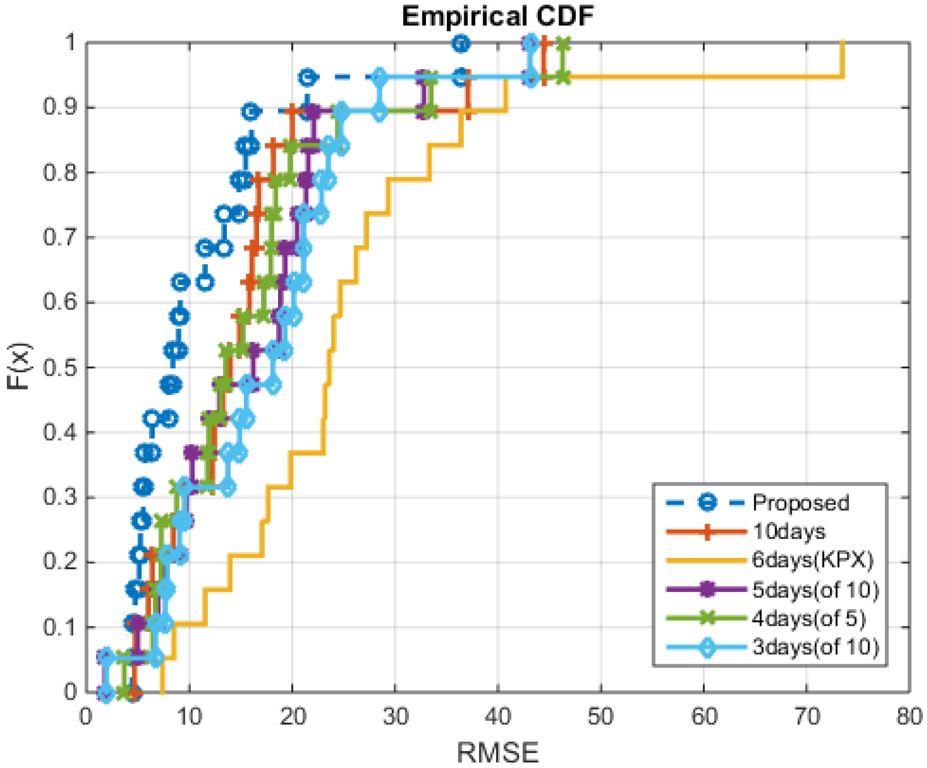
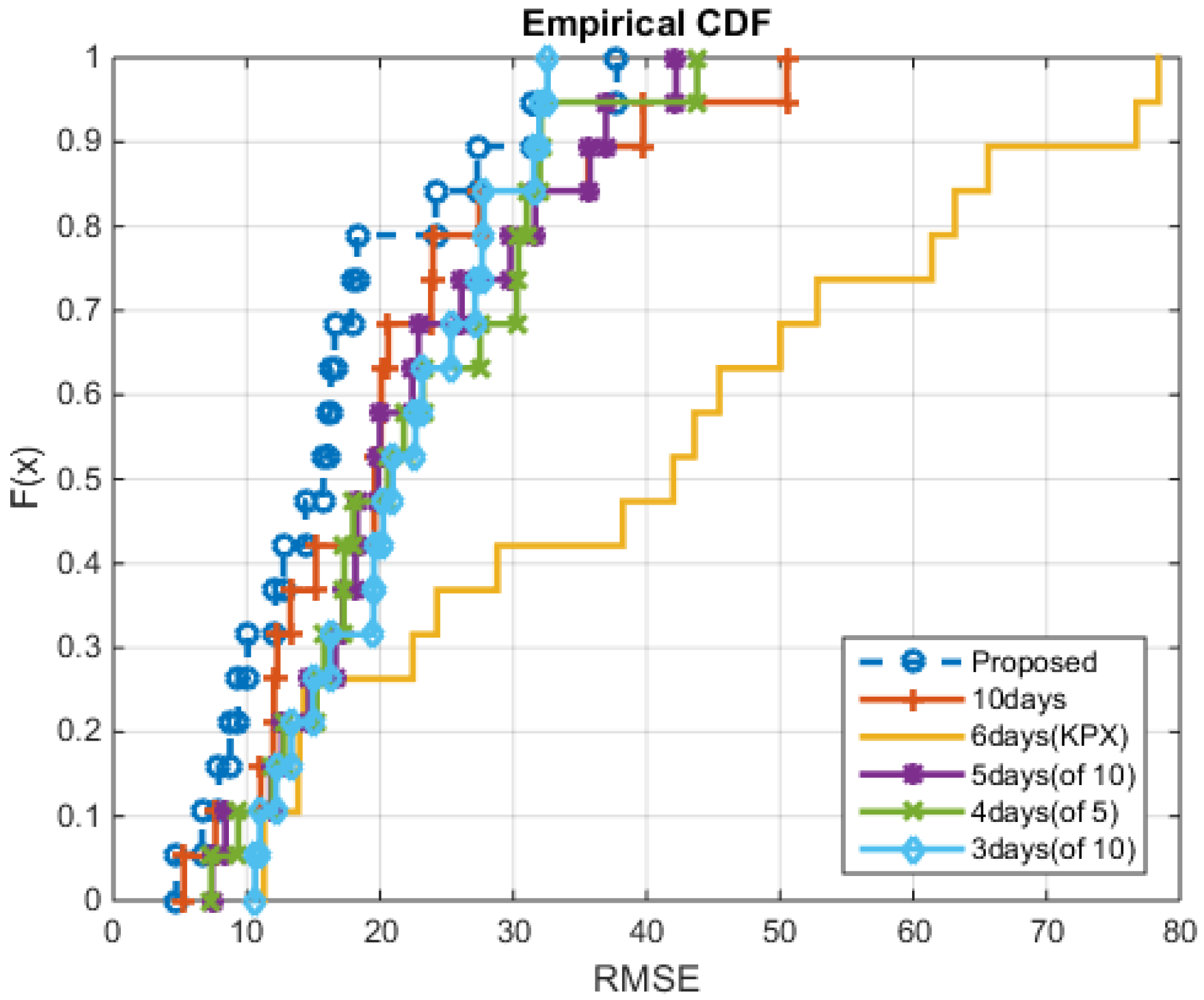
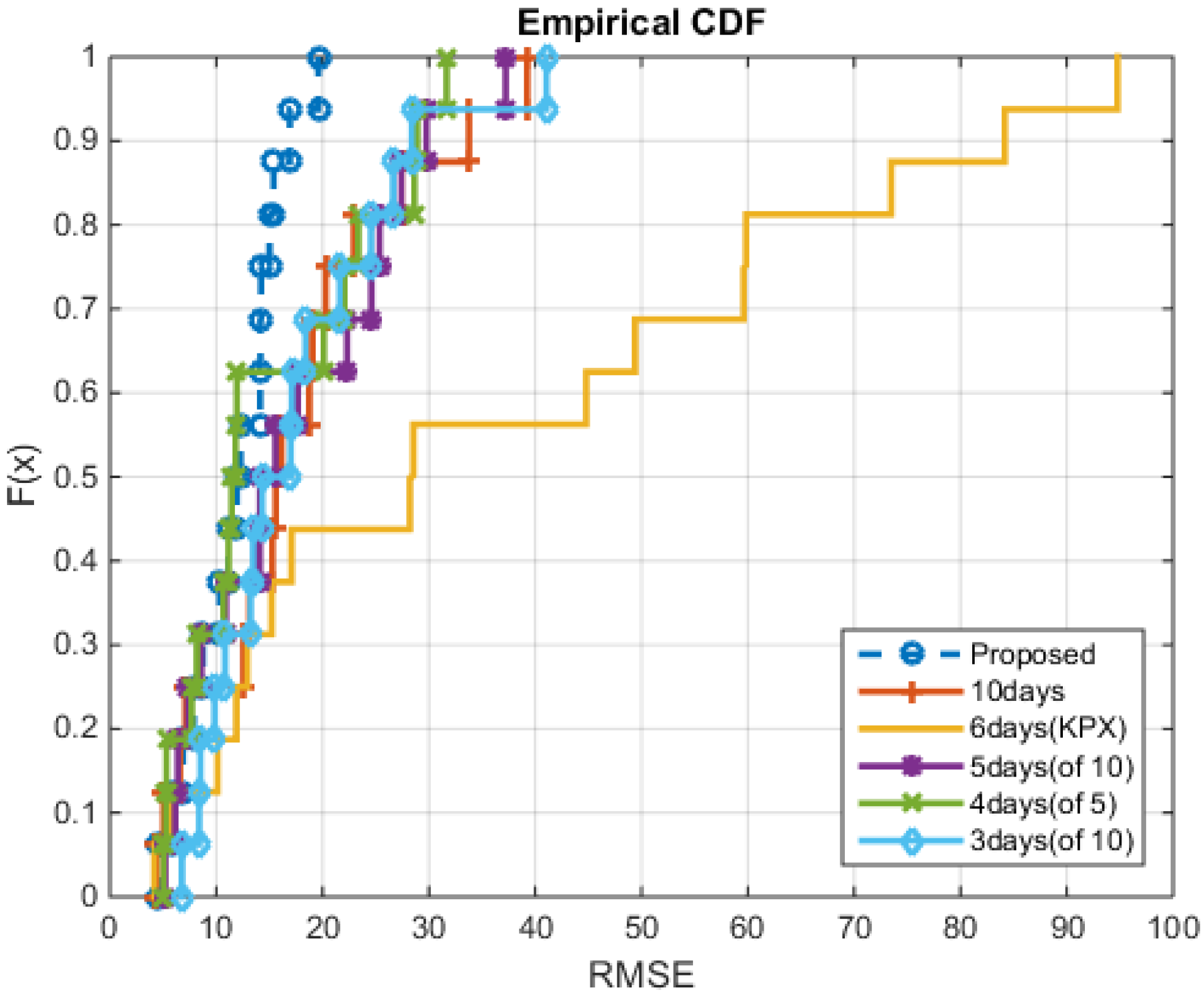
In this subsection, we demonstrate that proposed data-mining approach gives good guidelines to construct baseline in Korean residential buildings compared to conventional methods. As explained in the preceding sections, we test our method and other existing ones for each working day in a month.

We assume the DR event day happens in summer or winter because of high demand for air conditioning or heating. DR event usually occurs in the afternoon and lasts less than 6 h. Many reports state that DR usually starts between 1:00 PM and 2:00 PM by the rule of thumb [40]. To verify accuracy, we compare the real consumption and the estimated CBL. Two criteria commonly used to evaluate the accuracy of load estimation on DR event day are root mean square error (RMSE) and mean absolute percentage error (MAPE) [41] such as:

$$\mathrm{RMSE}=\sqrt{\frac{1}{H_e-H_0}{\displaystyle \sum _{h=H_0}^{H_e}}{(\widehat{P}\left(h\right)-P\left(h\right))}^2}$$

(17)

$$\mathrm{MAPE}=\frac{100}{H_e-H_0}\sum _{h=H_0}^{H_e}\frac{|\widehat{P}\left(h\right)-P\left(h\right)|}{P\left(h\right)}$$

(18)

where $H_e-H_0$ is DR event time intervals, $P\left(h\right),h=H_0,\dots ,H_e$ denotes the real electricity consumption, and $\widehat{P}\left(h\right),h=H_0,\dots ,H_e$ denotes the estimated CBL during DR event period.

In our experiment, the number of clusters is determined as follows. Though three combined indices were effective to determine the number of clusters in energy time series [33], we found that they have different impacts in our case. We evaluate three popular indices as can be seen in Figure 5, Figure 6 and Figure 7. We observe that the Dunn and Davies-Bouldin indices do not help us determine K since in both cases, as K grows, the clustering seems to get better. Recall that high Dunn index and low Davies-Bouldin index imply good clustering in general, but it does not hold in our case as they suggest that the number of cluster should be the number of the input data. Mean silhouette index, however, has a peak at some K, e.g., $K=21,27,16$ for each site A, B, and C, which serves for the number of clusters in our case. Each cluster corresponds to different consumption patterns of the customers. The representative load profiles are obtained by averaging load profiles in the same cluster. The created load profiles have distinct load shapes according to their consumption patterns in the morning. We test our approach to each working day in August, 2013 and February, 2014. Since DR could happen any working day depending on power system condition, we compare our methods and other existing ones in each working day independently. Assuming that DR starts at 1:00 PM with 6 h duration and the morning adjustment factor is calculated between 11:00 AM and 1:00 PM, we compute the RMSE and MAPE. Figure 8, Figure 9, Figure 10, Figure 11, Figure 12 and Figure 13 depict the obtained RMSE and MAPE values for three residential sites. Furthermore the empirical cumulative distribution function (CDF) of RMSE is plotted in Figure 14, Figure 15 and Figure 16 for comparing errors.

In overall, the proposed method shows more accurate load estimation compared to the five different types of the day matching methods. Specifically, Figure 8, Figure 9, Figure 10, Figure 11, Figure 12 and Figure 13 show that the proposed approach outperforms conventional approaches especially in the summer. This is because high energy consumption in the morning of summer affects positively on our proposed algorithm that tries to find similar patterns in the morning. In RMSE evaluation of the summer, our method has lower error rate, e.g., 20.9% to 68.5% in monthly average. In MAPE evaluation of the summer, our method has 21.9% to 68.1% lower error rate. The worst performance is observed for the case of 6-day method that does not apply the morning adjustment. When comparing the methods excluding 6-day method, our approach still achieves 20.9% to 37.7% and 22.0% to 33.3% lower error rate in terms of RMSE and MAPE, respectively. On the other hand, in the winter, both the proposed algorithm and day matching methods have adequately low error rates. This is because the power consumption in the morning does not affect the consumption during the day much, and thus clustering based on the morning consumption many not give additional benefit.

Figure 5. Validating the quality of the clusters produced by K-means algorithm in site A. (a) Dunn index (DI); (b) Davies-Bouldin index (DBI); (c) mean silhouette index (MSI).

Figure 5. Validating the quality of the clusters produced by K-means algorithm in site A. (a) Dunn index (DI); (b) Davies-Bouldin index (DBI); (c) mean silhouette index (MSI).

Figure 6. Validating the quality of the clusters produced by K-means algorithm in site B. (a) DI; (b) DBI; (c) MSI.

Figure 6. Validating the quality of the clusters produced by K-means algorithm in site B. (a) DI; (b) DBI; (c) MSI.

Figure 7. Validating the quality of the clusters produced by K-means algorithm in site C. (a) DI; (b) DBI; (c) MSI.

Figure 7. Validating the quality of the clusters produced by K-means algorithm in site C. (a) DI; (b) DBI; (c) MSI.

Figure 8. Root mean square error (RMSE) evaluation of site A in summer season (a) and winter season (b).

Figure 8. Root mean square error (RMSE) evaluation of site A in summer season (a) and winter season (b).

Figure 9. RMSE evaluation of site B in summer season (a) and winter season (b).

Figure 9. RMSE evaluation of site B in summer season (a) and winter season (b).

Figure 10. RMSE evaluation of site C in summer season (a) and winter season (b).

Figure 10. RMSE evaluation of site C in summer season (a) and winter season (b).

Figure 11. Mean absolute percentage error (MAPE) evaluation of site A in summer season (a) and winter season (b).

Figure 11. Mean absolute percentage error (MAPE) evaluation of site A in summer season (a) and winter season (b).

Figure 12. MAPE evaluation of site B in summer season (a) and winter season (b).

Figure 12. MAPE evaluation of site B in summer season (a) and winter season (b).

Figure 13. MAPE evaluation of site C in summer season (a) and winter season (b).

Figure 13. MAPE evaluation of site C in summer season (a) and winter season (b).

Figure 14. Cumulative distribution function (CDF) evaluation of the proposed models in site A.

Figure 14. Cumulative distribution function (CDF) evaluation of the proposed models in site A.

Figure 15. CDF evaluation of the proposed models in site B.

Figure 15. CDF evaluation of the proposed models in site B.

Figure 16. CDF evaluation of the proposed models in site C.

Figure 16. CDF evaluation of the proposed models in site C.

5. Conclusions

In this paper, we proposed a data-driven baseline load estimation of residential DR. Unlike the conventional techniques such as the day matching methods, we leveraged the data mining techniques, SOM and K-means clustering to find the days that are expected to have the most similar load patterns to the day of DR event. In SOM operation, the characteristic of large volume data is represented by weight vectors of units. Then we applied K-means clustering to group the days that have similar load patterns. In determining K, the number of clusters, we exploited the DI, DBI, and MSI. In the simulation, real residential electricity data in Korea is used to verify our proposed approach. The performance is evaluated based on RMSE and MAPE metrics which are widely adopted in error analysis. The results show significant lower error rates compared with the existing methods, especially in summer. Specifically, our approach outperforms current methods up to 68.5% lower error rate. Such noticeable results indicate that data-driven approach has great potential as a method for CBL estimation in DR management where large volume of smart metering data is being collected. As a substantial amount of electricity in residential buildings has been remained for DR resource, we expect that our proposed approach contributes to encouraging more people to participate in energy service.

References

1. Palensky, P.; Dietrich, D. Demand side management: Demand response, intelligent energy systems, and smart loads. IEEE Trans. Ind. Inform. 2011, 7, 381–388. [Google Scholar] [CrossRef]
2. Ruiz, N.; Cobelo, I.; Oyarzabal, J. A direct load control model for virtual power plant management. IEEE Trans. Power Syst. 2009, 24, 959–966. [Google Scholar] [CrossRef]
3. Goldberg, M.L.; Agnew, G.K. Measurement and Verification for Demand Response; U.S. Department of Energy: Washington, DC, USA, 2013. [Google Scholar]
4. Committee, A.L.R. Demand Response Measurement & Verification; Association of Edison Illuminating Companies: Birmingham, AL, USA, 2009. [Google Scholar]
5. Faria, P.; Vale, Z.; Antunes, P. Determining the adjustment baseline parameters to define an accurate customer baseline load. In Proceedings of the 2013 IEEE Power and Energy Society General Meeting (PES), Vancouver, BC, Canada, 21–25 July 2013; pp. 1–5.
6. The Demand Response Baseline; EnerNOC: Boston, MA, USA, 2011.
7. PJM Empirical Analysis of Demand Response Baseline Methods; KEMA, Inc.: Arnhem, The Netherlands, 2011.
8. Kim, J.; Nam, Y.; Hahn, T.; Hong, H. Demand Response Program Implementation Practices in Korea. In Proceedings of the 18th International Federation of Automatic Control (IFAC) World Congress, Milano, Italy, 28 August–2 September 2011; pp. 3704–3707.
9. Braithwait, S.; Hansen, D.; Armstrong, D. 2009 Load Impact Evaluation of California Statewide Critical-Peak Pricing Rates for Non-Residential Customers: Ex Post and Ex Ante Report; Christensen Associates Energy Consulting, LLC: Madison, WI, USA, 2010. [Google Scholar]
10. Iglesias, F.; Kastner, W. Analysis of similarity measures in times series clustering for the discovery of building energy patterns. Energies 2013, 6, 579–597. [Google Scholar] [CrossRef]
11. Amjady, N. Short-term hourly load forecasting using time-series modeling with peak load estimation capability. IEEE Trans. Power Syst. 2001, 16, 498–505. [Google Scholar] [CrossRef]
12. Chaouch, M. Clustering-based improvement of nonparametric functional time series forecasting: Application to intra-day household-level load curves. IEEE Trans. Smart Grid 2014, 5, 411–419. [Google Scholar] [CrossRef]
13. Hippert, H.S.; Pedreira, C.E.; Souza, R.C. Neural networks for short-term load forecasting: A review and evaluation. IEEE Trans. Power Syst. 2001, 16, 44–55. [Google Scholar] [CrossRef]
14. Pardo, A.; Meneu, V.; Valor, E. Temperature and seasonality influences on Spanish electricity load. Energy Econ. 2002, 24, 55–70. [Google Scholar] [CrossRef]
15. Bessec, M.; Fouquau, J. The non-linear link between electricity consumption and temperature in Europe: A threshold panel approach. Energy Econ. 2008, 30, 2705–2721. [Google Scholar] [CrossRef]
16. Tasdighi, M.; Ghasemi, H.; Rahimi-Kian, A. Residential microgrid scheduling based on smart meters data and temperature dependent thermal load modeling. IEEE Trans. Smart Grid 2014, 5, 349–357. [Google Scholar] [CrossRef]
17. Addy, N.; Mathieu, J.L.; Kiliccote, S.; Callaway, D.S. Understanding the effect of baseline modeling implementation choices on analysis of demand response performance. In Proceedings of the ASME 2012 International Mechanical Engineering Congress and Exposition, Houston, TX, USA, 9–15 November 2012; American Society of Mechanical Engineers: New York, NY, USA, 2012; pp. 133–141. [Google Scholar]
18. Coughlin, K.; Piette, M.A.; Goldman, C.; Kiliccote, S. Statistical analysis of baseline load models for non-residential buildings. Energy Build. 2009, 41, 374–381. [Google Scholar] [CrossRef]
19. Fayyad, U.M.; Piatetsky-Shapiro, G.; Smyth, P. From Data Mining to Knowledge Discovery: An Overview. In Advances in Knowledge Discovery and Data Mining; American Association for Artificial Intelligence: Menlo Park, CA, USA, 1996; pp. 1–34. [Google Scholar]
20. Figueiredo, V.; Rodrigues, F.; Vale, Z.; Gouveia, J.B. An electric energy consumer characterization framework based on data mining techniques. IEEE Trans. Power Syst. 2005, 20, 596–602. [Google Scholar] [CrossRef]
21. Ramos, S.; Duarte, J.M.; Duarte, F.J.; Vale, Z. A data-mining-based methodology to support MV electricity customers’ characterization. Energy Build. 2015, 91, 16–25. [Google Scholar] [CrossRef]
22. Valor, E.; Meneu, V.; Caselles, V. Daily air temperature and electricity load in Spain. J. Appl. Meteorol. 2001, 40, 1413–1421. [Google Scholar] [CrossRef]
23. Kohonen, T. Self-Organizing Maps; Springer: New York, NY, USA, 2001; Volume 30. [Google Scholar]
24. Rokach, L. A survey of clustering algorithms. In Data Mining and Knowledge Discovery Handbook; Springer: New York, NY, USA, 2010; pp. 269–298. [Google Scholar]
25. Huang, Z. Extensions to the k-means algorithm for clustering large data sets with categorical values. Data Min. Knowl. Discov. 1998, 2, 283–304. [Google Scholar] [CrossRef]
26. Abu-Mostafa, Y.S.; Magdon-Ismail, M.; Lin, H.T. Learning from Data; AMLBook: Berlin, Germany, 2012. [Google Scholar]
27. Vesanto, J.; Alhoniemi, E. Clustering of the self-organizing map. IEEE Trans. Neural Netw. 2000, 11, 586–600. [Google Scholar] [CrossRef] [PubMed]
28. Annual Energy Outlook; Energy Information Administration: Washington, DC, USA, 2015.
29. Woo, C.; Herter, K. Residential Demand Response Evaluation: A Scoping Study; Technical Report for Lawrence Berkeley National Laboratory: Berkeley, CA, USA, 2006. [Google Scholar]
30. Park, S.; Ryu, S.; Choi, Y.; Kim, H. A framework for baseline load estimation in demand response: Data mining approach. In Proceedings of the 2014 IEEE International Conference on Smart Grid Communications (SmartGridComm), Venice, Italy, 3–6 November 2014; pp. 638–643.
31. Vesanto, J.; Himberg, J.; Alhoniemi, E.; Parhankangas, J. Self-organizing map in Matlab: The SOM Toolbox. In Proceedings of the MATLAB Digital Signal Processing Conference, Espoo, Finland, 16–17 November 1999; Volume 99, pp. 16–17.
32. Xu, R.; Wunsch, D. Survey of clustering algorithms. IEEE Trans. Neural Netw. 2005, 16, 645–678. [Google Scholar] [CrossRef] [PubMed]
33. Martinez Alvarez, F.; Troncoso, A.; Riquelme, J.C.; Aguilar Ruiz, J.S. Energy time series forecasting based on pattern sequence similarity. IEEE Trans. Knowl. Data Eng. 2011, 23, 1230–1243. [Google Scholar] [CrossRef]
34. Dunn, J.C. A fuzzy relative of the ISODATA process and its use in detecting compact well-separated clusters. Cybern. Syst. 1973, 3, 32–57. [Google Scholar] [CrossRef]
35. Dunn, J.C. Well-separated clusters and optimal fuzzy partitions. J. Cybern. 1974, 4, 95–104. [Google Scholar] [CrossRef]
36. Davies, D.L.; Bouldin, D.W. A cluster separation measure. IEEE Trans. Pattern Anal. Mach. Intell. 1979, 1, 224–227. [Google Scholar] [CrossRef] [PubMed]
37. Rousseeuw, P.J. Silhouettes: A graphical aid to the interpretation and validation of cluster analysis. J. Comput. Appl. Math. 1987, 20, 53–65. [Google Scholar] [CrossRef]
38. Demand Response: A Multi-Purpose Resource For Utilities and Grid Operators; EnerNOC: Boston, MA, USA, 2009.
39. Coughlin, K.; Piette, M.A.; Goldman, C.; Kiliccote, S. Estimating Demand Response Load Impacts: Evaluation of Baseline Load Models for Non-Residential Buildings in California; Ernest Orlando Lawrence Berkeley National Laboratory: Berkeley, CA, USA, 2008. [Google Scholar]
40. Hurley, D.; Peterson, P.; Whited, M. Demand Response as a Power System Resource; Regulatory Assistance Project: Montpelier, VT, USA, 2013. [Google Scholar]
41. Li, G.; Liu, C.C.; Mattson, C.; Lawarree, J. Day-ahead electricity price forecasting in a grid environment. IEEE Trans. Power Syst. 2007, 22, 266–274. [Google Scholar] [CrossRef]