Abstract
This paper aims to analyse the economy-wide implications of a carbon tax applied on the Chilean electricity generation sector. In order to analyse the macroeconomic impacts, both an energy sectorial model and a Dynamic Stochastic General Equilibrium model have been used. During the year 2014 a carbon tax of 5 US$/tCO2e was approved in Chile. This tax and its increases (10, 20, 30, 40 and 50 US$/tCO2e) are evaluated in this article. The results show that the effectiveness of this policy depends on some variables which are not controlled by policy makers, for example, non-conventional renewable energy investment cost projections, natural gas prices, and the feasibility of exploiting hydroelectric resources. For a carbon tax of 20 US$/tCO2e, the average annual emission reduction would be between 1.1 and 9.1 million tCO2e. However, the price of the electricity would increase between 8.3 and 9.6 US$/MWh. This price shock would decrease the annual GDP growth rate by a maximum amount of 0.13%. This article compares this energy policy with others such as the introduction of non-conventional renewable energy sources and a sectorial cap. The results show that the same global greenhouse gas (GHG) emission reduction can be obtained with these policies, but the impact on the electricity price and GDP are lower than that of the carbon tax.
1. Introduction
Chile is a minor contributor to global greenhouse gas (GHG) emissions (0.2%). However, according to the last official GHG national inventory, the emissions from the energy sector have grown 101% between 1990 and 2010. Figure 1 shows the national inventory by sectors [1]. These statistics also show that the electricity generation sector is responsible for the highest amount of emissions. A recent study led by the government shows this situation has not changed. The electricity generation sector will continue to be the main GHG emitter, followed by the transport and industry sectors. These three sectors represent 77.2% of total emissions in 2013 [2].
Chile’s motivation to contribute to worldwide emissions reductions stems from the United Nations Framework Convention on Climate Change (UNFCCC) and its principle of common but differentiated responsibilities. The country intends to contribute to achieving the ultimate objective of the Convention by undertaking mitigation actions, as well as taking advantage of the potential environmental and social benefits and improvements in the quality of growth that can be directly derived from mitigation actions. Following this line of action, Chile will take nationally appropriate mitigation actions to achieve a 20% deviation below the “Business as Usual” emissions growth trajectory by 2020, as projected from the year 2007 according to Chile’s commitment at Copenhagen in 2010. During the last Climate Summit in New York in September 2014, the current president reaffirmed this voluntary commitment, subject to international support.
A more comprehensive analysis will help to establish exactly how Chile will fulfil its commitment to achieve its desired reduction in emissions. This paper aims to analyse the impact of a specific economic instrument: a carbon tax applied to the electricity generation sector. In 2014 Chile had a change of government following the presidential elections. The new government proposed a tributary reform which includes a carbon tax of 5 US$/tCO2 applied on fixed sources with installed capacity up to 50 MW (therefore, the carbon tax is not applied to the industry, transport, commercial, and residential sectors). A carbon tax would reduce the GHG emissions through two broad influences—a demand effect, reducing energy demand due to higher prices in the electricity sector as well as in the whole economy, and a substitution effect, that is switching from more to less carbon intensive fuels. The second effect is analysed in this paper. In addition, this instrument is compared with other energy policies such as an increase in non-conventional renewable energy sources and a cap on the total emissions of the electricity generation sector.
Figure 1.
Chilean national GHG inventory by sector [1]. The blue bar is the electricity generation sector which is analysed in this paper.
Carbon taxes have mostly been implemented in Scandinavian countries, Australia (it was abolished in 2014), and a few other European countries. Finland (1990), Sweden (1991), Norway (1991) and Denmark (1992) led the way in implementing a carbon tax [3].
Economic and energy models have been used in previous studies. Large-scale energy-economy models have been extensively used in the European Union (EU) climate and energy policies [4,5,6], and combining energy and economic models has been a standard in the EU. The link is necessary when sectorial models cannot provide all the answers that policy makers are looking for, for example, the impact on GDP pathway of an energy policy [7]. Most previous studies have used computable general equilibrium (CGE) models to analyse the economic implication of this kind of environmental policy. The GEM-E3 (a CGE model called General Equilibrium Model for Energy–Economy–Environment interactions) and the Energy–Environment–Economy macro-econometric (E3ME) model are being used to evaluate policy issues for the European Commission. These models are linked to the Price-Induced Market Equilibrium System (PRIMES) energy model [6]. In the Long Term Mitigation Scenario process [8,9] and in [10] a CGE model is used to evaluate the impact of a carbon tax in South Africa. In [11] the macroeconomic impact in Thailand of introducing an emission trading system and carbon capture storage technologies was evaluated. In [12,13] a CGE model is used to evaluate how a carbon tax policy impacts on energy consumption and GHG emissions in China. In [14] a multi-sector and multi-region CGE model is used to quantify the economic impacts of EU climate and energy package in Poland. In [15] two scenarios are evaluated to quantify the macroeconomic impacts in Pakistan, the first scenario only included different levels of carbon tax, and in the second scenario a carbon tax and energy efficiency improvements that have been jointly simulated are evaluated. Another approach is possible to find in [16], in this reference a Dynamic Stochastic General Equilibrium (DSGE) is developed to evaluate the macroeconomic impact of different mitigation action in Poland. In [17] an Input-Output matrix is used to estimate the short-term effects of a carbon tax in Italy, which includes the percentage increase in prices and the increase in the imports of commodities to substitute domestically produced ones as intermediate input.
Energy sectorial models have also been used in previous studies. TIMES (The Integrated MARKAL-EFOM System) Integrated Assessment Model (TIAM) is a bottom-up energy system model with a detailed description of different energy forms, resources, processing technologies and end-uses [18]. Model for Energy Supply Systems and their General Environmental impact (MESSAGE) is a supply energy model. Both models have been used by the Intergovernmental Panel on Climate Change (IPCC) to project global energy and emission scenarios. Also these models have been used to analyse local options with more details. For example, in [19] renewable energy options are analysed to mitigate climate change in India, and in [20] the MESSAGE model was used to evaluate 12 strategies to reduce the Malaysia’s carbon footprint of the energy sector. In [21] the Asian Pacific Integrated Model (AIM) is used for scenario analysis of GHG emission and the impacts of global warming in the Asian Pacific region. This model comprises 4 discrete models which are linked: The emission model and the global warning impact model are linked to two global physical models.
In [22] a fuzzy mixed-integer energy planning model under carbon tax policy is developed. In [23] an end-use energy model is presented for assessing policy options to reduce greenhouse gas emissions. This model evaluates the effects of imposing a carbon tax on various carbon emitting technologies in order to reduce CO2 emissions. In [24] the impact of renewable energy source incentives and mitigation policies (feed-in tariffs, quota obligation, emission trade, and carbon tax) are considered in the framework of the generation planning problem to be solved by a generation company. Renewable energy quota and emission limits result in a set of new constraints to be included in a traditional generation expansion planning model. In [25] an integrated power generation expansion planning model towards low-carbon economy is proposed. In [26] a short term optimization method is proposed to determine the optimal tax rate among generating units.
The literature review shows that macroeconomic models (CGE, DSGE, I/O matrix, etc.) do not represent endogenously all the details of the power sector to simulate the generation expansion planning under carbon tax scenarios. Due to this fact, in this paper both energy sectorial and macroeconomic models have been implemented, and an approach to link these two is presented. In [6] the GEM-E3 model cannot produce energy system simulations as accurately as the PRIMES model, therefore the GEM-E3 model is calibrated according to projections obtained by the PRIMES model [27]. The PRIMES model is more aggregated than engineering models and far more disaggregated than econometric models. Also in [6], the power generation mix was treated as exogenous in E3ME model and adapted to the results of the PRIMES model. In [14] a detailed bottom-up representation is used to model the electricity generation sector, however, this representation is less detailed in comparison to sectorial models. In [10] a long-term electricity investment plan of a previous study is used to calibrate a CGE multi-sectorial model. Also in [14] the power development plan is an input for the CGE model. In [28] a technological and the time period detail is introduced in a CGE framework to represent electricity demand and electricity generation by power plants. In a typical CGE model the energy sector is represented using one load block or stage per year. However, in this work [28] it was represented until 180 load blocks.
In this paper a DSGE model is selected instead of a CGE model. What DSGE and CGE modelling have in common is that they belong to the micro founded macroeconomic models of general equilibrium, but they differ in two important issues regarding modelling results: dynamics and uncertainty. DSGE models are strictly dynamic models, while CGE models are comparatively static ones. The dynamic characterization of the models allows for optimal decision rules that are not policy invariant, and where time is directly considered. This characterization has gained in terms of allowing analyses of the paths of the variables behavior instead of comparing different equilibriums, and by analysing the reachability of them, relative to the static characterization. The CGE type of model allows comparing steady state equilibriums but not the trajectories toward the equilibriums.
The treatment of uncertainty in the DSGE models makes them superior to CGE models, which are deterministic, because they allow a better fit of the theoretical models with the data. These features are causing a shift from CGE to DSGE modeling, which is becoming a valuable tool for assessing policy analysis, mechanisms analysis and projections [29,30]. However, the CGE models include a large variety of sectors, so they make possible to analyze sectoral composition of output, employment, capital, etc., while the DSGE models focus in more aggregated analysis.
In Chile there are two main independent power systems, the Central Interconnected System (in Spanish, Sistema Interconectado Central, SIC), and the Norte Grande Interconnected System (in Spanish, Sistema Interconectado del Norte Grande, SING). Figure 2 and Figure 3 show the historical generation by source for the SIC and SING, respectively. The hydroelectricity generation is one of the main sources in the SIC, whereas in the SING coal is one of the main energy sources. The maximum demand in SIC was 7,535 MW and SING was 2,300 MW in 2014.
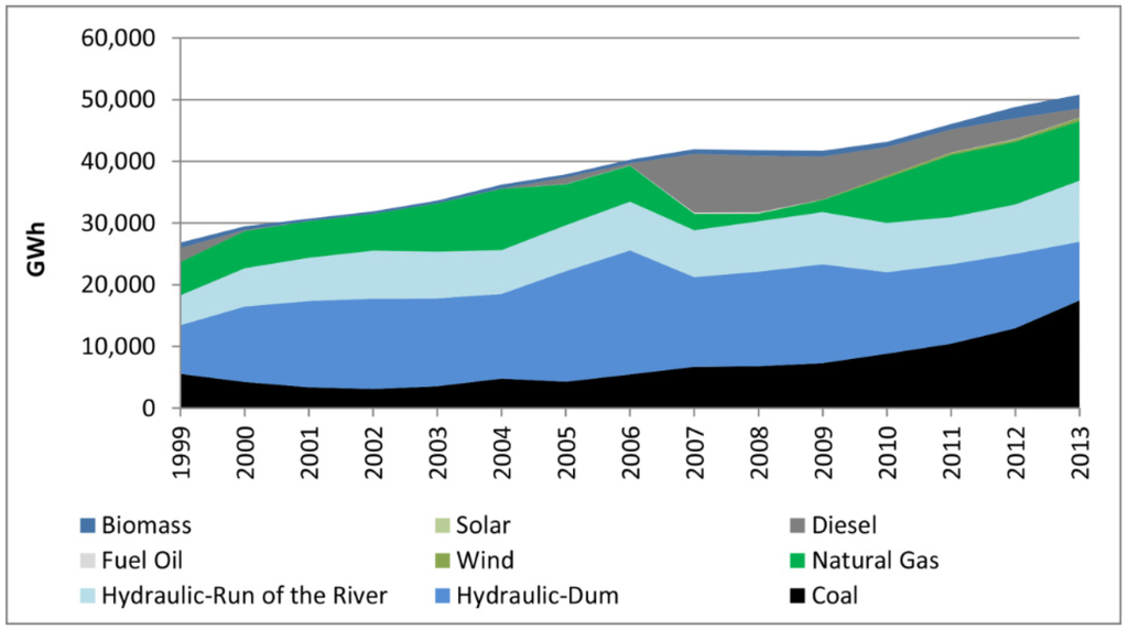
Figure 2.
Electricity generation by sources, SIC 1999–2013.
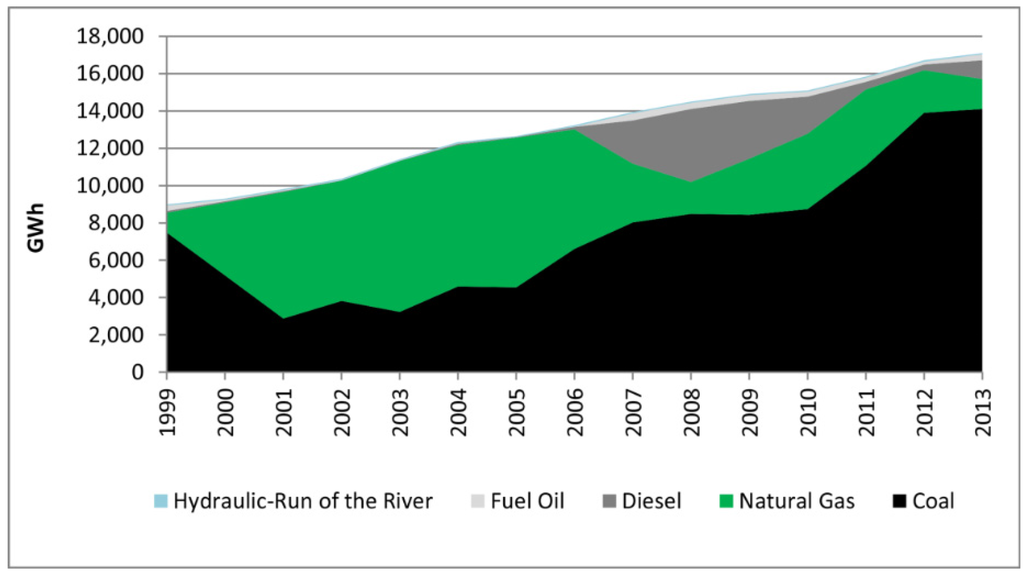
Figure 3.
Electricity generation by sources, SING 1999–2013.
Chile has great potential to produce electricity with renewable energy sources, such as hydroelectric (12,000 MW), solar (1,000,000 MW), wind (40,000 MW) and geothermal (16,000 MW) sources [31]. However, some issues have affected the development of this technology in Chile. In the case of solar and wind energy, there is uncertainty related to the evolution of the future investment cost and the lack of access to long term contracts constitutes a barrier for project developments. In the case of hydroelectric sources, environmental problems have faced some projects. For example, the hydroelectric generation potential of the Aysén region has been estimated to be more than 7,000 MW. Two specific projects have been evaluated in this zone: HidroAysen (2,750 MW) and Cuervo (640 MW). However, these projects have faced the opposition of several groups due to the fact that these would be installed in a pristine region of Patagonia, known for glaciers and lakes. In addition, these projects require a transmission line of more than 2,000 km to inject its energy to SIC power system. The first project presented its environmental evaluation in year 2008, and was approved in May of 2011. However an action complaint against the environmental resolution was presented which had to be resolved by a Minister Committee. The final resolution of this was extended for more than three years. Finally, the environmental evaluation was rejected by the current Minister Committee, and it is not clear if the company will present the environmental evaluation again. The environmental evaluation of the transmission line has not been presented yet.
Figure 2 and Figure 3 show that natural gas was one of the main energy sources between 2000 and 2006. Most of the natural gas was imported from Argentina, however this supply experienced many shortfalls. To overcome this energy problem in Chile, two Liquid Natural Gas (LNG) terminals were built: Mejillones and Quintero. The first began to operate in 2009. However, it is currently operating below its maximum capacity due to the high price of LNG in comparison to electricity generation from coal (see Figure 3). In the case of the Quintero LNG terminal, it is operating at full capacity. Four companies share ownership of this terminal: British Gas; the National Petroleum Company of Chile (ENAP), which is a state refiner; Chilean Distributor for Natural Gas for Metropolitan Region (METROGAS), and National Electricity Company (ENDESA), which is one of the biggest private electricity generation companies in Chile. Apart from ENDESA, there are other companies which have natural gas power plants (for example Nehuenco (785 MW) and Nueva Renca (305 MW)), however, these do not have open access to the terminal. At times METROGAS or ENAP have sold gas surpluses to these companies, but at a high price. There are uncertainties about access to the terminal to get gas at competitive prices or the access using their own terminal.
To evaluate the above uncertainties, a sensitivity analysis is proposed to manage the following aspects: solar photovoltaic technology investment cost, projection for LNG prices, and potential use of hydroelectric resources in the extreme south of Chile. Different baseline scenarios are built considering these variables. Other uncertain sources could be included in this analysis but the focus of this work has been limited to these in order to show the impact on the projection of GHG emission reduction and macroeconomic results.
The main contributions of this paper are: to analyse the impact of the carbon tax at the Chilean electricity sector using both a sectorial model and a DSGE model. A novel approach is proposed to integrate results from the sectorial model and a DSGE model. This work shows that the effectiveness of reducing GHG emission depends on some variables which could not be controlled by policy makers. Finally, the carbon tax is compared to other energy policies and interesting results are found.
2. Methodology
2.1. Overview Description
Figure 4 shows an overview of the approach to evaluate the carbon tax. A generation expansion planning model is developed to project the installed capacity and electricity generation for the period 2013–2030. The models for industry, transport and commercial, public and residential (CPR) sectors project the electricity demand which is an input for the generation expansion planning model. In this iteration, the sectorial models are run considering a base value for the GDP projection and considering a carbon tax applied to the electricity generation sector. The electricity price obtained from the electricity generation sector, expressed at constant prices, is an input for the DSGE model. The new electricity price projection is introduced in the DSGE model as a price shock. Then, the DSGE model will estimate the effects on GDP path due to the electricity price shock.
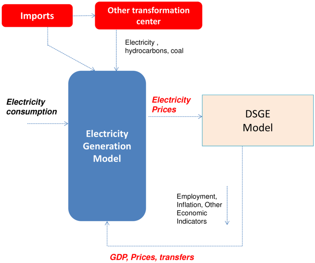
Figure 4.
General description of the Chilean approach. The price of the electricity is output of the sectorial model and is an input for the DSGE model.
The DSGE model, as its name indicates, is a general equilibrium model, which means that it takes into account all interactions occurring among all the economic agents, who adjust their decisions according to changes in relative prices. Under this framework, an increase in the relative price of electricity encourages firms to substitute from electricity toward capital and labour, given the technological possibilities, making the electricity demand in the DSGE endogenous. However, this substitution is not perfect, but rather limited, given the complementarity of energy with capital and labour which negatively affects production possibilities. After the energy prices rise, the economy must move to a new long-run equilibrium, with lower growth rates during the period of convergence. The size and number of periods of lower GDP growth rates during the transition period will depend on how big the increase in the electricity price due to the carbon tax is and how fast the tax is implemented. If it is slightly and gradual, the GDP growth rate will be affected for a short time and not significantly. Conversely, if the rise in the tax is stronger the GDP growth rate will be strongly affected and for longer periods of time. When the economy gets back to the equilibrium, it will grow at rates similar to those before the imposition of the tax rates. This is thanks to the exogenous improvements in productivity and population growth. However, this growth will be based on a lower level, due to lower growth rates occurred in the transition period. This will result in a permanent deviation of the GDP level regard the baseline level (without tax). The approach proposed considers an iteration procedure, where the new path of GDP is introduced into the sectoral models in order to estimate again a new lower electricity demand. It is expected that with a lower demand, the emission projection would reduce, as it is analysed in [32].
A limitation of this approach should be recognized. The literature review shows that both CGE and DSGE models represent in a simplified manner the productive sectors of the economy. In particular our DSGE model does not explicitly include an electricity generation sector; the electricity sector works as an imported commodity which is sold to the economy at the prices given by the linkage with the electricity generation sectorial model. In this context, electricity is the only energy factor included in the DSGE model, which implies that the firms are not able to substitute electricity with another type of fuel when they face electricity price increases. In this context, it is possible that the results might slightly overestimate the negative impact on GDP growth rate due to the implementation of a carbon tax.
2.2. Generation Expansion Planning Model
The objective of this model is to determine the optimal combination of power generation to meet the projected demand for the time horizon 2013–2030. We formulate the problem as if planning was matched by a central or state government. The objective function is to minimize the capital costs in new plants, the variable cost related to fuel consumption, variable cost associated to non-fuel consumption, and the cost of unserved energy. In addition, the objective function includes a penalty for the GHG emitted emissions:
where the optimization problem variables (MW) is the additional installed capacity by year, and (MWh) is the electricity generation in the stage s and load block b of the year t. Every year is divide into monthly (12) stages, and every stage is represented by five load blocks (the load duration curve is divided into five blocks). is the duration of the load block b. is the capital cost annuity (US$/MW), is the variable cost (fuel and non-fuel cost) (US$/MWh), (ton CO2/MWh) is the emission factor for each kind of technology, (US$/ton CO2) is the carbon tax and r is the private discount rate (10%). The factor will take the amount of 5, 10, 20, 30, 40, and 50 US$/tCO2e between 2017 and 2030. The problem is subject to the following constraints:
- ◾
- Energy balance between the electricity generations and demand. A multi-nodal formulation is used to represent the interconnection between SIC and SING. The electricity demand is exogenous in this model.
- ◾
- Upper and lower bounds on the electricity generation of power plants.
- ◾
- Maximum feasible amount of investment for each kind of technology that could happen in a year.
- ◾
- Maximum feasible amount of investment for each kind of technology for the total period. The potential installed capacity for hydroelectric run-of-river power plants is set according potential projects which are currently under evaluation. In the case of geothermal energy, a conservative expectative is assumed in comparison with previous works in Chile [33].
- ◾
- Quota obligation to renewable energy generation according to new renewable energy law (20% by 2025).
- ◾
- Technical parameters of the electricity generation plants were obtained from the ISO webpages of SIC [34] and SING [35]. The model represents 290 power plants.
- ◾
- Information regarding power plants which are being built was collected from reports published by the National Regulatory Institution [36,37].
- ◾
- Hydroelectric-dam plants can regulate their generation during every stage. On the other hand, hydraulic-run of river and small hydroelectric plants are not able to regulate their energy generation.
- ◾
- Minimum technical power is considered for coal and LNG power plants. This constraint avoids starts up and shut down between blocks in the same stage. This constraint is included to avoid infeasible solutions when high penetration of non-conventional renewable energy sources with an intermitted generation (e.g., solar and wind generation) is introduced to the power system.
- ◾
- Minimum sizes for new power plants are considered. The minimum size for a coal, natural gas, and hydroelectric power plant were 250 MW, 200 MW and 100 MW, respectively.
- ◾
- Investment costs for the first year were obtained from [36,37]. The cost projection is based on growth rate used in [33]. The investment costs projection used in this work are in the Appendix.
- ◾
- Currently there is transmission project that will connect the two main power systems of Chile (SINC and SING). It is supposed that the interconnection between SIC and SING will happen by the year 2019.
- ◾
- The baseline scenario does not consider nuclear energy as an energy option.
2.3. Macroeconomic Model
A DSGE model calibrated for the Chilean economy is used for this exercise. This model is based on a previous work by Medina and Soto [38,39]. Figure 5 represents the structure of the main agents involved in the model.
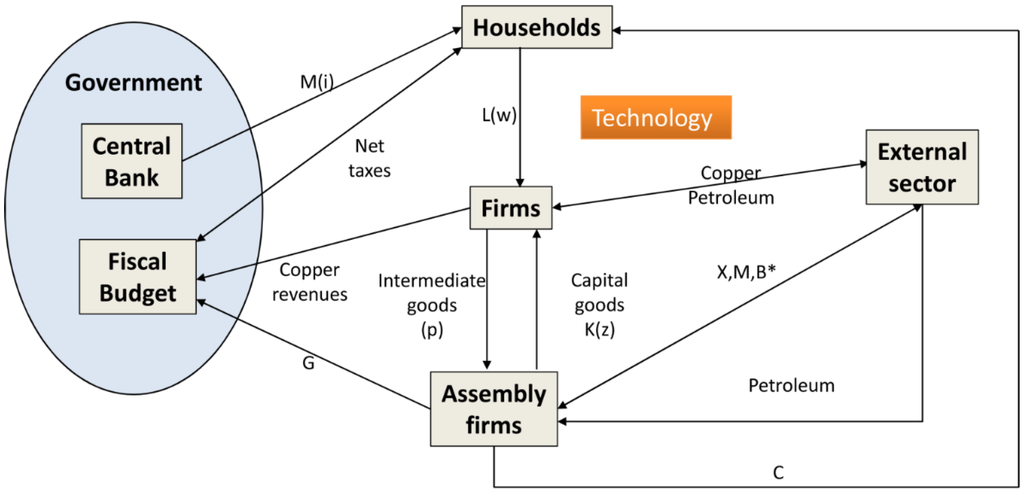
Figure 5.
General description of DSGE model.
There is a continuum of households and different types of firms in the economy. Households live infinitely, take decisions on consumption and savings, and set wages in a staggered way. There is a set of firms that produce differentiated varieties of tradable intermediate goods using labour and capital. They have monopoly power over the varieties they produce and set prices in a staggered way. Another set of firms are importers that distribute domestically different varieties of foreign intermediate varieties. These firms have monopoly power over the varieties they distribute, and also set prices in a staggered fashion. Setting wages and prices in a staggered way to the equilibrium price is an assumption used by previous macroeconomic literature [40,41,42] which implies introducing of prices rigidities in order to model the gradual adjustment of the economy to shocks. These firms have monopoly power over the varieties they distribute, and also set prices in a staggered fashion. There is a third single firm that produces a commodity good which is completely exported abroad. This firm has no market power in the international market price. Production by this firm is exogenously determined and requires no inputs. Its revenues are owned by the government and by foreign investors. Domestic and foreign intermediate varieties are used to assemble two final goods: home and foreign goods. Electricity is included in the foreign goods, which is sold in the domestic economy at a given price determined by the exogenous electricity generation model. These two final goods are combined into a bundle consumed by households, another bundle consumed by the government and a third bundle that corresponds to new capital goods that are accumulated to increase the capital stock.
A previous DSGE model [38] for the Chilean economy was adapted in this paper. The optimization problem of the firms consists in maximizing the total income less the cost:
where Y is the production of the firm, K is the capital, L is number of employees, E is the electricity consumption of the firm, is the price of the production, is the salary, is the price of the capital, and is the price of the electricity. The production function can be expressed as:
The elasticity ε was calibrated by using the historical data of the National Energy Balance from 1990 to 2012. An energy price index is estimated using historical data of fossil fuel primary sources (coal, diesel, and natural gas):
In the last equation is the total energy from fossil fuels sources resulting from the sum of each “j” energy source weighted by of their relative prices (). The elasticity of substitution ε is calibrated using historical data of . This is a strong assumption, which means that the only energy input used in the economy is electricity. This assumption allows estimating with the DSGE model the effect of the carbon tax imposed using the electricity generation model.
Moreover, the share of the energy by the total output of the economy would be modified with the productivity according the indirect productivity of the expenditure of energy by output . The electricity price obtained from the electricity generation sector for these different scenarios is an input for the DSGE model. The following expression is used to calculate the increase in the price of electricity ():
where corresponds to the present value of the variation of the capital expenditure (first term of objective function in the Equation (1)) in power plants in comparison with the baseline scenario, i.e., the case without carbon tax; represents the variation of the operation expenditure (second term of objective function in the Equation (1)), TAX is the carbon tax that the generation companies should pay due to their GHG emissions (third term of objective function in the Equation (1)), is the total electricity generation in the year t, tini is the starting year for the carbon tax application. , , and TAX are outputs of the electricity generation model. Finally, r is the private discount rate used in the electricity generation sector. It is assumed that the cost that electricity generation companies will pay due to the carbon tax will be transferred to their customers. The discount rate used in that equation the private discount rate and it is equal to 10%. This is the typical discount rate used in the Chilean electricity sector which it is a near 100% a private sector. For example, the regulation of the transmission system states that the annuity of the transmission asset is calculated with a discount rate of 10%. Also, the electricity distribution regulation states a discount rate of 10% to calculate the annuity of the investments. Consequently, the selected discount rate intends reflecting the decision dynamic of the electricity. This approach implies a constant and permanent increase in the electricity price after the carbon tax is imposed.
The price of electricity in the DSGE model presents the following autoregressive process of order 1:
Equation (6) works as the linkage between the electricity generation sectoral model and the DSGE. This structure allows introducing the increase of electricity price resulting from the sectoral model into the DSGE model as an electricity price shock.
The variance of the normal distribution () is calibrated according to the historical data of electricity prices. The simulation procedure seeks to replicate the new exogenous path of electricity prices, with a permanent increase due to carbon tax, using the shock of Equation (6) to mimic this effect. More details of the model can be found in [38,39]. After changing energy prices the economy must move to a new long-run equilibrium. The resulting steady state will show a shift in the growth rates during the convergence period. Upon reaching the new steady state the economy will grow at similar rates before imposing the tax because of the improvements in productivity and population growth, but this growth will result in a lower GDP level due to lower growth rates in the transition period.
Regarding the implementation of the proposed analysis framework, the generation expansion planning model was programmed in MATHPROG using a GLPK distribution [43] and solved by CPLEX MIP solver [44]. The DSGE model was programmed using DYNARE and MATLAB [45]. The MIP problems were solved with a gap below 0.03%.
3. Case Study
The impacts of a carbon tax on the Chilean electricity generation sector are evaluated considering six levels: 5, 10, 20, 30, 40, and 50 US$/tCO2e. The carbon tax is applied between 2017 and 2030 to both the SING and SIC power systems. For this exercise a simplification of the framework explained in Section 2 will be used. In particular, there will be no iteration process from the new GDP path estimated by the DSGE to the electricity generation model. Due to the lack of specific information, scenarios with gradual carbon tax rate increases are not explored. Nevertheless, the effect of any gradual implementation scheme should be within the observed overall simulation results.
For this simulation exercise several assumptions are made. An annual exogenous growth rate of 1.5% and 1.0% for productivity and employment is assumed, respectively. For every scenario we assume that the convergence time of electricity prices to the new equilibrium is 12 quarters and gradual increases will be linear. The current price of the original steady state energy is 105 US$/MWh. This price does not include the distribution cost.
A sensitivity analysis is performed for three main parameters which are inputs for the optimization problem (the reason for selecting these parameters was discussed in the Introduction Section): projection of investment cost in solar photovoltaic (PV) technology, projection for LNG prices, and potential use of hydroelectric resource in the extreme south of Chile, see Table 1. Considering these uncertainties four scenarios are projected (see Table 2). We define these scenarios as baseline scenarios.

Table 1.
Sensitivity analyses considering three sources of uncertainties.
| Solar Investment Cost | LNG Prices | Hydroelectric Resources in the Extreme South of Chile |
|---|---|---|
| Case 1: Base situation | Case 1: Base situation | Case 1: No exploitation of additional hydroelectric resources. |
| Case 2: More optimistic projection of solar investment cost, see Annex | Case 2: More optimistic LNG prices projection for power plants which have not open access to LNG terminal, see Annex | Case 2: An additional potential of 2,750 MW of hydroelectric source is considered. |
Table 2.
Evaluated scenarios built from the sources of uncertainties. These scenarios are called baseline scenarios.
| Scenario “S” or Baseline Scenarios | Solar Investment cost | LNG Prices | Exploit the Hydroelectric Resource in the Extreme South of Chile |
|---|---|---|---|
| S1 (Baseline #1): Moderate Scenario in terms of the development of solar investment cost projection and LNG price. This scenario does not consider the development of big hydroelectric projects in the south of Chile. | Case 1 | Case 1 | Case 1 |
| S2 (Baseline #2): Equal to scenario 1 but more optimistic regarding the solar investment cost projection. | Case 2 | Case 1 | Case 1 |
| S3 (Baseline #3): Equal to scenario 1 but it considers the development of big hydroelectric projects in the south of Chile. | Case 1 | Case 1 | Case 2 |
| S4 (Baseline #4): Equal to scenario 1 but more optimistic regarding the projection of LNG prices. | Case 1 | Case 2 | Case 1 |
3.1. Electricity Generation Sector Results
Figure 6 shows the GHG trajectory for the scenarios defined in Table 2. These scenarios are the four baseline scenarios defined above (without carbon tax). The carbon tax is applied in every one of these four scenarios. Figure 6 shows that the GHG trajectories are different due to the different assumptions defined in Table 2. For example, the GHG emissions of Baseline #3 begin to fall from the year 2022 in comparison to the other baseline scenarios. In this case it is supposed that the hydroelectric generation potential of the Aysén region will be available from 2022. The planning expansion solution obtained from the optimization model shows that 2,750 MW would be installed between 2022 and 2026. This hydroelectric potential is not available in the other baselines scenarios (see Table 1 and Table 2). The electricity generation of hydroelectric power plants depends on the hydrological conditions. In the model used in this paper a hydrological trend based on historical series, is supposed. It means that, in the future, some years will be wet, others will be dry, and others will be normal. It explains some ups and downs in the GHG emissions. For example, in the year 2024, the GHG emissions grow due to the fact that this year is wetter than previous years. All the baselines scenarios were evaluated with the same hydrological trend.
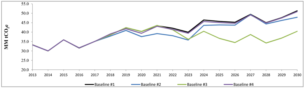
Figure 6.
GHG trajectory for different baseline scenarios (MM = million).
Figure 7, Figure 8, Figure 9 and Figure 10 show the total GHG emissions (SING and SIC) for the baseline scenarios, in comparison to different carbon tax levels (5‒50 US$/tCO2e). The results show that the emission trajectory depends on the evaluated baseline scenario. In Scenario #1, from the year 2023 the results show a big difference between a tax of 30 and 40 US$/tCO2. This is due to the fact that when the carbon tax of 40 US$/tCO2 is applied the coal technology is less competitive in comparison to the next cheapest technology, in this case, solar energy. In 2023, the Levelized Cost of Energy (LCE) of coal technology without carbon tax is 84 US$/MWh, and with a carbon tax of 10, 20, 30, and 40 US$/tCO2 are 92, 101, 109, and 118 US$/MWh, respectively, while the LCE of solar technology is 110 US$/MWh. Therefore, with a carbon tax of 40 US$/tCO2e the solar technology is cheaper than coal technology, and then there are less GHG emissions. However, note that with a carbon tax of 30 US$/tCO2e the difference is very small. Probably a value higher than 30 and lower 40 would have the same result. This is the reason why in Scenario #2 (in this case the solar investment cost is more optimistic) the carbon tax of 30 US$/tCO2e has a major impact. It is important to emphasize that the methodology used an optimization problem with technical constraints of the system operation to project the investment in new power plant, but, by simplification, we have calculated the LCE to give an explanation of the big difference between 30 and 40 US$/tCO2e.
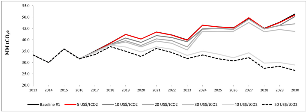
Figure 7.
Emissions for baseline scenario #1 in comparison to different scenarios of carbon tax (MM = million).
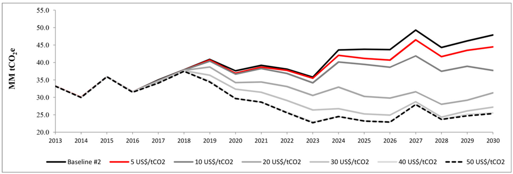
Figure 8.
Emissions for baseline scenario #2 in comparison to different scenarios of carbon tax (MM = million).
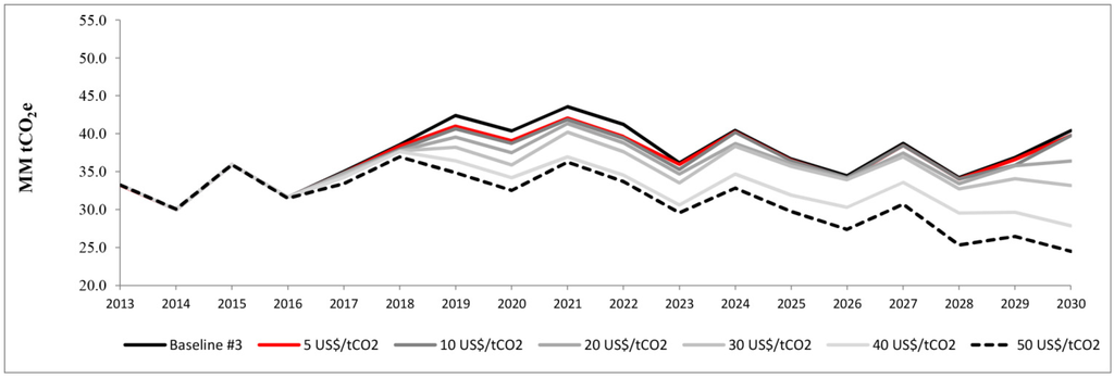
Figure 9.
Emissions for baseline scenario #3 in comparison to different scenarios of carbon tax (MM = million).
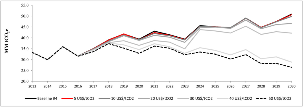
Figure 10.
Emissions for baseline scenario #4 in comparison to different scenarios of carbon tax (MM = million).
In addition, different indicators are proposed to compare the impact of the carbon tax on the electricity generation sector with the baseline scenario: OPEX, CAPEX, and carbon tax revenue. These indicators are expressed in present value and as deviation with respect to the baseline scenario. The carbon tax revenue is the sum of the whole period. All the monetary values are expressed in constant prices. Also cumulative emission reduction, annual average emission reduction, and average increase of the electricity price at the national level are reported (see Table 3). The average increase of the electricity price is calculated using Equation (5) and it is an output of the sectorial model. It is supposed that the average increase of the price will be constant between 2017 and 2030.
Table 3.
Resulting indicators to assess the impact of the carbon tax on the electricity generation sector. These indicators are expressed in present value and as deviation with respect baseline scenario. The negative values mean a reduction with respect to baseline scenario (MM = million). OPEX, operational expenditure; CAPEX, capital expenditure.
| Unit Scenario | Carbon tax | ∆ OPEX | Carbon tax revenue | ∆ CAPEX | Cumulative ∆ emission | Average ∆ Annual Emission | ∆ Electricity Price |
|---|---|---|---|---|---|---|---|
| US$/tCO2 | MM US$ | MM US$ | MM US$ | MM tCO2e | MM tCO2e | US$/MWh | |
| S1 | 5 | −58.3 | 1168.8 | 57.8 | −1.1 | −0.1 | 2.1 |
| 10 | −136.9 | 2288.3 | 178.9 | −13.4 | −1.0 | 4.2 | |
| 20 | −644.1 | 4488.0 | 765.5 | −25.0 | −1.8 | 8.2 | |
| 30 | −970.5 | 6581.5 | 1226.8 | −40.9 | −2.9 | 12.2 | |
| 40 | −2039.0 | 7644.0 | 3314.3 | −139.8 | −10.0 | 15.9 | |
| 50 | −2906.1 | 9147.4 | 4564.2 | −162.4 | −11.6 | 19.3 | |
| S2 | 5 | −407.1 | 1085.5 | 430.9 | −19.5 | −1.4 | 2.0 |
| 10 | −762.8 | 2109.8 | 837.5 | −43.6 | −3.1 | 3.9 | |
| 20 | −1807.3 | 3748.9 | 2228.8 | −118.9 | −8.5 | 7.5 | |
| 30 | −2681.2 | 5328.4 | 3349.2 | −150.3 | −10.7 | 10.7 | |
| 40 | −126.9 | 6815.3 | 4051.9 | −170.5 | −12.2 | 13.8 | |
| 50 | −3692.1 | 8043.6 | 5044.7 | −195.3 | −13.9 | 16.8 | |
| S3 | 5 | −81.2 | 1054.0 | 93.6 | −7.9 | −0.6 | 1.9 |
| 10 | −241.1 | 2095.5 | 265.6 | −10.9 | −0.8 | 3.8 | |
| 20 | −533.8 | 4112.1 | 624.6 | −22.3 | −1.6 | 7.5 | |
| 30 | −966.0 | 6023.8 | 1200.7 | −36.0 | −2.6 | 11.2 | |
| 40 | −1490.8 | 7500.5 | 2189.9 | −76.5 | −5.5 | 14.7 | |
| 50 | −2359.5 | 8919.6 | 3493.2 | −104.4 | −7.5 | 18.0 | |
| S4 | 5 | −106.3 | 1156.5 | 110.3 | −2.2 | −0.2 | 2.1 |
| 10 | −231.1 | 2300.6 | 248.6 | −5.0 | −0.4 | 4.1 | |
| 20 | −448.3 | 4534.2 | 523.3 | −15.7 | −1.1 | 8.2 | |
| 30 | −973.0 | 6485.4 | 1345.4 | −46.4 | −3.3 | 12.3 | |
| 40 | −2161.0 | 7686.1 | 3387.5 | −130.5 | −9.3 | 15.9 | |
| 50 | −2753.9 | 9233.7 | 4338.8 | −152.6 | −10.9 | 19.3 |
The results of Table 3 show that as the carbon taxes go up, the electricity sector’s GHG emissions come down. The operational costs also come down, while the total investment in new power plants increases and the cost of electricity rises, relative to a business-as-usual scenario. The total investment increases due the fact that more renewable energy sources are introduced which have higher investment cost (US$/kW) than coal plants. The results show that the effectiveness of the carbon tax depends on certain variables which are not controlled by policy makers. The highest emission reduction happens in Scenario 2. This is because the solar investment cost projection is more optimistic, and the carbon tax promotes the introduction of new non-conventional renewable energy sources to happen earlier in comparison to Scenario 1. On the contrary, the impact on the carbon tax is low in Scenario 3. This is because this baseline scenario includes more hydroelectric sources than Scenario 2, and then there is less thermoelectric generation with coal sources. In Scenario 4, there is more electricity generation from LNG in comparison to Scenario 1 (and less with coal generation). The electricity price increase is explained by two factors: the switch from new power plants emitting GHG to sources that do not emit GHG, and by the tax the companies (operating and new) will pay for emitting GHG gases. However, the main factor is the second, and it explains more than 85% of the electricity price increase in all the cases (see carbon tax revenue of Table 3). The carbon tax of 5 US$/tCO2e approved during 2014 in Chile would have a low impact on emission reduction. All the scenarios have average emission reductions below 0.6 million tCO2e, except for the case with optimistic solar investment cost projection (1.4 million tCO2e). In [2] a national Baseline Scenario for all the sectors (transport, energy, forestry, waste, etc.) was projected for the period 2013–2030. This reference shows that the total emission would vary between 110 and 125 million tCO2e by 2020. Then, the average emission reduction for a carbon tax of 5 US$/tCO2e would represent less than 1.4% of emission reduction. Also for a tax of 10 and 20 US$/tCO2e it would not have a big impact in terms of reducing GHG emissions. For these levels of tax, the minimum emission reductions are 0.4 and 1.1 million tCO2e, respectively. Table 4 summarizes the emission reduction range and the increase of the price of electricity for different levels of carbon tax.
Table 4.
A summary of the emission reduction and electricity price rise range of Table 3. These values are compared with the baselines scenarios (without carbon tax).
| Carbon Tax Level (US$/tCO2e) | Average Annual Emission Reduction Range (Million tCO2e) | Increase of Price of Electricity Range (US$/MWh) |
|---|---|---|
| 5 | [0.1, 1.4] | [1.9, 2.1] |
| 10 | [0.4, 3.1] | [3.8, 4.2] |
| 20 | [1.1, 8.5] | [7.5, 8.2] |
| 30 | [2.6, 10.7] | [10.7, 12.3] |
| 40 | [5.5, 12.2] | [13.8, 15.9] |
| 50 | [7.5, 13.9] | [16.8, 19.3] |
3.2. Macroeconomic Results
The effect of taxing CO2 emissions in the electricity sector on the gross domestic product (GDP) path is evaluated using the DSGE model described above. The electricity price rise observed in the sectoral model is evaluated as a price shock in the DSGE model. Figure 11 shows the GDP changes for the six CO2 tax scenarios in comparison to the baseline scenarios.
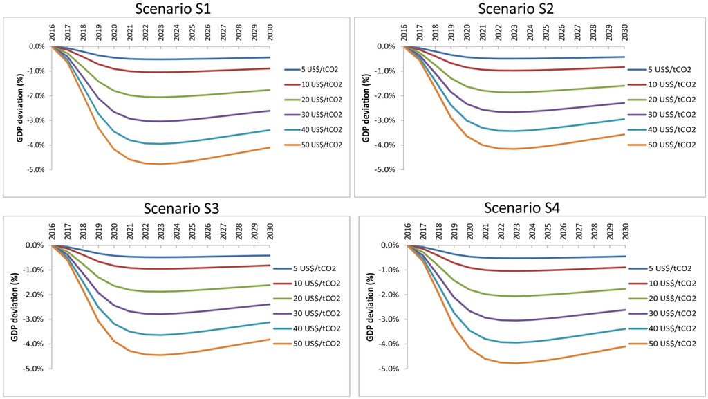
Figure 11.
Effect on the level of GDP (% over baseline deviations).
In all the cases a negative impact on GDP pathway is observed and it depends on the level of the tax. For example, for a carbon tax of 5 US$/tCO2e the maximum GDP reduction would be 0.4% by 2030. While for a carbon tax of 20 US$/tCO2e the maximum GDP reduction would be between 1.6% and 1.8% by 2030. Table 5 shows the equivalent average annual GDP growth rate observed after the carbon tax is applied (for the period 2017–2030). For example, in the case of a tax of 5 US$/tCO2e, the GDP growth rate would be between 3.47% versus 3.5% in the baseline scenario, and in the case of a tax of 20 US$/tCO2e, the GDP growth rate would be between 3.37% and 3.38% versus 3.5% in the baseline scenario.
Table 5.
Impact of carbon tax on the annual GDP growth rate.
| Carbon Tax (US$/tCO2e) | Scenario 1 | Scenario 2 | Scenario 3 | Scenario 4 | ||||
|---|---|---|---|---|---|---|---|---|
| GDP Growth Rate (%) | GDP Growth Rate Reduction (%) | GDP Growth Rate (%) | GDP Growth Rate Reduction (%) | GDP Growth Rate (%) | GDP Growth Rate Reduction (%) | GDP Growth Rate (%) | GDP Growth Rate Reduction (%) | |
| 5 | 3.47% | 0.03% | 3.47% | 0.03% | 3.47% | 0.03% | 3.47% | 0.03% |
| 10 | 3.43% | 0.07% | 3.44% | 0.06% | 3.44% | 0.06% | 3.43% | 0.07% |
| 20 | 3.37% | 0.13% | 3.38% | 0.12% | 3.38% | 0.12% | 3.37% | 0.13% |
| 30 | 3.30% | 0.20% | 3.33% | 0.17% | 3.32% | 0.18% | 3.30% | 0.20% |
| 40 | 3.25% | 0.25% | 3.28% | 0.22% | 3.27% | 0.23% | 3.25% | 0.25% |
| 50 | 3.19% | 0.31% | 3.23% | 0.27% | 3.21% | 0.29% | 3.19% | 0.31% |
It is important to note this analysis is not considering recycling of the results (tax collection is not reinvested in the economy), so the cases presented below can be considered as the worst case scenario (maximum negative effect) of this instrument over the GDP path. In addition, the emission reduction of these cases could be higher if the fiscal revenue of the carbon tax supports the implementation of mitigation actions or energy programs. However, in Chile these revenues are not necessary reallocated for these purposes. In fact, the revenues of the carbon tax will be used to funded part of the new tributary reform.
3.3. Comparison to Other Policies
The carbon tax is compared with other policies that stakeholders can apply in order to reduce GHG emissions: introduction of non-conventional renewable energy sources and a sectorial cap. Currently Chile has a non-conventional renewable energy (NCRE) law, based on a quota system, which states that the 20% of energy sales has to be provided by NCRE sources by 2025. This law was approved in 2013 (a previous version of this law, approved in 2008, stated that 10% of energy sales had to be provided by NCRE sources by 2024). We evaluated this potential increase up to 25% by 2030 (25/30 case) and 30% by 2030 (30/30 case). Table 6 shows the results of this evaluation.
The results show that a similar emission reduction can be obtained by increasing the NCRE quota, but the impact on the electricity price would be lower in comparison to the carbon tax scenarios. For example, for Scenario 1, the average annual emission reduction of the 25/30 case (1.0 million tCO2e) is similar to the emission reduction of 10 US$/tCO2e carbon tax case, and the emission reduction of the 30/30 case (1.9 million tCO2e) is similar to the emission reduction of 20 US$/tCO2e carbon tax case (1.8 million tCO2e).
Table 6.
Evaluation of a change to the current non-conventional renewable energy law.
| Unit Scenario | NCRE Case | ∆ OPEX | Carbon Tax Revenue | ∆ CAPEX | Cumulative ∆ Emission | Average ∆ Annual Emission | ∆ Electricity Price |
|---|---|---|---|---|---|---|---|
| MM US$ | MM US$ | MM US$ | MM tCO2e | MM tCO2e | US$/MWh | ||
| S1 | 25/30 | −124.9 | 0.0 | 202.1 | −13.9 | −1.0 | 0.1 |
| 30/30 | −334.4 | 0.0 | 516.6 | −27.2 | −1.9 | 0.3 | |
| S2 | 25/30 | −91.9 | 0.0 | 101.8 | −5.4 | −0.4 | 0.0 |
| 30/30 | −275.0 | 0.0 | 307.3 | −20.6 | −1.5 | 0.1 | |
| S3 | 25/30 | −289.8 | 0.0 | 381.8 | −13.2 | −0.9 | 0.2 |
| 30/30 | −349.3 | 0.0 | 570.7 | −34.8 | −2.5 | 0.4 | |
| S4 | 25/30 | −177.5 | 0.0 | 249.1 | −13.0 | −0.9 | 0.1 |
| 30/30 | −292.3 | 0.0 | 469.2 | −28.0 | −2.0 | 0.3 |
However, the electricity price increase is lower in both cases. In the first case the price of electricity would increase 0.1 US$/MWh versus 4.2 US$/MWh in the carbon tax case, and the second it would increase 0.3 US$/MWh versus 8.2 US$/MWh in the carbon tax case. Therefore, the impact on GDP will be lower. In this work the economic instruments to implement an increase of the NCRE quota are not analyzed. Currently, in Chile the introduction of renewable energy sources is financed by the private sector. The effect of NCRE law modifications over the path of gross domestic product (GDP) with respect to the baseline scenario is shown in the Figure 12.
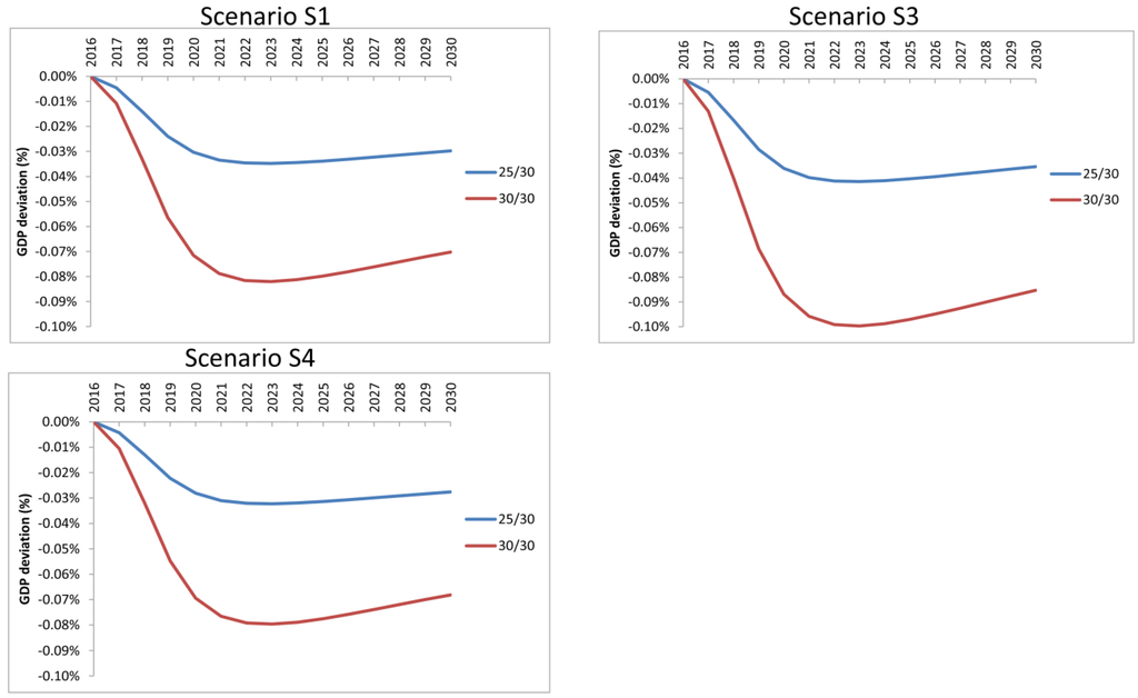
Figure 12.
Effect of NCRE law modifications on the level of GDP (% over baseline deviations).
In all the evaluated scenarios the GDP reduction is lower than 0.1% (Scenario S2 is not reported due to the low impact on the GDP). Additionally, a sectorial cap in the electricity generation sector is evaluated. The simulations were done considering an emission cap (maximum level of GHG emission) equals to the emission trajectory when the carbon tax is applied. The cap is introduced in the optimization problem as a constraint. The results of applying this cap are shown in Table 7.
Table 7.
Indicators associated to the application of sectorial cap on the Chilean electricity generation sector in the four scenarios (MM = million).
| Unit Scenario | Cap Scenario | ∆ OPEX | Carbon Tax Revenue | ∆ CAPEX | Cumulative ∆ Emission | Average ∆ Annual Emission | ∆ Electricity Price |
|---|---|---|---|---|---|---|---|
| MM US$ | MM US$ | MM US$ | MM tCO2e | MM tCO2e | US$/MWh | ||
| S1 | Cap5 | −58.7 | 0.0 | 62.4 | −1.2 | −0.1 | 0.0 |
| Cap10 | −149.3 | 0.0 | 189.2 | −13.6 | −1.0 | 0.1 | |
| Cap20 | −622.0 | 0.0 | 745.7 | −25.0 | −1.8 | 0.2 | |
| Cap30 | −932.2 | 0.0 | 1195.4 | −40.9 | −2.9 | 0.5 | |
| Cap40 | −1999.6 | 0.0 | 3279.2 | −139.8 | −10.0 | 2.3 | |
| Cap50 | −2926.9 | 0.0 | 4590.0 | −162.4 | −11.6 | 3.0 | |
| S2 | Cap5 | −459.2 | 0.0 | 488.0 | −21.2 | −1.5 | 0.1 |
| Cap10 | −857.4 | 0.0 | 955.9 | −48.6 | −3.5 | 0.2 | |
| Cap20 | −1916.3 | 0.0 | 2371.4 | −125.2 | −8.9 | 0.8 | |
| Cap30 | −3121.5 | 0.0 | 4057.0 | −170.9 | −12.2 | 1.7 | |
| Cap40 | −3708.9 | 0.0 | 5084.8 | −195.6 | −14.0 | 2.5 | |
| Cap50 | −3741.6 | 0.0 | 5140.5 | −197.0 | −14.1 | 2.5 | |
| S3 | Cap5 | −60.0 | 0.0 | 75.4 | −8.3 | −0.6 | 0.0 |
| Cap10 | −236.1 | 0.0 | 261.9 | −11.0 | −0.8 | 0.0 | |
| Cap20 | −499.4 | 0.0 | 594.8 | −22.5 | −1.6 | 0.2 | |
| Cap30 | −968.8 | 0.0 | 1201.2 | −36.0 | −2.6 | 0.4 | |
| Cap40 | −1516.3 | 0.0 | 2209.5 | −76.5 | −5.5 | 1.2 | |
| Cap50 | −2335.5 | 0.0 | 3470.8 | −104.4 | −7.5 | 2.0 | |
| S4 | Cap5 | −104.3 | 0.0 | 107.8 | −2.4 | −0.2 | 0.0 |
| Cap10 | −227.9 | 0.0 | 242.5 | −5.3 | −0.4 | 0.0 | |
| Cap20 | −457.0 | 0.0 | 533.9 | −15.7 | −1.1 | 0.1 | |
| Cap30 | −913.4 | 0.0 | 1286.7 | −46.4 | −3.3 | 0.7 | |
| Cap40 | −2160.3 | 0.0 | 3388.9 | −130.5 | −9.3 | 2.2 | |
| Cap50 | −2738.0 | 0.0 | 4325.9 | −152.6 | −10.9 | 2.8 |
- ◾
- Cap5: in this case the emission cap is equal to the emission trajectory that we got when the carbon tax of 5 US$/tCO2e is applied;
- ◾
- Cap10: in this case the emission cap is equal to the emission trajectory that we got when the carbon tax of 10 US$/tCO2e is applied;
- ◾
- Cap20: in this case the emission cap is equal to the emission trajectory that we got when the carbon tax of 20 US$/tCO2e is applied;
- ◾
- Cap30: in this case the emission cap is equal to the emission trajectory that we got when the carbon tax of 30 US$/tCO2e is applied;
- ◾
- Cap40: in this case the emission cap is equal to the emission trajectory that we got when the carbon tax of 40 US$/tCO2e is applied;
- ◾
- Cap50: in this case the emission cap is equal to the emission trajectory that we got when the carbon tax of 50 US$/tCO2e is applied.
Similar to the previous analysis, the results show that the same GHG emission reduction can be obtained by applying a cap in comparison to the carbon tax scenarios, however, the price of electricity would increase less than in the carbon tax cases. For example, in the Scenario 1, the Cap10 and Cap20 cases would increase the price of the electricity by 0.1 and 0.2 US$/MWh, respectively, versus 4.2 and 8.2 US$/MWh in the cases where the carbon tax is applied. The effect of the emission cap on the gross domestic product (GDP) path with respect to the baseline scenario is shown in the Figure 13. In all the scenarios the GDP reduction is lower than 1%, which is lower than the observed reductions in the carbon tax scenarios.
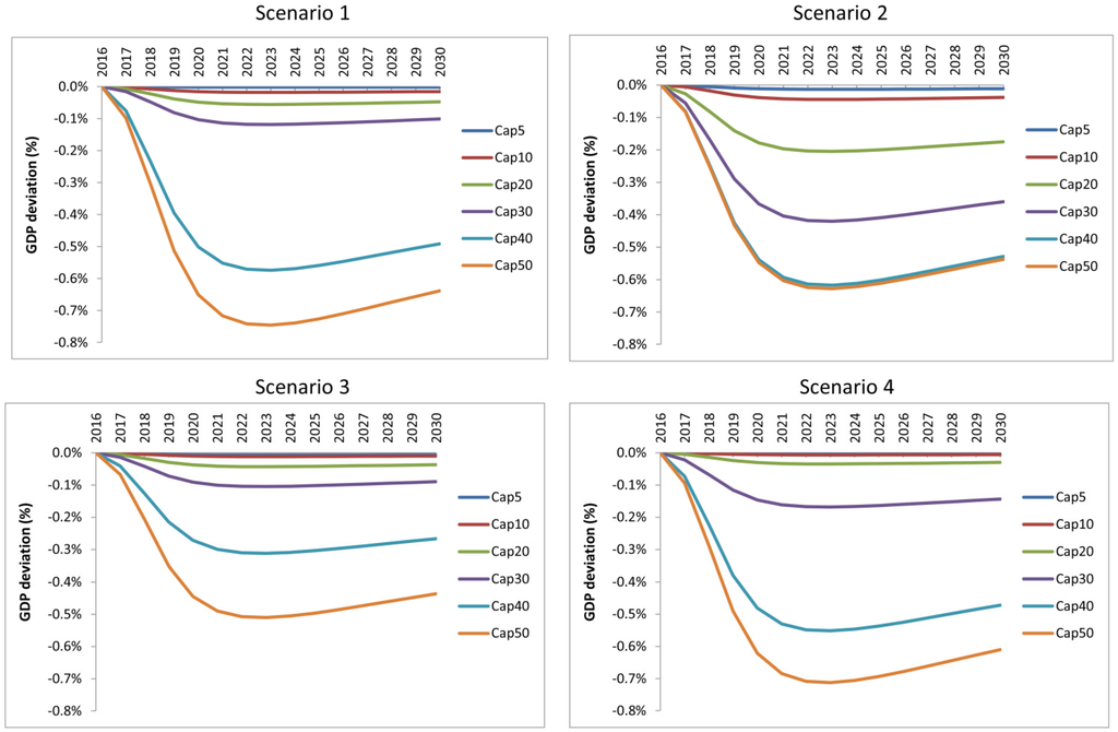
Figure 13.
Effect of sectoral cap on the level of GDP (% over baseline deviations).
4. Conclusions
The economy-wide implications of a carbon tax applied on the Chilean electricity market were successfully evaluated. A novel approach is proposed to integrate results from the electricity generation model and a macroeconomic DSGE model. The results show that the carbon tax has a negative impact on the GDP pathway, and the effectiveness of this policy, in the case of Chile, depends on some variables which are not controlled by policy makers such as non-conventional renewable energies investment cost projections, prices of LNG, and the exploitation of hydroelectric resources. Therefore, it is recommended that different development scenarios be evaluated in order to estimate the impact on GHG emission reduction of this policy. In a scenario with a carbon tax of 20 US$/tCO2e, the annual average emission reduction would be between 1.1 and 9.1 million tCO2e. However, the price of the electricity (electricity generation level) would increase between 8.3 and 9.6 US$/MWh, which is equivalent to a 7.4% and 8.5% with respect to the current price of electricity. This price shock decreases the annual GDP growth rate by a maximum value of 0.13%. It means that the average yearly GDP growth rate will be 3.37% versus 3.5% in the baseline scenario. On the other hand, alternative policies such as an increase to the quota of non-conventional renewable energy sources and a sectorial cap were evaluated. The results show that the same emission reductions can be achieved with these policies, but with a lower impact on the electricity price and the GDP pathway. Future work considers extending the proposed approach including the theoretical behavior of the iterative linkage between the two models (sectoral and DSGE) and the simulation of gradual tax rate penetration.
Acknowledgments
The paper was supported by Climate and Development Knowledge Network (CDKN), Mitigation Action Plans and Scenarios (MAPS) Programme and CONICYT/FONDAP/15110019.
Author Contributions
Carlos Benavides proposed the general methodology, developed the sectoral model to simulate the impact of the carbon tax on the electricity generation sector, and managed the paper project. Luis Gonzales contributed to develop the economic approach, designed the link between the sectoral and macroeconomic models, calibrated and performed the simulations on the DSGE model. Gonzalo Garcia contributed to develop the economic approach and gave technical support to do the simulation on the DSGE model. Rodrigo Fuentes supervised the results and methodology to evaluate the macroeconomic impacts of the carbon tax. Manuel Diaz helped with the overall coordination and result analysis. Rodrigo Palma supervised and contributed to the general methodology and analyzed the results. Catalina Ravizza helped to design the methodology. All the authors contributed to the state of the art, preparation, and approval of the manuscript.
Annex
Figure 14 shows the investment costs in the power generation sector that were considered for the preliminary calibration for the SIC and the SING.
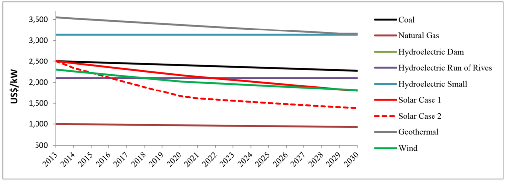
Figure 14.
Investment cost (US$/kW).
Figure 15 shows the LNG prices projection considered in this paper.
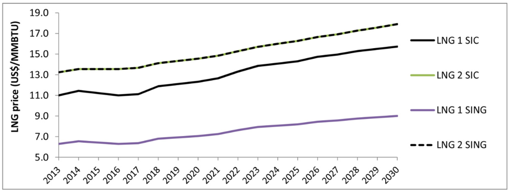
Figure 15.
LNG prices projection. LNG 1 SIC and LNG 1 SING are the prices of LNG for plants which have open access to the LNG terminal in SIC and SING, respectively. LNG 2 SIC and LNG 2 SING is the price for plant which have not open access to LNG terminal.
Conflicts of Interest
The authors declare no conflict of interest.
References
- Chile’s First Biennial Update Report to the United Nations Framework Convention on Climate Change; Ministry of Environment: Santiago, Chile, 2011.
- MAPS-Chile Project. Opciones de mitigación para enfrentar el cambio climático: resultados de Fase 2. Ministry of Environment: Santiago, Chile, 2014. Available online: http://mapschile.cl/files/Resultados_de_Fase_2_mapschile_2910.pdf (accessed on 4 January 2015). (In Spanish)
- SBS. Factbox: Carbon Taxes around the World. 2013. Available online: http://www.sbs.com.au/news/article/1492651/Factbox-Carbon-taxes-around-the-world (accessed on 4 January 2015).
- Capros, P.; Paroussos, L.; Fragkos, P.; Tsani, S.; Boitier, B.; Wagner, F.; Busch, S.; Resch, G.; Blesl, M.; Bollen, J. European decarbonisation pathways under alternative technological and policy choices: A multi-model analysis. Energy Strategy Rev. 2014, 2, 231–245. [Google Scholar] [CrossRef]
- Capros, P.; Paroussos, L.; Fragkos, P.; Tsani, S.; Boitier, B.; Wagner, F.; Busch, S.; Resch, G.; Blesl, M.; Bollen, J. Description of models and scenarios used to assess European decarbonisation pathways. Energy Strategy Rev. 2014, 2, 220–230. [Google Scholar] [CrossRef]
- European Commision (EC). Impact Assessment on Energy and Climate Policy up to 2030; European Commission (EC): Brussels, Belgium, 2014. [Google Scholar]
- Moyo, A.; Winker, H.; Wills, W. The Challenges of Linking Sectoral and Economy-Wide Models. MAPS-Programme. Available online: http://www.mapsprogramme.org/wp-content/uploads/Challenges-of-Linking_Brief.pdf (accessed on 5 January 2015).
- Vorster, S.; Winkler, H.; Jooste, M. Mitigating climate change through carbon pricing: An emerging policy debate in South Africa. Clim. Dev. 2011, 3, 242–258. [Google Scholar] [CrossRef]
- Winkler, H. Taking Action on Climate Change: Long-term Mitigation Scenarios for South Africa; UCT Press: Cape Town, South Africa, 2010. [Google Scholar]
- Alton, T.; Arndt, C.; Davies, R.; Hartley, F.; Makrelov, K.; Thurlow, J.; Ubogu, D. Introducing carbon taxes in South Africa. Appl. Energy 2014, 116, 344–354. [Google Scholar] [CrossRef]
- Thepkhun, P.; Limmeechokchai, B.; Fujimori, S.; Masui, T.; Shrestha, R. Thailand’s Low-Carbon Scenario 2050: The AIM/CGE analyses of CO2 mitigation measures. Energy Policy 2013, 62, 561–572. [Google Scholar] [CrossRef]
- Chi, Y.; Guo, Z.; Zheng, Y.; Zhang, X. Scenarios analysis of the energies’ consumption and carbon emissions in China based on a dynamic CGE model. Sustainability 2014, 6, 487–512. [Google Scholar] [CrossRef]
- Guo, Z.; Zhang, X.; Zheng, Y.; Rao, R. Exploring the impacts of a carbon tax on the Chinese economy using a CGE model with a detailed disaggregation of energy sectors. Energy Econ. 2014, 45, 455–462. [Google Scholar] [CrossRef]
- Böhringer, C.; Rutherford, T. Transition towards a low carbon economy: A computable general equilibrium analysis for Poland. Energy Policy 2013, 55, 16–26. [Google Scholar] [CrossRef]
- Mahmood, A.; Marpaung, C. Carbon pricing and energy efficiency improvement—Why to miss the interaction for developing economies? An illustrative CGE based application to the Pakistan case. Energy Policy 2014, 67, 87–103. [Google Scholar]
- Bukowski, M.; Kowal, P. Large Scale, Multi-sector DSGE Model as a Climate Policy Assessment Tool—Macroeconomic Mitigation Options (MEMO) Model for Poland; IBS Working Paper; Institute for Structural Research (IBS): Warsaw, Poland, 2010. [Google Scholar]
- Mongelli, I.; Tassielli, G.; Notarnicola, B. Carbon Tax and its Short-Term Effects in Italy: An evaluation through the Input-Output model. In Handbook of Input-Output Economics in Industrial Ecology; Springer: Dordrecht, The Netherlands, 2009. [Google Scholar]
- Syri, S.; Lehtilä, A.; Ekholm, T.; Savolainen, I.; Holttinen, H.; Peltola, E. Global energy and emissions scenarios for effective climate change mitigation—Deterministic and stochastic scenarios with the TIAM model. Int. J. Greenh. Gas Control 2008, 2, 274–285. [Google Scholar]
- Anandarajah, G.; Gambhir, A. India’s CO2 emission pathways to 2050: What role can renewables play? Appl. Energy 2014, 131, 79–86. [Google Scholar] [CrossRef]
- Fairuz, S.M.C.; Sulaiman, M.Y.; Lim, C.H.; Mat, S.; Ali, B.; Saadatian, O.; Ruslan, M.H.; Salleh, E.; Sopian, K. Long term strategy for electricity generation in Peninsular Malaysia—Analysis of cost and carbon footprint using MESSAGE. Energy Policy 2013, 62, 493–502. [Google Scholar] [CrossRef]
- Matsuoka, Y.; Kainuma, M.; Morita, T. Scenario analysis of global warming using the Asian Pacific Integrated Model (AIM). Energy Policy 1995, 23, 357–371. [Google Scholar] [CrossRef]
- Zang, H.; Xu, Y.; Li, W. An uncertain energy planning model under carbon taxes. Front. Environ. Sci. Eng. 2012, 6, 549–558. [Google Scholar] [CrossRef]
- Kainuma, M.; Matsuoka, Y.; Morita, T.; Hibino, G. Development of an end-use model for analyzing policy options to reduce greenhouse gas emissions. IEEE Trans. Syst. Man Cybern. C Appl. Rev. 1999, 29, 317–324. [Google Scholar] [CrossRef]
- Careri, F.; Genesi, C.; Marannino, P.; Montagna, M. Generation expansion planning in the age of green economy. IEEE Trans. Power Syst. 2011, 26, 2214–2223. [Google Scholar] [CrossRef]
- Chen, Q.; Kang, C.; Xia, Q.; Zhong, J. Power generation expansion planning model towards low-carbon economy and its application in China. IEEE Trans. Power Syst. 2010, 25, 1117–1125. [Google Scholar] [CrossRef]
- Wei, W.; Liang, Y.; Liu, F.; Mei, S.; Tian, F. Taxing strategies for carbon emissions: A bilevel optimization approach. Energies 2014, 7, 2228–2245. [Google Scholar] [CrossRef]
- National Technical University of Athens. The GEM-E3 Model Reference Manual. Available online: http://www.e3mlab.ntua.gr/manuals/GEMref.PDF (accessed on 5 March 2015).
- Rodrigues, R.; Linares, P. Electricity load level detail in computational general equilibrium—Part I—Data and calibration. Energy Econ. 2014, 46, 258–266. [Google Scholar] [CrossRef]
- Del Negro, M.; Schorfheide, F. DSGE Model-Based Forecasting. Elliott, G., Timmermann, A., Eds.; In Handbook of Economic Forecasting SET 2A-2B; Elsevier: Amsterdam, The Netherlands, 2013; Volume 2, pp. 57–140. [Google Scholar]
- Edge, R.; Gurkaynak, R. How Useful are Estimated DSGE Model Forecasts? Available online: http://www.federalreserve.gov/pubs/feds/2011/201111/ (accessed on 7 January 2015).
- Energy Ministry, GIZ. Renewable Energy in Chile, wind, solar and hydroelectric potential in Chile. 2014. Available online: http://www.minenergia.cl/archivos_bajar/Estudios/Potencial_ER_en_Chile_AC.pdf (accessed on 4 January 2015). (In Spanish)
- Mercure, J.F.; Pollitt, H.; Chepreecha, U.; Salas, P.; Foley, A.M.; Holden, P.B.; Edwards, N.R. The dynamics of technology diffusion and the impacts of climate policy instruments in the decarbonisation of the global electricity sector. Energy Policy 2014, 73, 686–700. [Google Scholar] [CrossRef]
- Chile 2030 Energy Scenario Platform. Santiago, Chile, 2014. Available online: http://escenariosenergeticos.cl/wp-content/uploads/Escenarios_Energeticos_2013.pdf (accessed on 7 January 2015). (In Spanish)
- CDEC-SIC (Central Interconnected System Load Economic Dispatch Center). Available online: http://www.cdecsic.cl/ (accessed on 6 January 2015). (In Spanish)
- CDEC-SING (Center for Economic Load Dispatch of Northern Interconnected System). Available online: http://cdec2.cdec-sing.cl/ (accessed on 6 January 2015). (In Spanish)
- National Energy Comission. April 2014 Node Price Report of the Central Interconnected System. Santiago, Chile, 2014. Available online: http://www.cne.cl/tarificacion/electricidad/precios-de-nudo-de-corto-plazo/abril-2014 (accessed on 6 January 2014). (In Spanish)
- National Energy Comission. April 2014 Node Price Report of Norte Grande Interconnected System. Santiago, Chile, 2014. Available online: http://www.cne.cl/tarificacion/electricidad/precios-de-nudo-de-corto-plazo/abril-2014 (accessed on 6 January 2014). (In Spanish)
- Medina, J.; Soto, C. Model for Analysis and Simulations: A Small Open Economy DSGE for Chile. Central Bank of Chile, 2006. Available online: http://www.bcentral.cl/conferencias-seminarios/otras-conferencias/pdf/modelling2006/soto_medina.pdf (accessed on 7 January 2015).
- Medina, J.P.; Soto, C. The Chilean Business Cycle through the lens of Stochastic General Equilibrium Model. Working Papers 457. Central Bank of Chile, 2007. Available online: http://www.bcentral.cl/conferencias-seminarios/otras-conferencias/pdf/variables/Medina_Soto.pdf (accessed on 7 January 2015).
- Calvo, G. Staggered prices in utility-maximizing framework. J. Monet. Econ. 1983, 12, 383–398. [Google Scholar] [CrossRef]
- Christiano, L.; Eichenbaum, M.; Evans, C. Nominal rigidities and the dynamic effects of a shock to monetary policy. J. Political Econ. 2005, 113, 1–45. [Google Scholar] [CrossRef]
- Erceg, C.; Henderson, D.W.; Levin, A.T. Optimal monetary policy with staggered wage and price contracts. J. Monet. Econ. 2000, 46, 281–313. [Google Scholar] [CrossRef]
- GLPK. Available online: https://www.gnu.org/software/glpk/ (accessed on 7 January 2015).
- CPLEX Optimizer. Available online: http://www-01.ibm.com/software/commerce/optimization/cplex-optimizer/ (accessed on 7 January 2015).
- Cerda, R. Implementation of DSGE Model in MATHLAB; Institute of Economics, Pontifical Catholic University of Chile: Santiago, Chile, 2010. [Google Scholar]
© 2015 by the authors; licensee MDPI, Basel, Switzerland. This article is an open access article distributed under the terms and conditions of the Creative Commons Attribution license (http://creativecommons.org/licenses/by/4.0/).