1. Introduction
Most of the energy produced by internal combustion engines is expelled to the environment via the exhaust and coolant systems. The expelled energy makes the engine running cost high and is one of the major causes of global warming and environmental pollution. In order to reduce fuel consumption, waste heat recovery (WHR) has been a growth research area in recent years. The WHR system is used to collect the heat from the exhaust or coolant and convert it into either mechanical or electrical power, which increases the thermal efficiency of the engine [
1]. Among different methods to recover the waste heat, the Organic Rankine Cycle (ORC) is the most promising and widely used technology because of simplicity and availability of its components [
2,
3]. The working fluid used in the ORC is an organic substance (
i.e., hydrocarbons or refrigerants), which has the properties of high molecular weight and low boiling point that are suitable for low grade heat recovery applications.
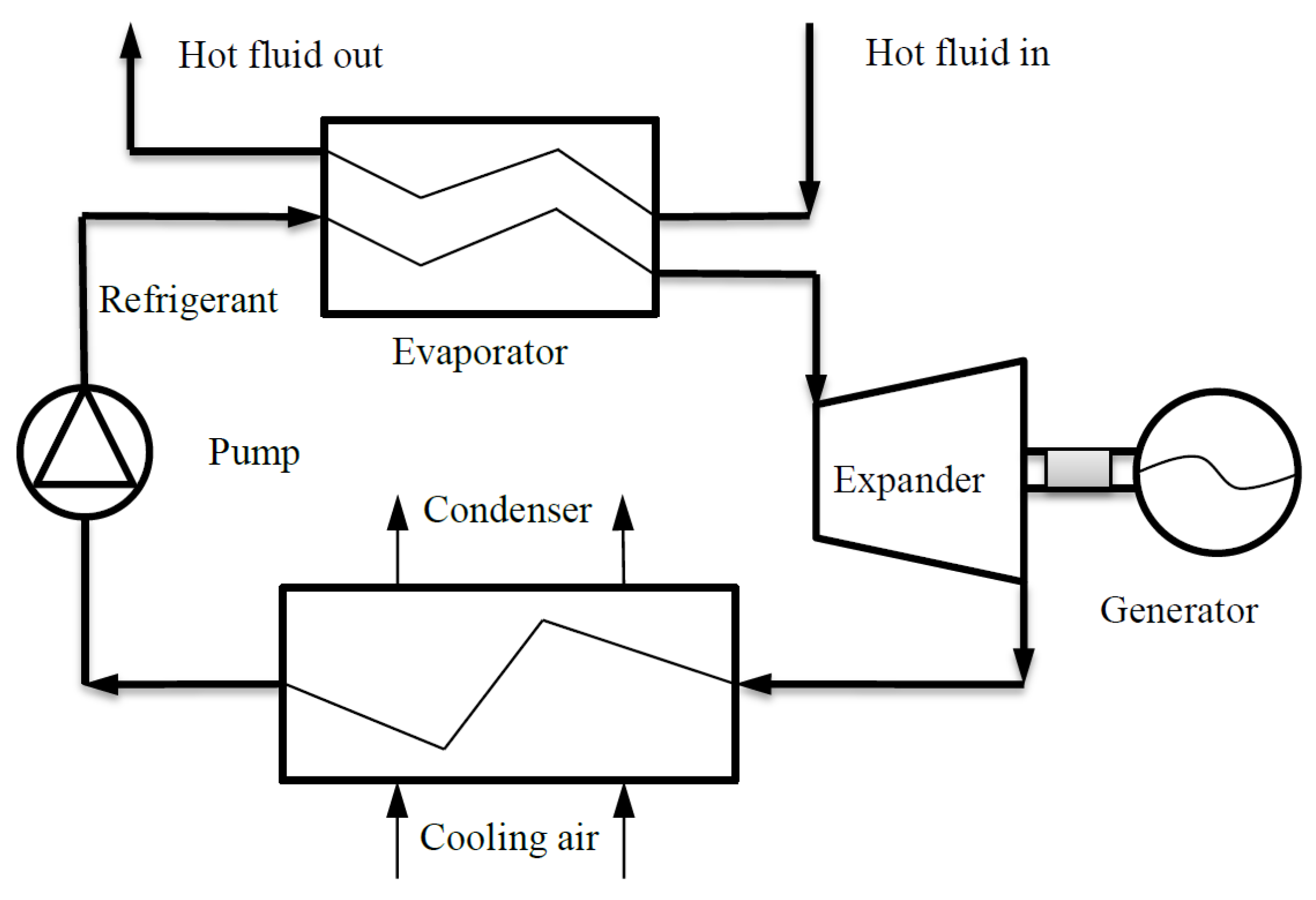
The ORC WHR system consists of four major components: pump, evaporator, expander and condenser, as shown in
Figure 1. Liquid refrigerant is pumped to the evaporator where it is heated and vaporized by the heat sources. This vaporized fluid is then expanded and produces mechanical energy output through the shaft of the expander. A generator is normally coupled with the expander shaft to convert mechanical energy into electrical power. Exhaust products from the expander pass through the condenser where secondary cooling fluid removes extra heat and converts the exhaust back to a liquid.
Figure 1.
Components of a typical Organic Rankine Cycle (ORC) WHR system.
Figure 1.
Components of a typical Organic Rankine Cycle (ORC) WHR system.
Depending on the working pressure, the evaporator of the ORC WHR can operate under two conditions: Subcritical and supercritical. The operating pressure of the subcritical evaporator is below the critical pressure of the working fluid, whereas in supercritical conditions, it is above the critical pressure. The operating pressure of the evaporator has an effective influence on the work output and efficiency of the ORC based WHR system. The efficiency of an ORC in subcritical conditions is low as the cycle is run at a lower pressure ratio and the exergy destruction and loss is found to be high [
4]. The initial investigation carried out by Glover
et al. [
1], Schuster
et al. [
4], Shu
et al. [
5] and Gao
et al. [
6] show that the heat addition to the working fluid at supercritical pressure can lead to the highest efficiency of the cycle. This is due to the higher net power output, lower exergy losses and destruction, and better thermal match between heat source and working fluid. However, the benefits of the supercritical ORC are dependent on the types of heat, working fluids, operating conditions and cycle configuration used. Lecompt
et al. [
7] showed that the second law efficiency of a supercritical cycle for low temperature waste heat recovery is 10.8% more than a subcritical cycle. Chen
et al. [
8] showed that a supercritical ORC with a zeotropic mixture as the working fluid can improve the thermal efficiency by 10%–30% more than the subcritical ORC.
Modelling of the evaporator in the ORC WHR system has been addressed in several reports [
2,
9,
10,
11,
12,
13,
14,
15,
16,
17]. Three common modelling techniques are normally used for the evaporator: single segment lump method, three zone method and distributed or finite volume (FV) method [
11]. The single segment technique treats the evaporator as a single-phase (
i.e., liquid) heat exchanger. This method is only appropriate when the specific heat capacity of the fluid does not change with temperature. A zone modelling technique can be used where the evaporator has three distinct phases: liquid, liquid-vapour and vapour zone [
15]. This method cannot be used where a distinct fluid phase is absent. The finite volume technique splits the evaporator into small segments and heat transfer equations are solved iteratively [
2,
18,
19]. In the FV method, the thermo-physical properties are assumed to be constants at each segment of the evaporator since the temperature variation of the segment is low and is normally neglected.
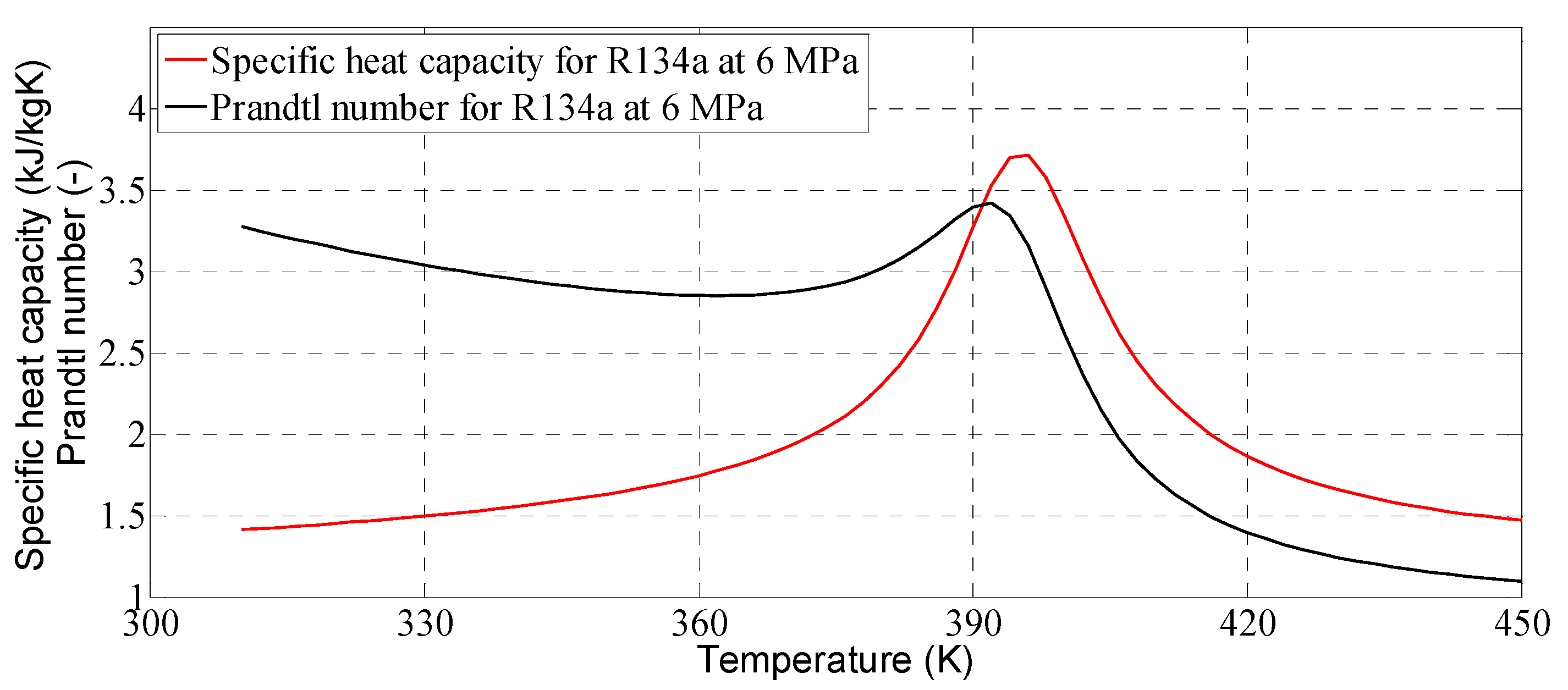
Although the calculations of the evaporator model using single segment or zone-wise methods are clear, the influence of the working pressure on the WHR system are not considered in these methods. When the evaporator operates under supercritical conditions, the thermo-physical properties of the working fluid change with temperature (
Figure 2) and there is no distinct fluids phase at these conditions [
18]. For these reasons, a single segment lump method with constant fluid properties or a zone-wise technique cannot be used to calculate the heat transfer under supercritical conditions. In order to capture the thermo-physical property changes of the fluid, the finite volume method [
18] has been developed for modelling of the evaporator in supercritical conditions.
Figure 2.
Variation of specific heat capacity and Prandtl number with temperature.
Figure 2.
Variation of specific heat capacity and Prandtl number with temperature.
Despite high accuracy and robustness [
18], the finite volume modelling technique is a highly time consuming method since it consists of many iterative loops [
11,
19], therefore, it has a limitation in real time control applications. In order to reduce the computation time of the evaporator model, a new evaporator model using the fuzzy inference technique is introduced and described in this paper.
Fuzzy logic [
20] has been used to identify nonlinear systems, which avoids the need to have a complex model and saves computation cost and time during simulation and real time control applications [
21]. A fuzzy model is generally built with experimental input-output data or an original mathematical model of the system [
22]. Both the antecedent (input) and the consequent (output) of the fuzzy model are represented by fuzzy sets [
23]. A defuzzification unit converts the fuzzy output into a single value (crisp value) by combining and weighting of the fuzzy sets. In order to assess fuzzy model performance, the crisp outputs can be compared with the actual values of the system [
23].
This paper investigates two different modelling techniques for the evaporator operating at the supercritical condition. The first model uses the finite volume method; while the second model uses the fuzzy inference technique. Details of the fuzzy based evaporator model and its performance compared with the conventional finite volume method is presented in this paper.
The rest of the paper is presented as follows:
Section 2 introduces different types of evaporator used in WHR systems. A detailed description and the working principles of the finite volume along with its simulation results are presented in
Section 3. The design of the fuzzy based evaporator model and a comprehensive analysis of its outputs and the accuracy in comparison with the finite volume model are presented in
Section 4. Concluding remarks are provided in
Section 5.
3. Modelling of Evaporator Using the Finite Volume Method
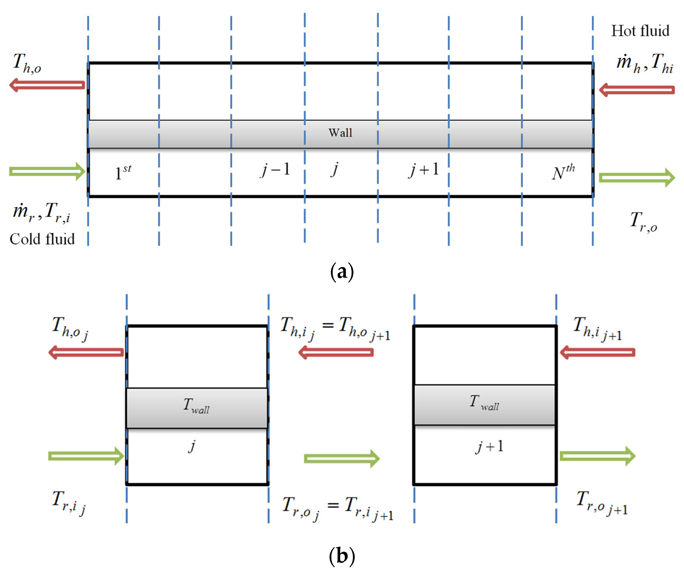
In the finite volume (FV) technique, the evaporator is divided into small segments along the flow direction as shown in
Figure 4, and the heat transfer equations for each segment are solved iteratively [
19]. The FV evaporator model is built with the following fundamental assumptions:
There is no pressure loss in either the hot or cold side of the heat exchanger.
Heat transfer from or to the surrounding environment is negligible.
Heat exchanger fouling is not included in the model.
Heat from the hot fluid is completely transferred to the working fluid.
Figure 4.
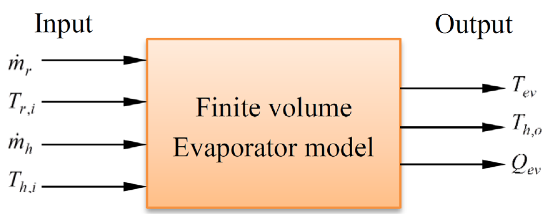
(a) Finite volume evaporator model; (b) Relationship between input and output variables.
Figure 4.
(a) Finite volume evaporator model; (b) Relationship between input and output variables.
The input parameters of the evaporator model are: mass flow rate and temperature of the refrigerant (
) and hot fluid (
) and the outputs parameters are: evaporator power (
) and outlet temperature (
or
and
), as shown in
Figure 5. Among the input parameters, the refrigerant inlet temperature is assumed to be constant and equal to a temperature of 303 K. However, using FV method, the outlet temperatures of the hot and cold fluid are not known, but are initially estimated and an iteration process is carried out for each segment. The iteration starts from the
segment and finishes at the
segment as shown in
Figure 4. For each segment or cell
in
Figure 4, the heat transfer from the hot fluid to the wall and the wall to the refrigerant can be calculated in (1) and (2) as follows:
Figure 5.
Input-output of finite volume evaporator model.
Figure 5.
Input-output of finite volume evaporator model.
where
and
refers to the amount of heat (kW) transferred from the hot fluid to the wall and the wall to the refrigerant respectively.
and
are the convective heat transfer coefficients (kW/m
2K) of the hot fluid and refrigerant with the wall.
and
are the heat transfer surface areas,
and
are the hot fluid and refrigerant’s average temperature, within each finite volume, respectively.
is the wall temperature, which can be obtained from the average of the hot fluid and refrigerant temperature of the cell. These parameters are calculated as follows:
where
,
are the hot fluid temperature and
,
are the refrigerant temperature at the inlet and outlet of each segment.
Heat transfer due to the change in temperature of the hot fluid is calculated in Equation (6); whereas heat transfer due to the change in enthalpy of the refrigerant is calculated in Equation (7) as follows:
where
(kg/s) and
(kg/s) are the mass flow rates of the hot fluid and refrigerant respectively,
(kJ/kg K) is the specific heat capacity of the hot fluid, and
(kJ/kg) is the enthalpy of the refrigerant.
The thermo-physical properties of the working fluid around the critical temperature are strongly variable at critical pressure [
18]. For this reason, the Jackson correlation for supercritical fluids [
28,
29] is used to calculate the Nusselt number
for the refrigerant in Equation (8). This neutralizes the variation effects around the pseudo-critical point. For the hot fluid, it is calculated with Equation (11) using the Dittus Boelter correlation as suggested by Sharabi
et al. [
30].
where
is the bulk temperature of the refrigerant,
is the pseudo-critical temperature of the refrigerant;
is the average specific heat capacity of the medium;
is the density of the working fluid at wall temperature and
is the density of the working fluid at bulk temperature;
and
are the enthalpy of the working fluid at wall and bulk temperature, respectively. In this case, the bulk temperature is the same as the average refrigerant temperature of the cell.
The convective heat transfer coefficients of the fluids are calculated in Equation (12) and the Reynolds number
is calculated in Equation (13):
where
is the hydraulic diameter of the plate heat exchanger,
is the density (kg/m
3) of the fluid,
is the viscosity (Pa.s) and
is the velocity of the fluids (m/s).
Figure 6 and
Figure 7 show the finite volume iteration process to calculate the outputs of the evaporator model. The steps of the iteration process are described as follows:
- Step 1:
All inputs of the model are defined at the beginning of the iteration process. The first segment is then initialized by assigning an initial inlet refrigerant temperature and assuming an initial hot fluid outlet temperature as shown in
Figure 6.
- Step 2:
Set the initial values for the inlet, outlet and wall temperatures of the segment
as shown in
Figure 7.
- Step 3:
When all inlet and outlet temperatures of the first segment are known, the wall temperature of the evaporator is iteratively evaluated until the heat transfer rates in Equations (1) and (2) are equal with a selected maximum deviation of .
- Step 4:
The heat transfer rate of the fluids at Step 3 is used to calculate the output variables of each segment by using the energy balance condition of the fluids. The iteration at this step is repeated until the deviations are within the allowable limits of the convergence values as shown in
Table 2. The values are a compromise chosen to reduce the computation time while achieving reasonable model accuracy.
- Step 5:
At this stage, the outlet variables of the first segment are all known. The iteration process continues along the refrigerant flow direction, the output variables of the first segment are used as the input of the second segment as shown in the
Figure 4b and the steps 2–4 repeated until the deviations are satisfied. This process is repeated until the
segment as shown in
Figure 6.
Figure 6.
Finite volume calculations for all segments of the evaporator.
Figure 6.
Finite volume calculations for all segments of the evaporator.
Figure 7.
Finite volume calculations for the first segment .
Figure 7.
Finite volume calculations for the first segment .
Table 2.
Convergence value for iteration loops.
Table 2.
Convergence value for iteration loops.
| Convergence Name | Convergence Value |
|---|
| ε1 | 0.1 |
| ε2 | 0.1 |
| ε3 | 0.1 |
| ε4 | 0.2 |
- Step 6:
At the end of the
segment, the calculated hot fluid temperature at the inlet of the evaporator
is obtained. This calculated temperature is then compared with the real hot fluid data. If the error between the calculated and real temperature is less than the deviation shown in
Table 2, the iteration process stops. Otherwise, the iteration process is repeated at steps 1–6.
Simulation Results of Finite Volume Evaporator Model
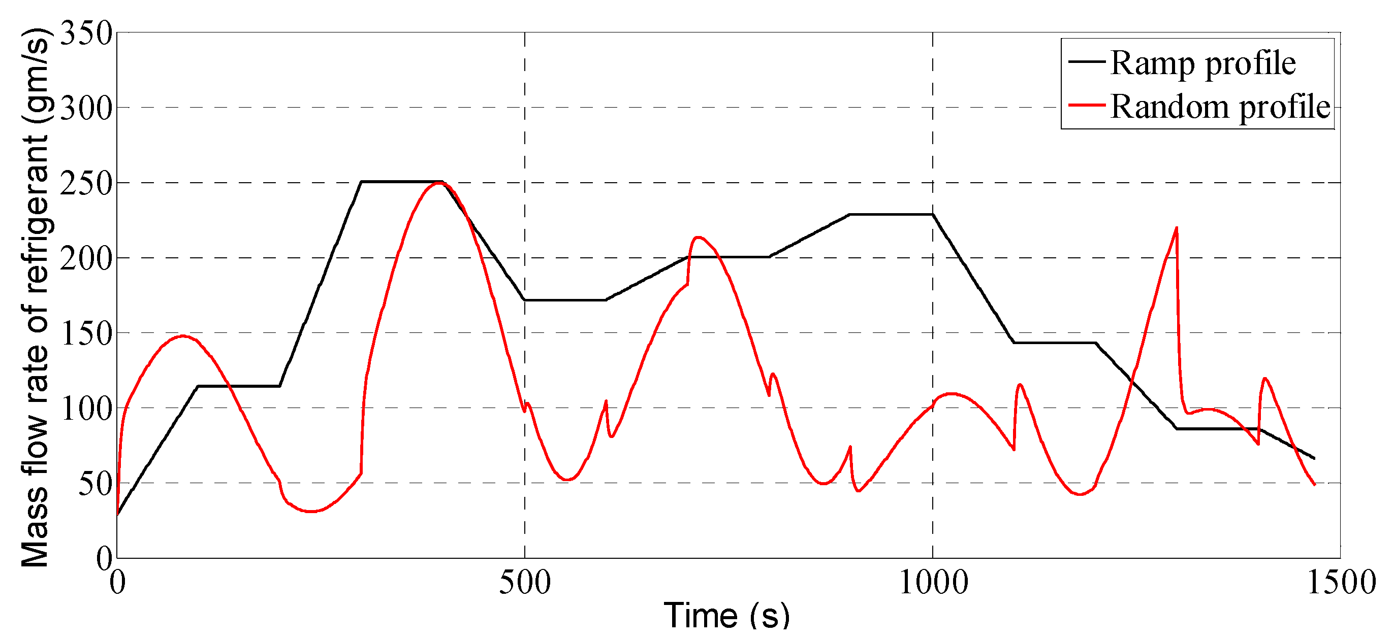
The working fluid used in the simulation of the evaporator is R134a refrigerant and hot water is used as the heat source. Several mass flow rate profiles of the R134a refrigerant were used to evaluate the evaporator model.
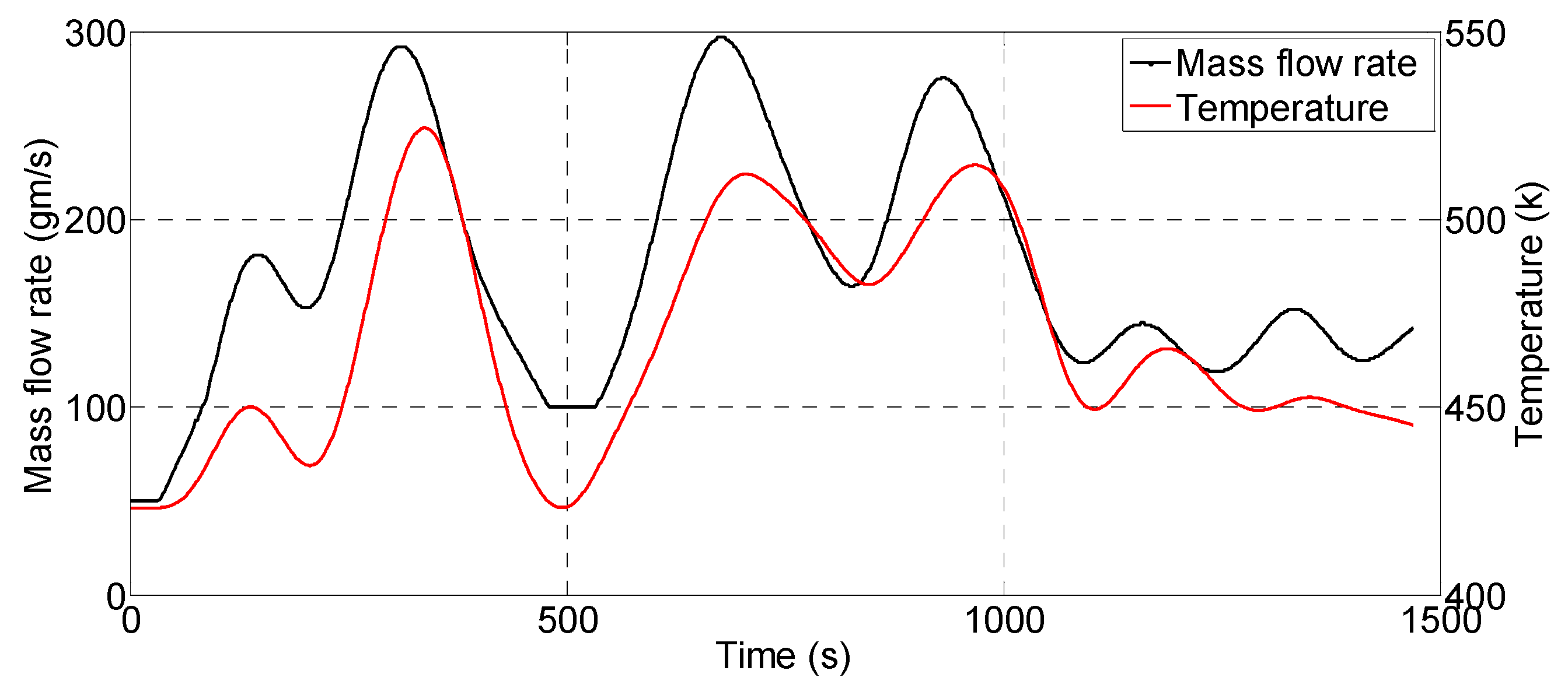
Figure 8 shows two different random mass flow rate profiles including a random ramp profile in the simulation. The range of these profiles was from 28.6 gm/s to 250 gm/s. These values were chosen based on the minimum and maximum delivery capacity of the pump normally used in the WHR process. The generic heat source in terms of variable mass flow rate and temperature (
Figure 9) defined by Quoilin
et al. [
2] was used in this paper. This heat source was considered to be the hot water under pressure and could typically represent the total heat that is collected from an internal combustion engine’s exhaust and coolant, via a secondery heat transfer fluid loop.
Figure 8.
The mass flow rate of refrigerant profiles.
Figure 8.
The mass flow rate of refrigerant profiles.
Figure 9.
Heat source mass flow rate and temperature.
Figure 9.
Heat source mass flow rate and temperature.
The performances of the evaporator model were tested at a supercritical pressure of 6 MPa. This value is far away from the critical pressure of the R134a refrigerant which is 4.06 MPa. As mentioned in Karellas
et al. [
18], when the pressure of the evaporator rises, the error of the finite volume calculation is reduced and the procedure converges with fewer segments. The numbers of segments for the evaporator were set to 20 in the simulation, as it is a good compromise between iteration time and the accuracy of the model. The pseudo-critical temperature of R134a was set to 395 K which is constant at the reference pressure of 6 MPa. The thermo-physical properties of the refrigerant and hot water used in the simulation were obtained from the U.S. National Institute of Standards and Technology (NIST) database called REFPROP [
31].
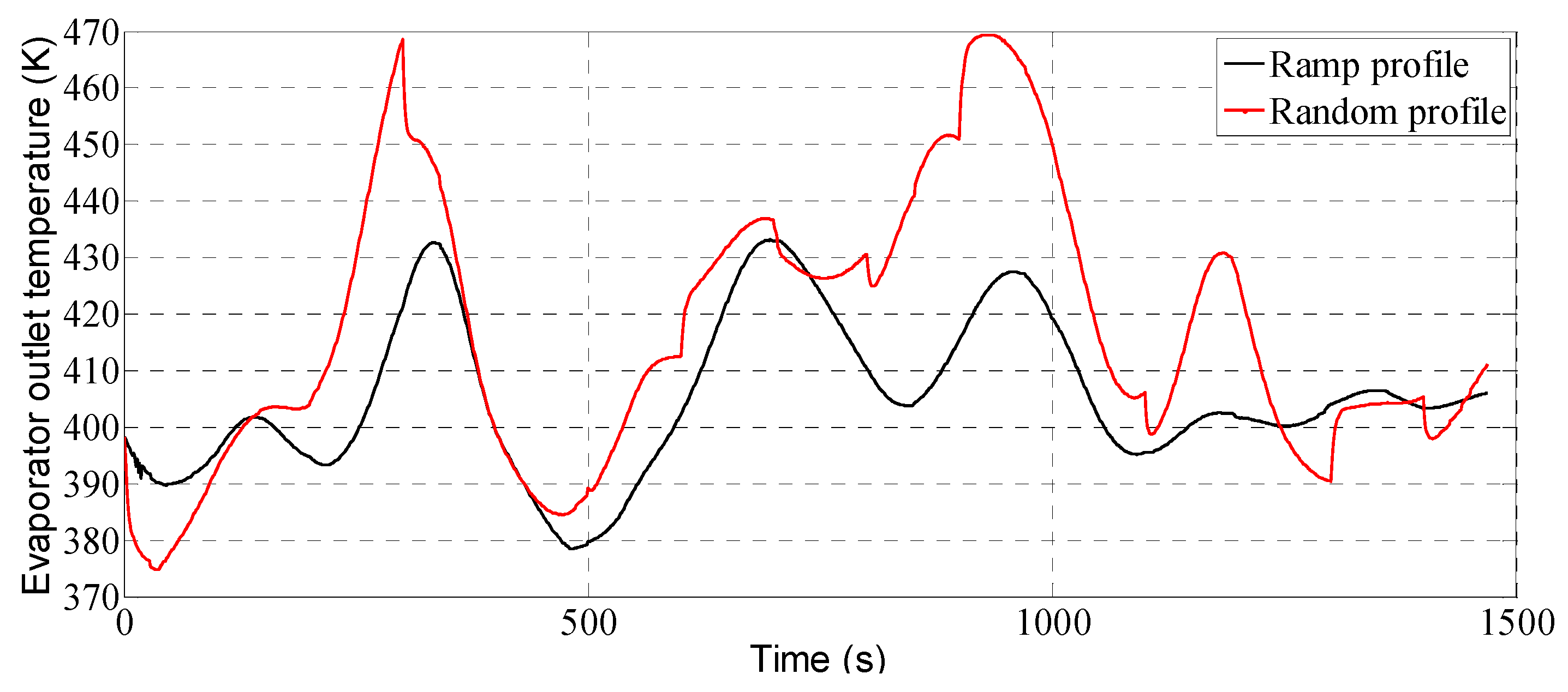
The evaporator power and evaporator outlet temperature from the FV model are shown in
Figure 10 and
Figure 11, respectively.
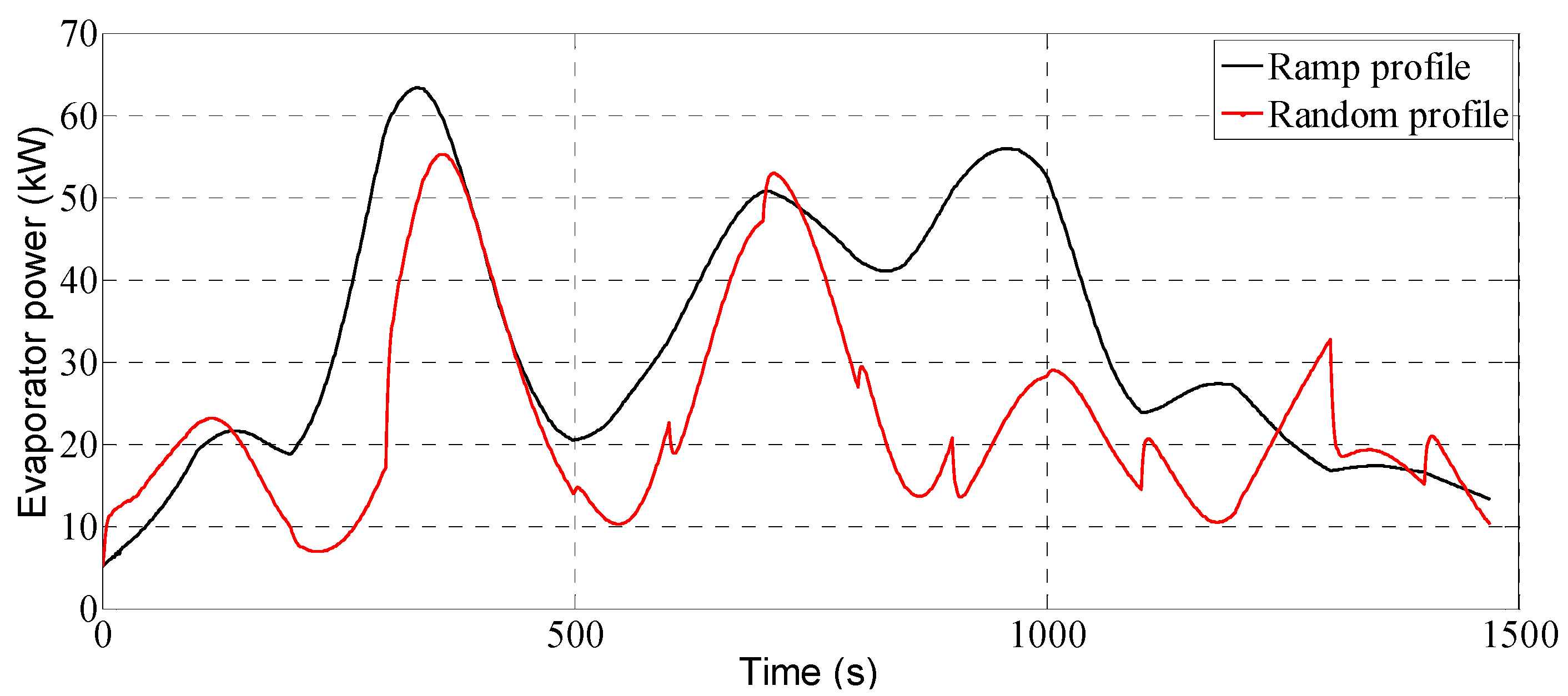
Figure 10 shows the variation of heat power absorbed by the evaporator with respect to the selected mass flow rate profiles in
Figure 8. It can be seen from the figure that a maximum heat of 63.3 kW for the ramp profile and 55.2 kW for the random profile can be recovered from the given heat sources. The variation of evaporator outlet temperature in
Figure 11 shows that a maximum temperature of 433 K for the ramp profile and 469 K for the random profile are achieved at the outlet of the evaporator.
Figure 10.
Evaporator power of the FV model.
Figure 10.
Evaporator power of the FV model.
Figure 11.
Evaporator outlet temperature of the FV model.
Figure 11.
Evaporator outlet temperature of the FV model.
The FV model was run on a personal computer, with the specification shown in
Table 3.
Table 4 shows the computation time of the finite volume model for the two different profiles. From the results, it can be observed that the computation time of the finite volume method is very high due to the many iterative loops used in the model.
Table 3.
Computer specifications.
Table 3.
Computer specifications.
| Operating System | Windows® 7 Enterprise 64-bits |
|---|
| Processor | Intel® Core™ i7-3770 CPU @3.40GHz; 16384MB RAM |
| Programming software | MATLAB® R2014a 64 bits |
Table 4.
Simulation time of the finite volume-based evaporator model.
Table 4.
Simulation time of the finite volume-based evaporator model.
| Input Profile (each profile contains 1470 data sets) | Simulation Time |
|---|
| Ramp profile | 13870 (s) |
| Random profile | 14826 (s) |
4. Fuzzy Evaporator Model
As described in the above section, although the calculation procedure of the evaporator model using the FV method is clear, the computation time is too high. This poor performance will restrict the model for use in a real time control systems. To overcome this drawback, a new fuzzy-based evaporator model is introduced. Detailed construction and working principle of the proposed fuzzy based evaporator model is described in this section.
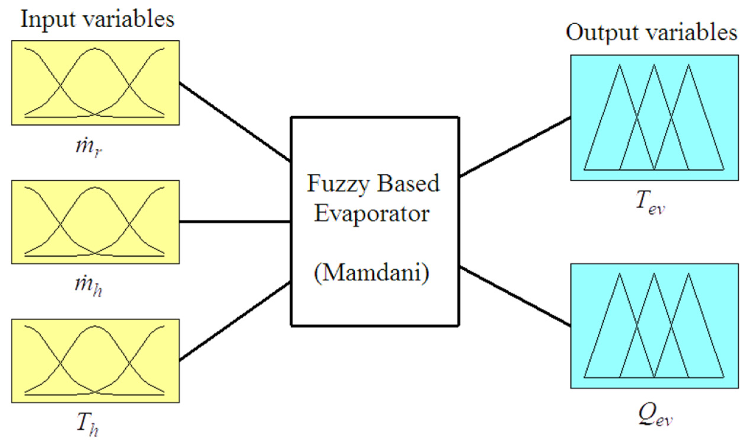
The fuzzy based evaporator model is designed with three inputs and two outputs and is shown in
Figure 12. The inputs of the model are mass flow rate of refrigerant
, mass flow rate of hot fluid
and temperature of hot fluid
; and the outputs are the evaporator power
and outlet temperature
.
Figure 12.
Three inputs and two outputs fuzzy inference system for the evaporator.
Figure 12.
Three inputs and two outputs fuzzy inference system for the evaporator.
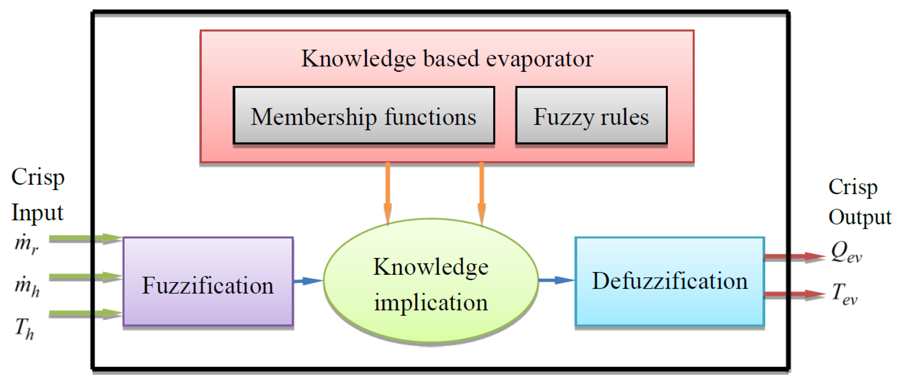
Figure 13 shows the structure of the fuzzy based evaporator model with three inputs and two outputs. The fuzzy evaporator model in this paper is built using the fuzzy technique introduced by Mamdani and Assilian [
20]. The fuzzy model represents the nonlinear system of the evaporator by mapping its input variables to the output variables. A fuzzy model typically consists of fuzzy logic, membership functions, fuzzy sets, and fuzzy rules [
22]. The fuzzy logic is a multivalued logical system that provides the value of an unknown output by attaching the degree of known input and output of the system [
32]. The inputs and outputs ranges of the evaporator model are divided into linguistic levels; each of these levels is called a membership function. The collection of membership functions is termed as a fuzzy set. The fuzzy rules of the evaporator are created using fuzzy IF-THEN statements. The fuzzy based evaporator model consists of a fuzzification unit, a knowledge based unit, an implication unit and a defuzzification unit as shown in
Figure 13.
Figure 13.
Fuzzy based evaporator model.
Figure 13.
Fuzzy based evaporator model.
Steps to implement the proposed fuzzy based evaporator model are as follows:
Step 1: Range identification
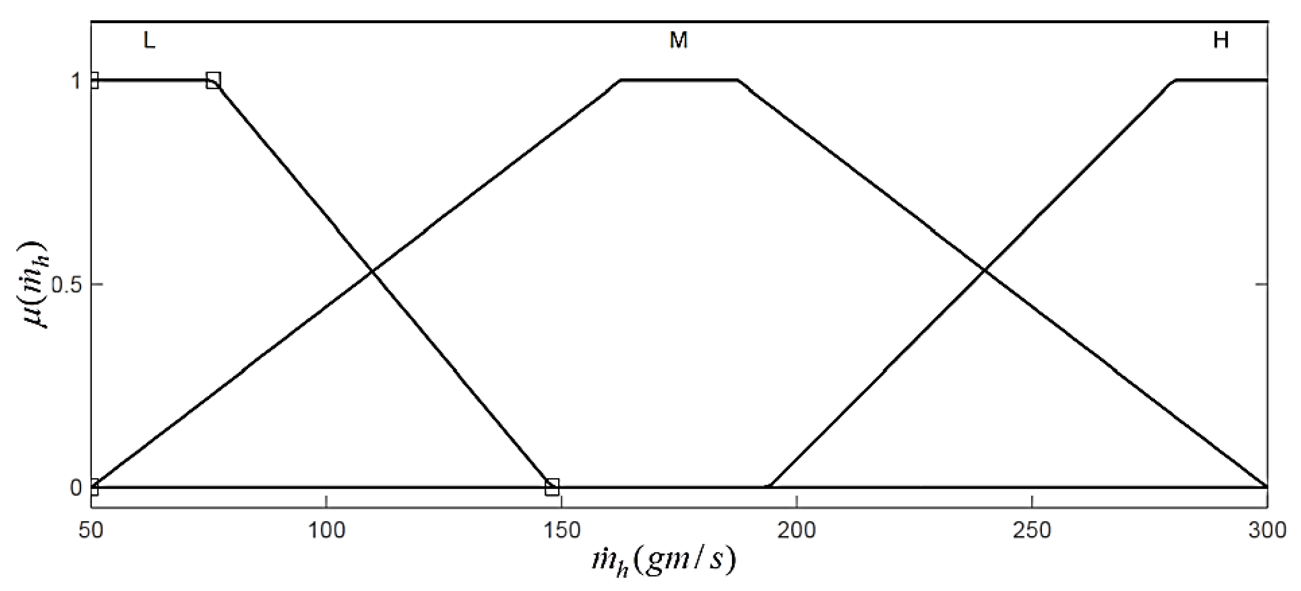
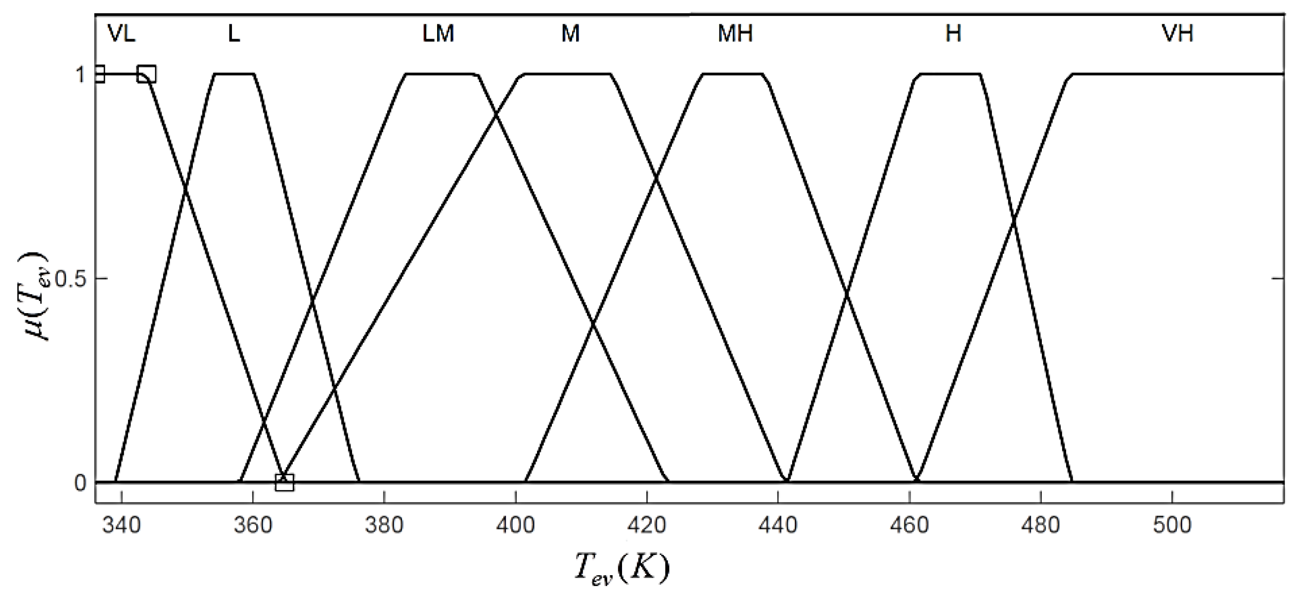
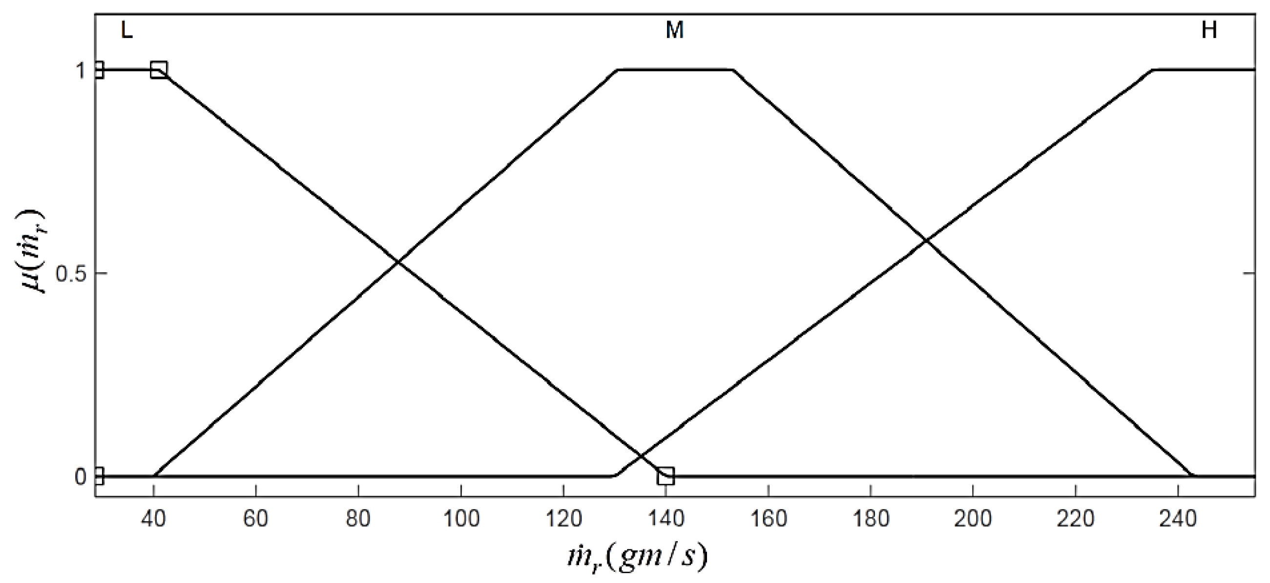
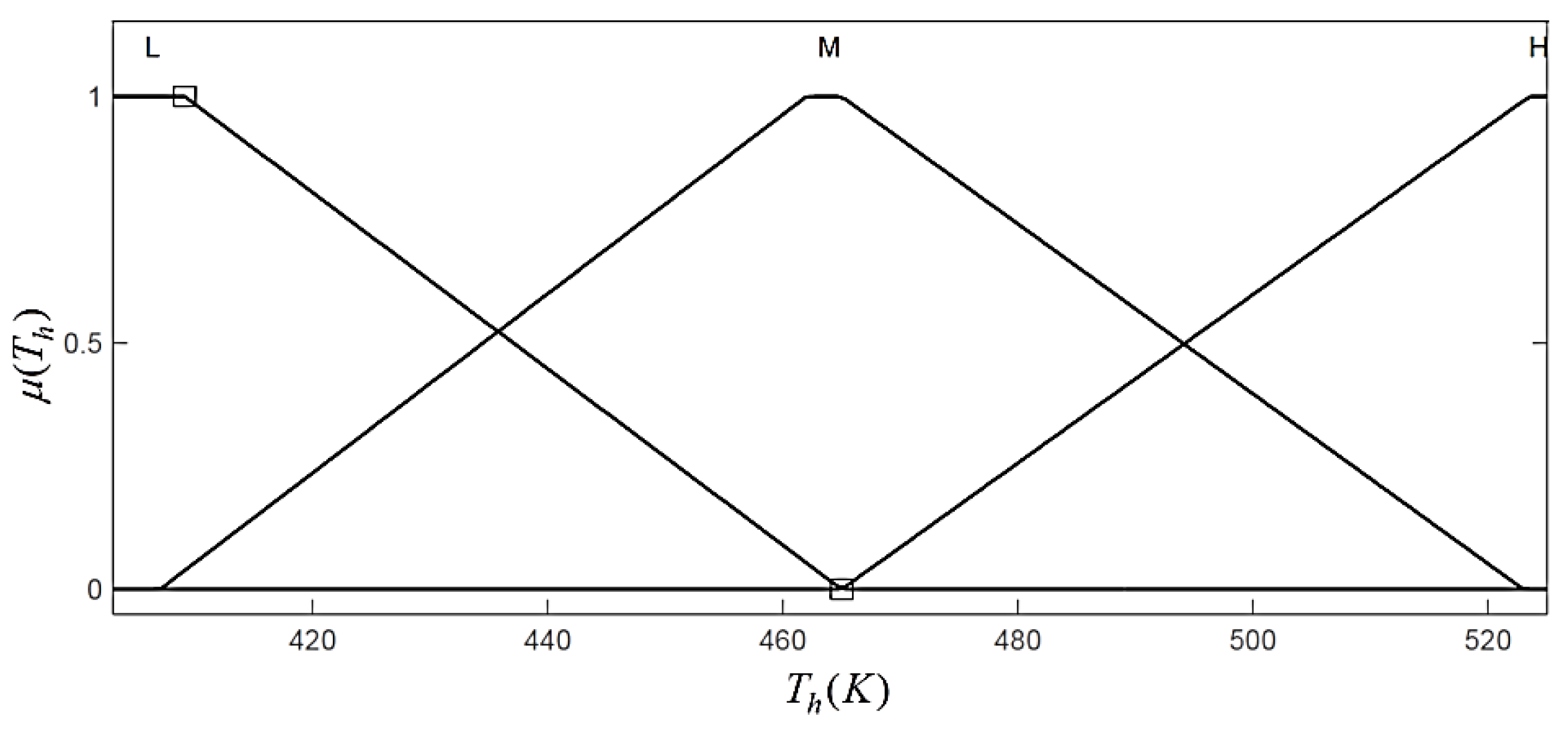
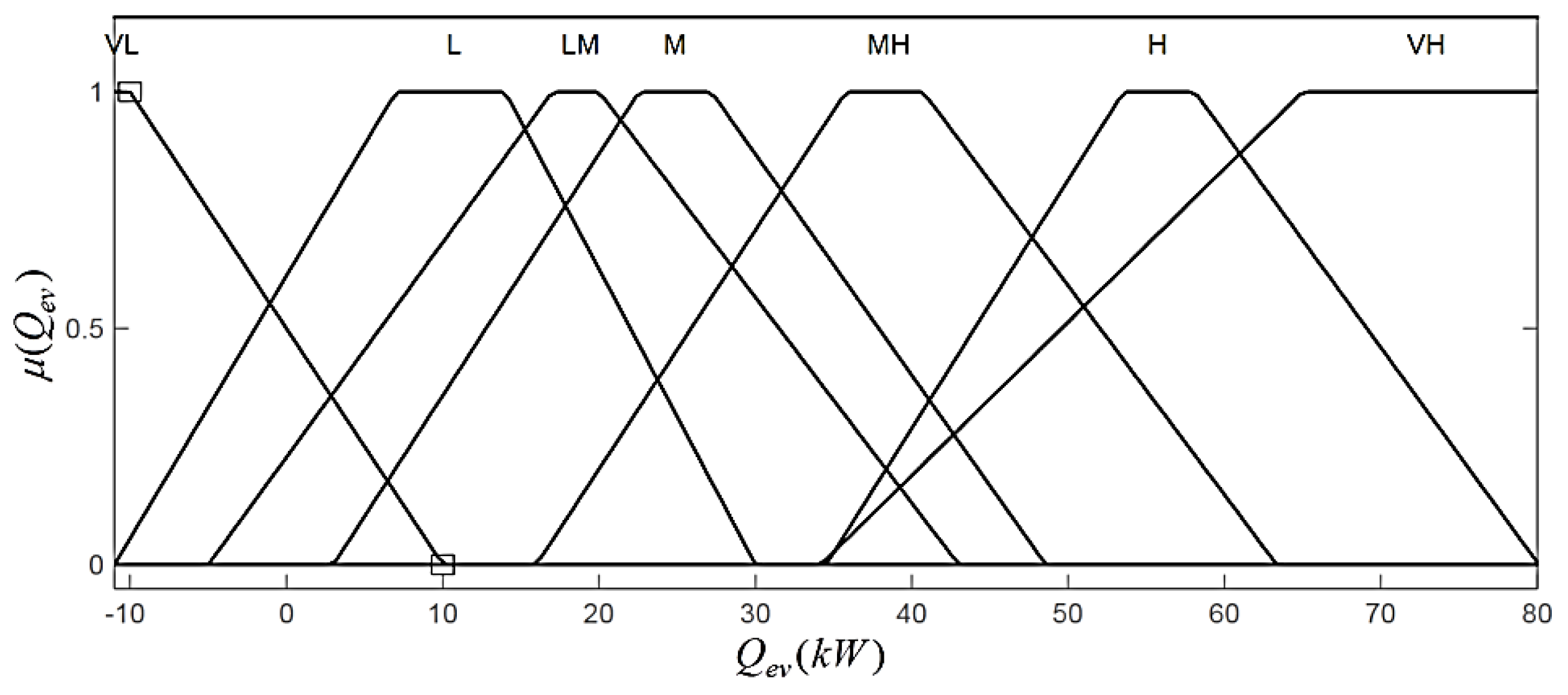
The variable ranges of the fuzzy based evaporator are determined from the input and output profiles and adjusted from the experience of the system as follows:
[28.6 (gm/s), 255 (gm/s)],
[50 (gm/s), 300 (gm/s)],
[403 (K), 525 (K)],
[−11 (kW), 80 (kW)] and
[336 (K), 517 (K)], respectively. Each of these input and output value is called a crisp value. The ranges of these variables are shown in
Figure 14,
Figure 15,
Figure 16,
Figure 17 and
Figure 18.
Figure 14.
Membership functions of refrigerant mass flow rate.
Figure 14.
Membership functions of refrigerant mass flow rate.
Figure 15.
Membership functions of hot fluid mass flow rate.
Figure 15.
Membership functions of hot fluid mass flow rate.
Figure 16.
Membership functions of hot fluid temperature.
Figure 16.
Membership functions of hot fluid temperature.
Figure 17.
Membership functions of evaporator outlet temperature.
Figure 17.
Membership functions of evaporator outlet temperature.
Figure 18.
Membership functions of evaporator power.
Figure 18.
Membership functions of evaporator power.
Step 2: Fuzzification
In this work, the linguistic levels assigned to the input and output variables are as follows: VL: Very Low; L: Low; LM: Low to Medium; M: Medium; MH: Medium to High; H: High and VH: Very High. The linguistic level in fuzzy inference system is termed as membership function. Each input and output of the proposed fuzzy model consists of three and seven membership functions, respectively. The membership functions of each input and output are determined and adjusted by the experience about the system of the designer. In order to obtain a feasible rule bases with high efficiency, all the input and output values were normalized over the interval [0,1], as shown in
Figure 14,
Figure 15,
Figure 16,
Figure 17 and
Figure 18.
L, M and H are assigned as the fuzzy sets of
,
and
which are the inputs of the fuzzy model, and the membership functions of the fuzzy sets are shown in
Figure 14,
Figure 15 and
Figure 16. Similarly, the fuzzy sets assigned to the output variables of the model are VL, L, LM, M, MH, H and VH and are shown in
Figure 17 and
Figure 18.
Step 3: Fuzzy rules and fuzzy inference
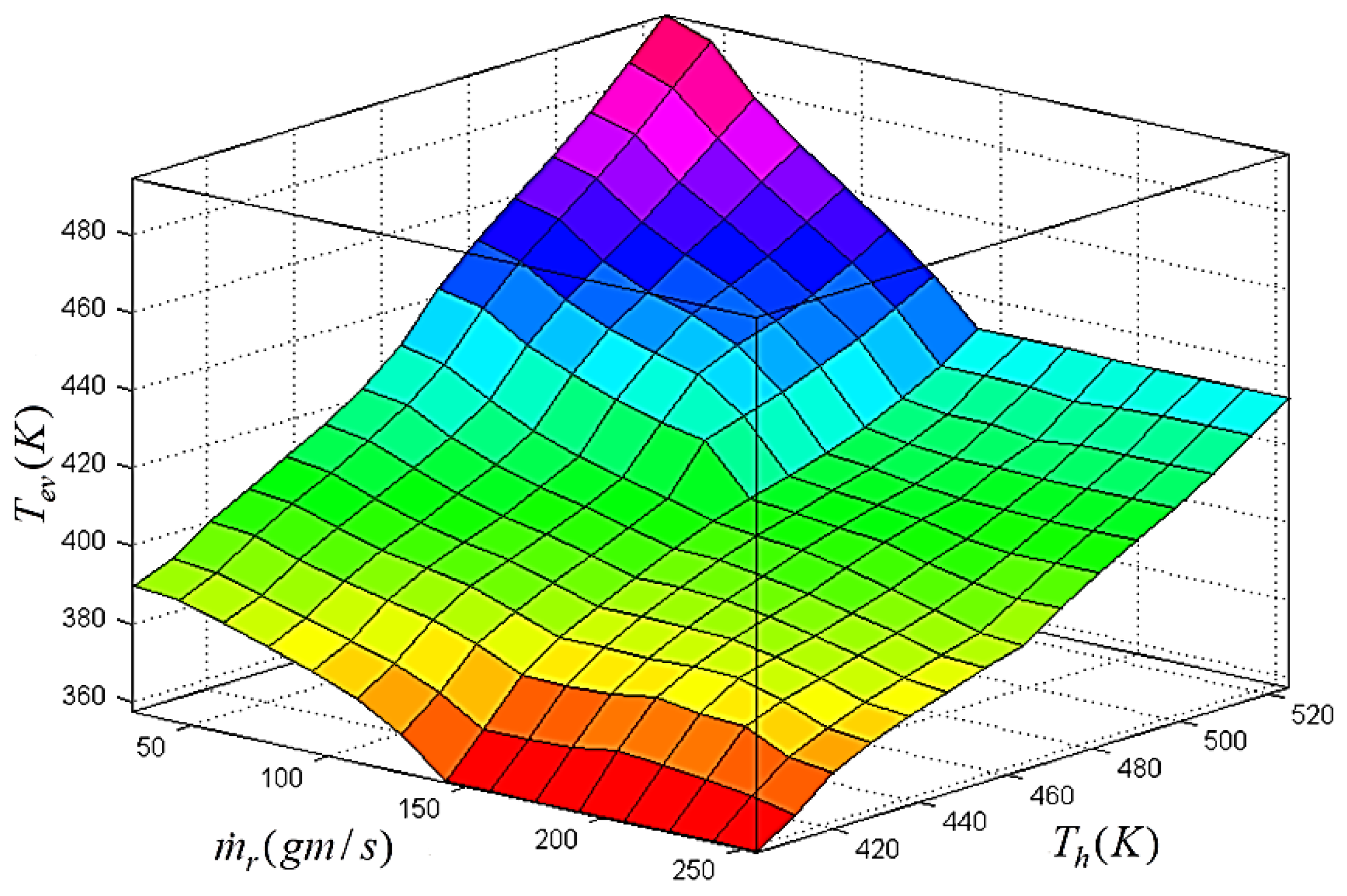
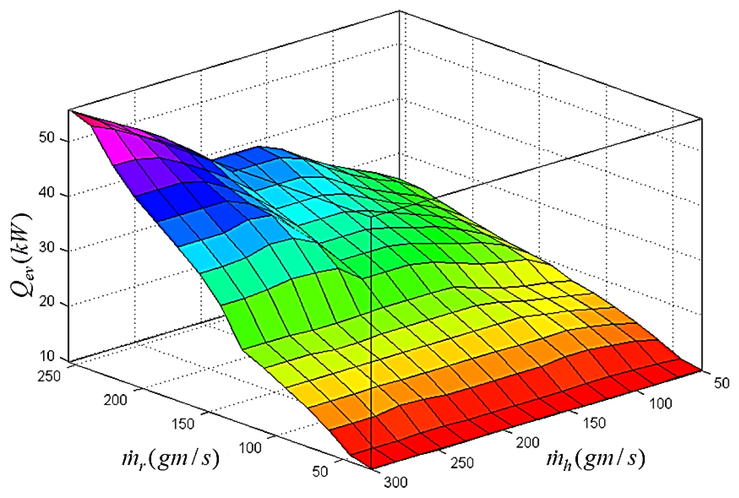
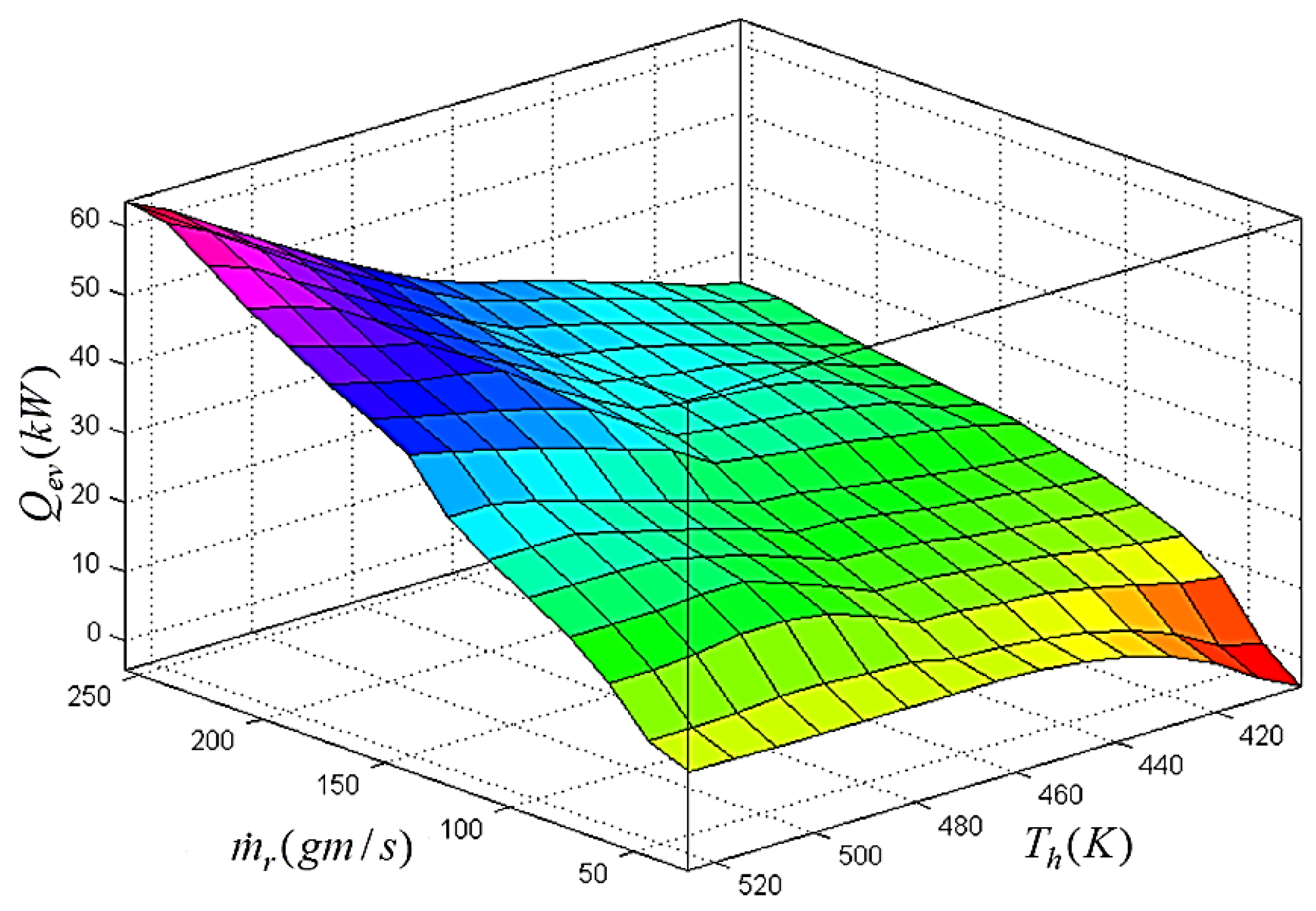
Using the above fuzzy sets of the input and output variables, the fuzzy rules applied in the evaporator model are composed as follows:
where
,
is the number of fuzzy rules,
,
,
,
,
are the
th fuzzy sets of the input and output variables of the fuzzy system. In this research, trapezoidal functions are used as the membership functions, denoted by
μ in
Figure 14,
Figure 15,
Figure 16,
Figure 17 and
Figure 18. The numbers of rules for the fuzzy model are dependent on the number of input membership functions used to define the system. The rules are determined from intuition and knowledge of characteristics of the evaporator and are shown in
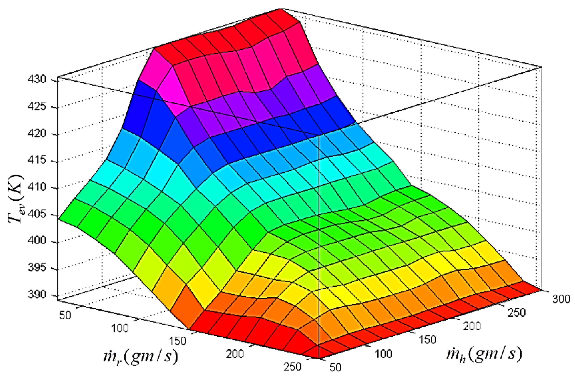
Table 5 and in surfaces in
Figure 19,
Figure 20,
Figure 21 and
Figure 22.
Table 5.
Fuzzy rules for the three inputs and two outputs evaporator model.
Table 5.
Fuzzy rules for the three inputs and two outputs evaporator model.
| Rule number | IF is | AND is | AND is | THEN is | AND is |
|---|
| 1 | L | L | L | LM | VL |
| 2 | L | L | M | M | L |
| 3 | L | L | H | VH | L |
| 4 | M | L | L | VL | L |
| 5 | M | L | M | LM | LM |
| 6 | M | L | H | M | M |
| 7 | H | L | L | VL | LM |
| 8 | H | L | M | LM | M |
| 9 | H | L | H | LM | MH |
| 10 | L | M | L | LM | VL |
| 11 | L | M | M | MH | L |
| 12 | L | M | H | VH | L |
| 13 | M | M | L | L | LM |
| 14 | M | M | M | M | M |
| 15 | M | M | H | MH | MH |
| 16 | H | M | L | L | M |
| 17 | H | M | M | LM | MH |
| 18 | H | M | H | MH | VH |
| 19 | L | H | L | LM | VL |
| 20 | L | H | M | MH | L |
| 21 | L | H | H | VH | L |
| 22 | M | H | L | LM | LM |
| 23 | M | H | M | M | M |
| 24 | M | H | H | H | MH |
| 25 | H | H | L | L | M |
| 26 | H | H | M | LM | H |
| 27 | H | H | H | MH | VH |
Figure 19.
Fuzzy surface for the evaporator outlet temperature with respect to and .
Figure 19.
Fuzzy surface for the evaporator outlet temperature with respect to and .
Figure 20.
Fuzzy surface for the evaporator outlet temperature with respect to and .
Figure 20.
Fuzzy surface for the evaporator outlet temperature with respect to and .
Figure 21.
Fuzzy surface for the evaporator power with respect to and .
Figure 21.
Fuzzy surface for the evaporator power with respect to and .
Figure 22.
Fuzzy surface for the evaporator power with respect to and .
Figure 22.
Fuzzy surface for the evaporator power with respect to and .
In this work, the MAX-MIN fuzzy reasoning method is used to obtain the output from the inference rule and present input. For given a specific input fuzzy set
in
, the output fuzzy set
in
for
is computed through the inference system as follows:
The output membership functions for is calculated similarly.
Step 4: Defuzzification
The centroid defuzzification method [
33] is used in this paper to convert the aggregated fuzzy set to a crisp output value
from the fuzzy set
in
. This work computes the weighted average of the membership function or the centre of gravity (COG) of the area bounded by the membership function curves:
The crisp value of and were calculated using the above expression.
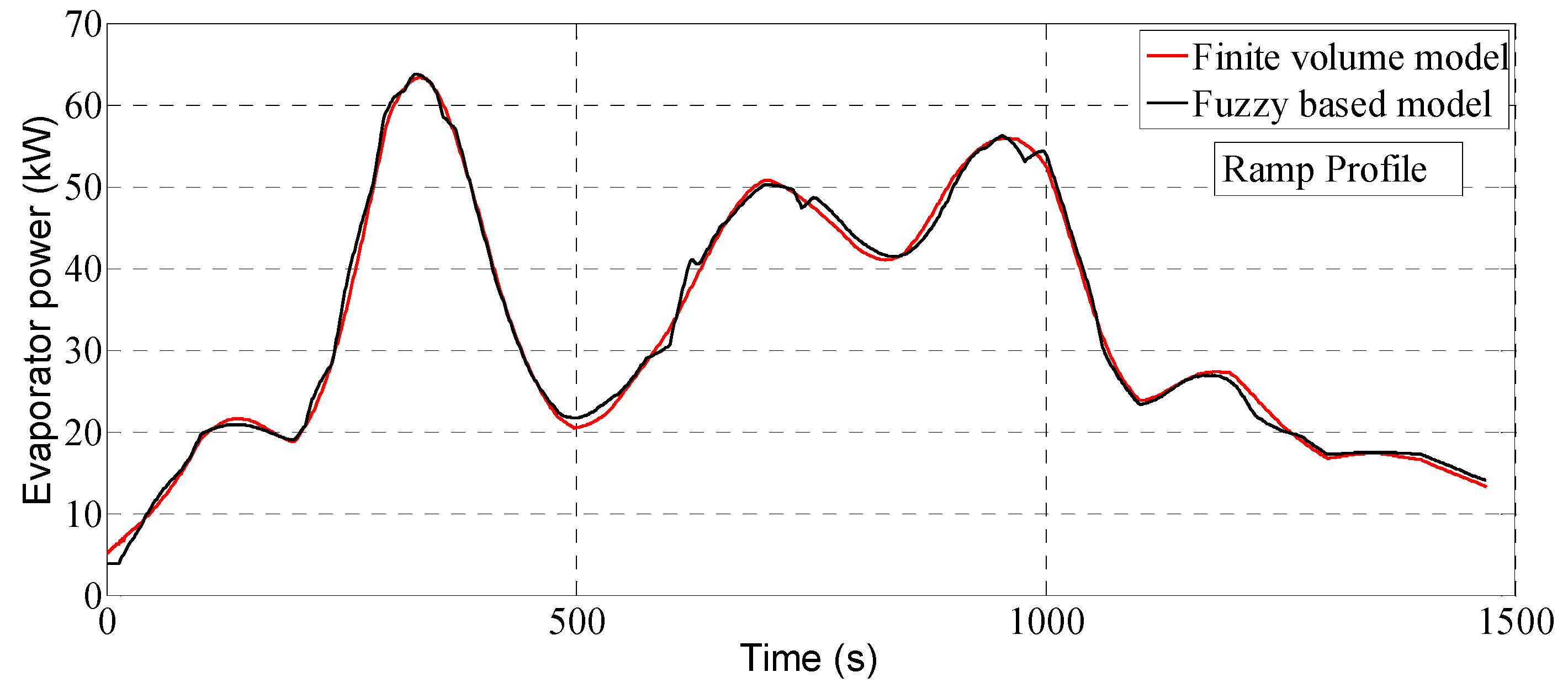
Simulation Results of Fuzzy Based Evaporator Model
The performance of the fuzzy model was investigated with the same heat source and input profiles as the finite volume method. The outputs of the fuzzy evaporator model compared with those of the finite volume method with respect to the ramp input profile are presented in
Figure 23 and
Figure 24. As shown in
Figure 23, the fuzzy based model can be used to predict the evaporator power although there are still some small deviations compared with the FV method. The following indicators are used to evaluate the performance of the proposed fuzzy based model compared with the finite volume method:
where
is the estimated time series,
is the actual time series and
is the total number of data sets.
Figure 23.
Prediction of the evaporator power with respect to ramp profile.
Figure 23.
Prediction of the evaporator power with respect to ramp profile.
Figure 24.
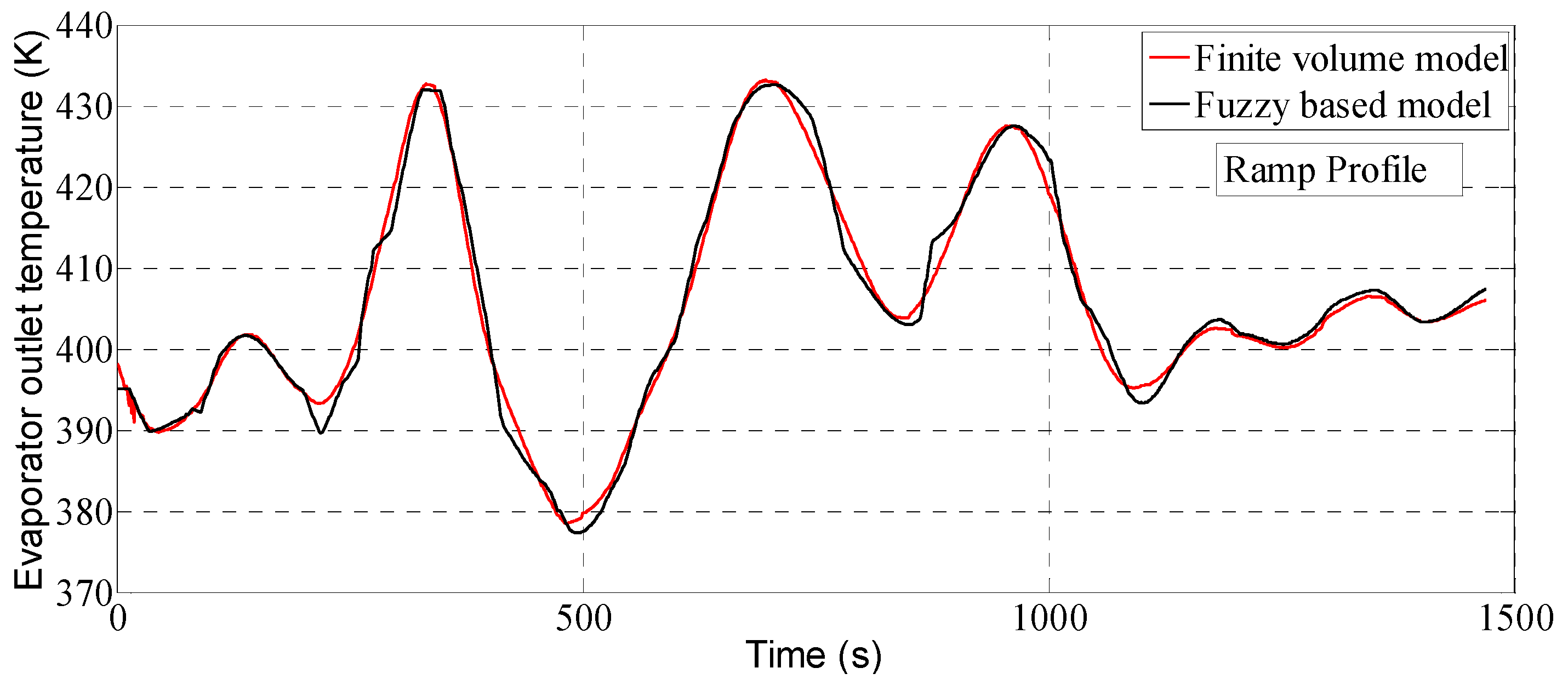
Prediction of the evaporator outlet temperature with respect to ramp profile.
Figure 24.
Prediction of the evaporator outlet temperature with respect to ramp profile.
The congruency of the fit between the model outputs of these two methods was also evaluated as follows:
Table 6 shows the RMSE and fitness values of the fuzzy based evaporator model compared with the finite volume method with respect to difference input profiles. The RMSE value of the evaporator power
for the ramp profile is 0.95 kW; while the congruency of the fit of the fuzzy model is 93.68%. Similarly, the evaporator outlet temperature of the fuzzy based model was compared to that of a finite volume model which is shown in
Figure 24. The RMSE and congruency of the fit of the fuzzy model output for ramp profile are 1.48 K, and 89.16%, respectively.
Table 6.
Performance of the fuzzy based evaporator model.
Table 6.
Performance of the fuzzy based evaporator model.
| Performance Indicator | RMSE | Fitness (%) | Simulation Time |
|---|
| -Ramp Profile | 0.95 (kW) | 93.68 | Almost instantly (<1 s) |
| -Ramp Profile | 1.48 (K) | 89.16 |
| -Random Profile | 0.92 (kW) | 92.31 | Almost instantly (<1 s) |
| -Random Profile | 3.02 (K) | 87.00 |
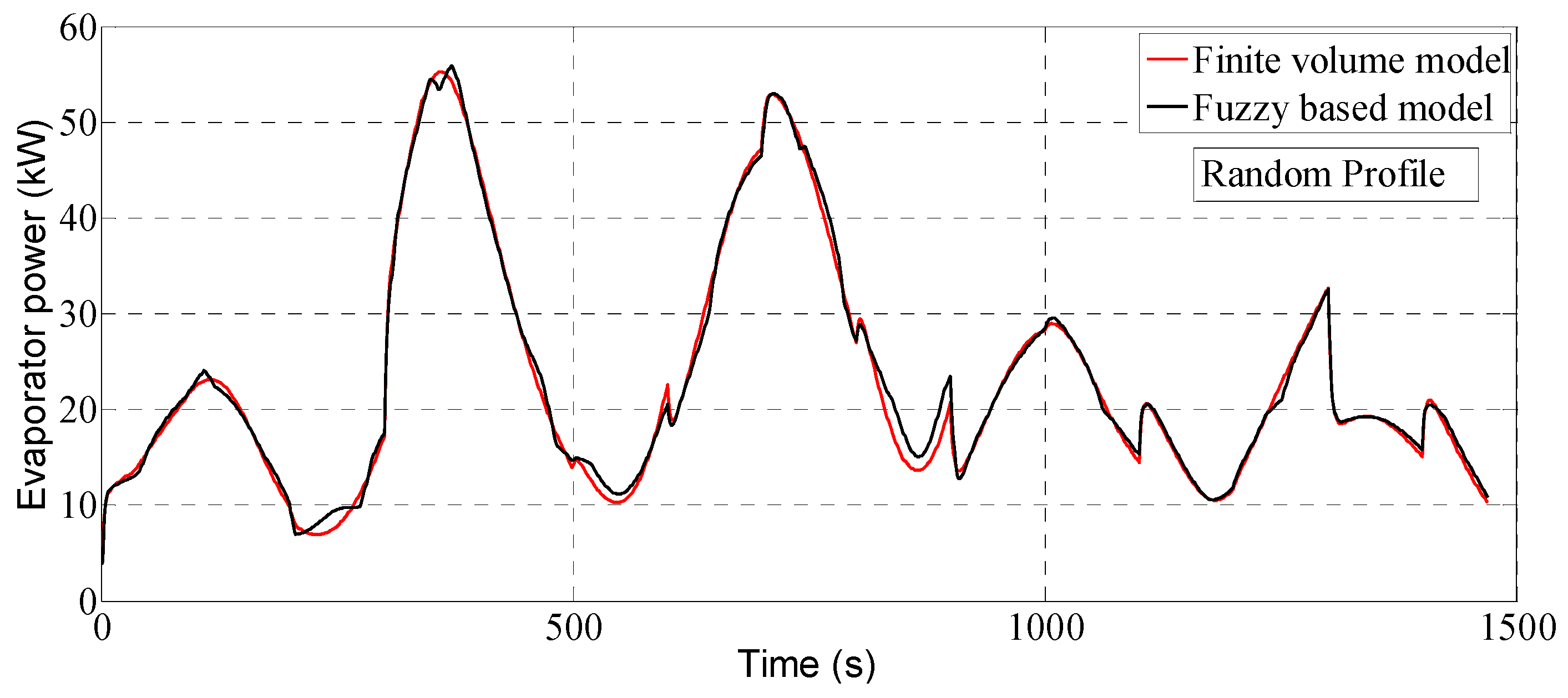
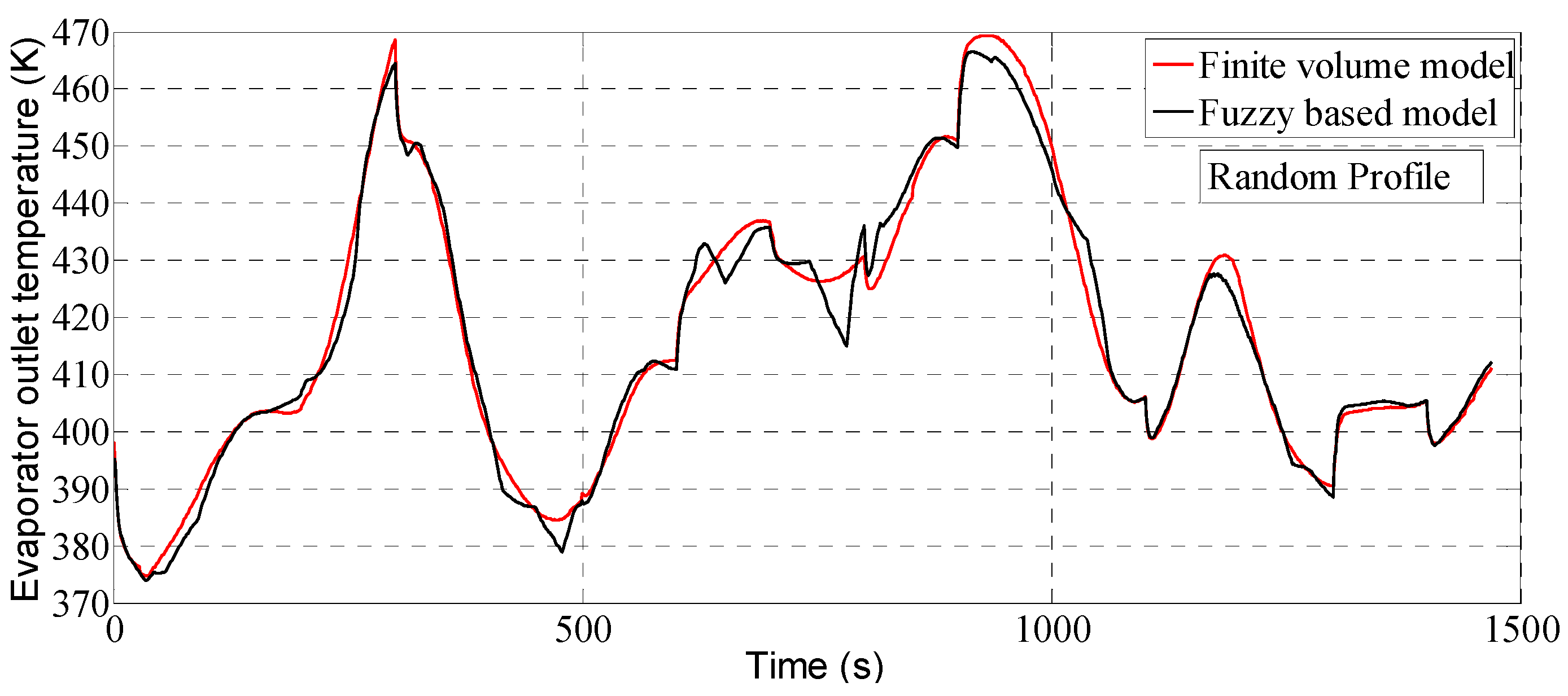
Figure 25 and
Figure 26 show the evaporator outputs of the fuzzy and FV model with respect to the random mass flow rate profile. The RMSE and data fitness values are 0.92 kW and 92.31% for the evaporator power, 3.02 K and 87% for the evaporator outlet temperature, respectively. It can be seen from the
Figure 25 and
Figure 26 that the fuzzy model can accurately forecast the evaporator outputs within all the operation ranges. However, since the membership functions and fuzzy rules were not optimized during the design of the fuzzy based evaporator model, there are small errors at some areas as shown in
Figure 23,
Figure 24,
Figure 25 and
Figure 26. These discrepancies can be improved by adjusting and optimizing the membership functions and their linguistic levels based on the knowledge about the evaporator operation.
Figure 25.
Prediction of evaporator power with respect to random profile.
Figure 25.
Prediction of evaporator power with respect to random profile.
Figure 26.
Prediction of evaporator outlet temperature with respect to random profile.
Figure 26.
Prediction of evaporator outlet temperature with respect to random profile.
The fuzzy based model outputs for both profiles are obtained in less than 1 second. On the other hand, the computation times of the FV model for the ramp and random profiles are 13,870 and 14,826 s, respectively. Comparing with the FV method, the proposed fuzzy based model saves a large amount of computation time as it can calculate the model outputs almost instantly.


