Dynamic Modeling of the Solar Field in Parabolic Trough Solar Power Plants

Abstract

Parabolic trough solar power plants use a thermal fluid to transfer thermal energy from solar radiation to a water-steam Rankine cycle in order to drive a turbine that, coupled to an electrical generator, produces electricity. These plants have a heat transfer fluid (HTF) system with the necessary elements to transform solar radiation into heat and to transfer that thermal energy to the water-steam exchangers. In order to get the best possible performance in the Rankine cycle and, hence, in the thermal plant, it is necessary that the thermal fluid reach its maximum temperature when leaving the solar field (SF). Also, it is mandatory that the thermal fluid does not exceed the maximum operating temperature of the HTF, above which it degrades. It must be noted that the optimal temperature of the thermal fluid is difficult to obtain, since solar radiation can change abruptly from one moment to another. The aim of this document is to provide a model of an HTF system that can be used to optimize the control of the temperature of the fluid without interfering with the normal operation of the plant. The results obtained with this model will be contrasted with those obtained in a real plant.

1. Introduction

Solar radiation can be exploited in several ways. While photovoltaic (PV) systems use luminous solar radiation to produce electricity, thermoelectric solar plants use thermal radiation. There are different technologies that take advantage of the solar thermal energy. They can be classified depending on the temperatures they can reach. In [1], differences between these technologies are shown. Parabolic trough collector (PTC) technology is one of the most mature and, for that reason, the most implanted one worldwide. They use a heat transfer fluid (HTF) that flows inside several absorber pipes placed in the focal axis of a set of mirrors. These mirrors focus the solar radiation over the pipes in such a way that the HTF absorbs the thermal energy of the sun.

Although some of the older concentrated solar power (CSP) plants do not have any sort of thermal energy storage, the fact is that during the last years several installations with a thermal energy storage (TES) system have appeared, as well as papers dealing with different methods to store thermal energy and with how to control such storage [1,2,3,4,5,6].

Figure 1 shows a schematic of a solar thermal power plant of PTCs with a TES system. This thermoelectric solar plant works basically like a conventional thermal one. It consists of a generator steam train that, thanks to the contribution of thermal energy, turns liquid water into steam. This steam drives a turbine coupled to an electric generator that produces electricity.

Figure 1. Schematic of a parabolic trough collector (PTC) solar thermoelectric plant.

Figure 1. Schematic of a parabolic trough collector (PTC) solar thermoelectric plant.

In order for these plants to be able to use solar thermal radiation, they have a subsystem named solar field (SF). This system absorbs the solar radiation, extracts its thermal energy and transports it to the rest of the subsystems, such as the steam generator (SG) and the TES. A HTF crosses the SF absorbing thermal energy from the sun and transferring it to the rest of the plant.

The main objective is to achieve as high a fluid temperature as possible at the output of the SF, but without exceeding the maximum operating temperature of the fluid. The purpose of the control of the heating process is to define a set point temperature and guarantee that, if the temperature at the output of the SF tends to rise above that set point, the control causes the mass flow of the fluid to rise and vice versa. In order to optimize this control system, an accurate model of the process to be controlled is required, since the power plant will not stop production so that different control strategies can be tested. The goal of this paper is to produce a simple yet accurate version of such a model.

2. Results and Discussion

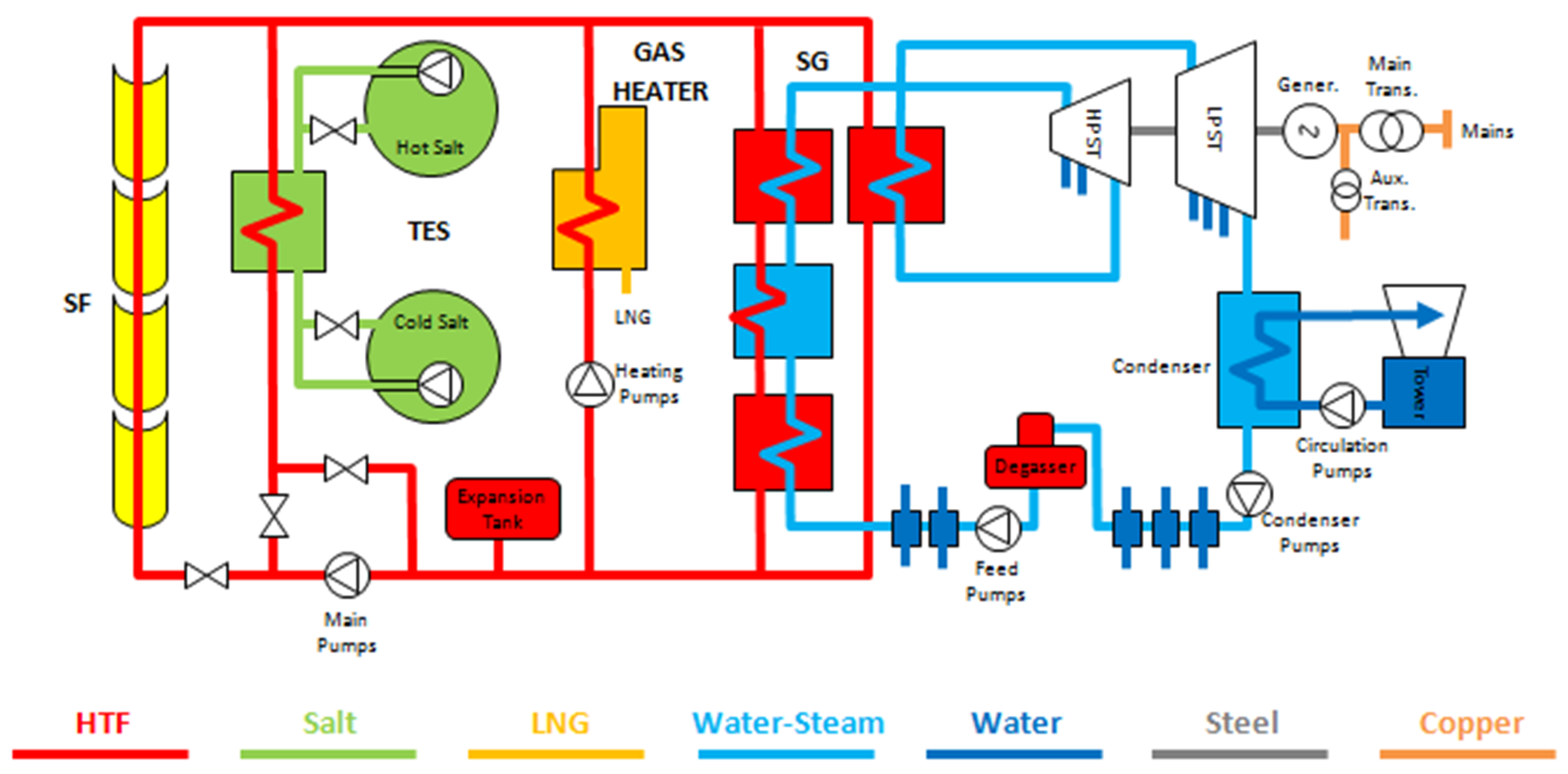
2.1. Description of the Solar Field (SF)

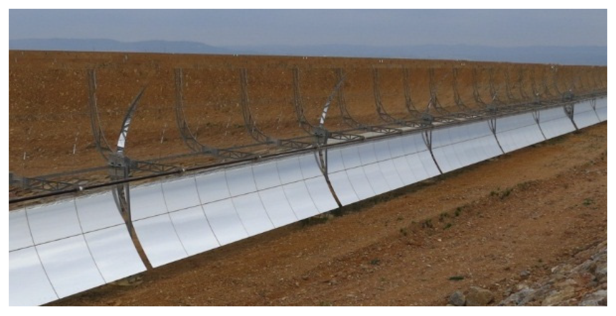
In order to adequately model the thermal-fluid heating process, it is mandatory to understand the main elements of the HTF system. This system contains several solar collector assemblies (SCA), Figure 2 formed by solar collector elements (SCE), Figure 3. Each SCE has mirrors (28 mirrors in Figure 3) as well as absorber pipes arranged in such a way that the SCE is parabolic-trough shaped and the pipes are placed in its focal axis.

Depending on the solar thermal plant, the SCA may have six, eight or 12 SCEs. The dynamic model developed in this paper is based on the HTF system of the PTC solar plant “La Africana”, located in Cordoba, Spain. In the SF of “La Africana”, each SCE has three absorber tubes arranged in series and each SCA is formed by 12 SCEs.

SCAs are arranged in series forming loops. These loops can be U-shaped or W-shaped. In the model described, U-shaped loops with four SCAs each are considered.

Figure 2. Solar collector assembly (SCA).

Figure 2. Solar collector assembly (SCA).

Figure 3. Solar collector element (SCE) with 28 mirrors and three absorber pipes.

Figure 3. Solar collector element (SCE) with 28 mirrors and three absorber pipes.

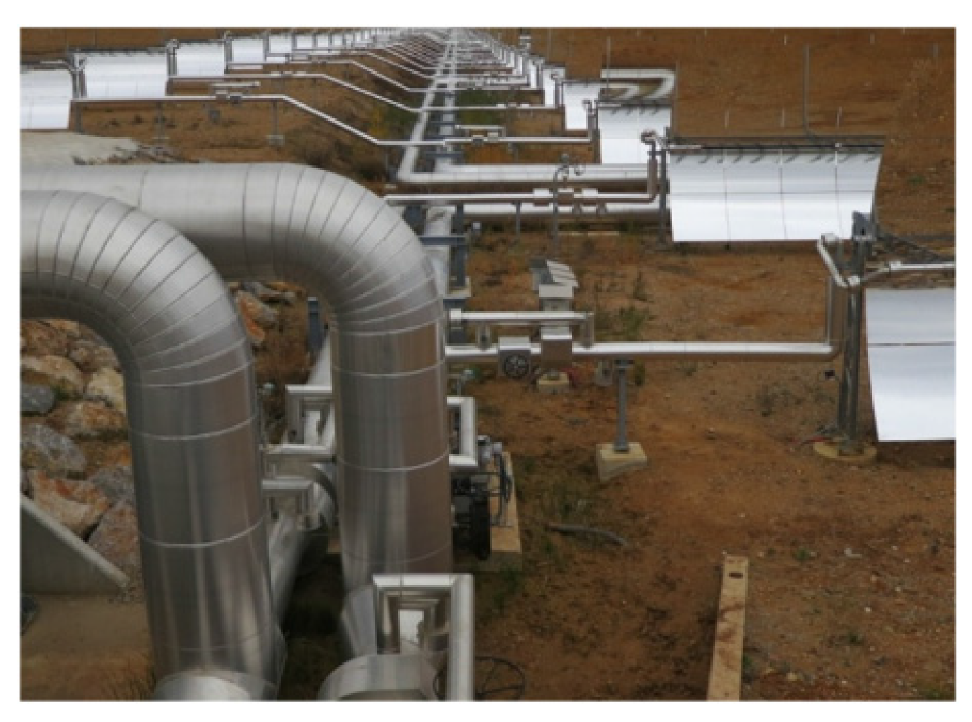
The beginning of the loop is linked to a large diameter pipe (cold header) that contains cold HTF (HTF that has not been heated by the solar radiation yet). The end of the loop is linked to another large diameter pipe (hot header) in such a way that, once the fluid coming out of the loops has been heated, it is transported to the steam generator system (SGS) and/or the TES system, depending on the operation mode. Figure 4 shows one of these loops.

Figure 4. U-Shaped loop in PTC solar plants.

Figure 4. U-Shaped loop in PTC solar plants.

The elements included in the HTF system, also referred to as SF, modeled in this paper has 168 loops with 4 SCA per loop. Each SCA consists on 12 SCE that contains 3 absorber pipes. Therefore, this HTF systems has 24.192 absorber pipes transporting the fluid.

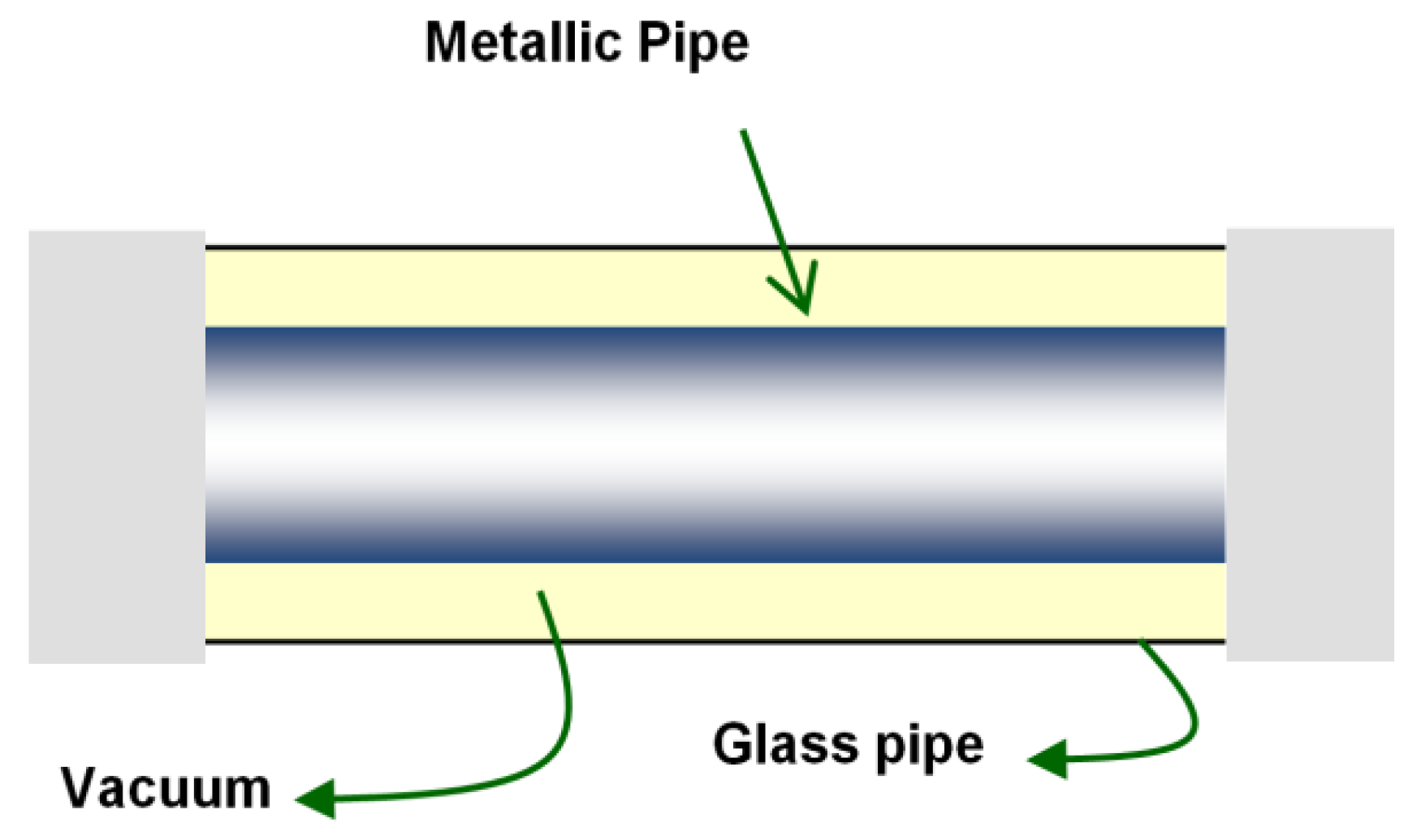
The most important elements to take into account in the modeling of this process are the absorber pipes, shown in Figure 5 They are in charge of absorbing the solar radiation and turning it into thermal energy. Thanks to the fluid that flows through them, they also transport that thermal energy to the rest of the plant where needed.

Figure 5. Headers.

Figure 5. Headers.

They consist of two concentric pipes. The inner one is metallic with a blue film to minimize radiation thermal losses, whereas the outer pipe is made of glass. Vacuum is created between them in order to avoid convention and conduction thermal losses. Figure 6 shows the main parts of an absorber pipe.

Figure 6. Absorber pipe.

Figure 6. Absorber pipe.

2.2. Description of the Heat Transfer Fluid (HTF)-Heating Process

The solar radiation is reflected by the mirrors over the absorber pipes, thus heating the HTF. A comparative study of the different thermal fluids most currently used in PTC power plants (oil, molten salt and water steam) is presented in [7]. The authors conclude that direct steam generation is more efficient than the other two. In spite of that, and although other alternatives are being studied [8,9,10,11,12,13,14], most of the PTC plants use some sort of synthetic oil, mainly due to its lower freezing point (around 12 °C) when compared to other HTFs.

According to the literature, there are different kinds of fluids that have been or are being analyzed to be used as HTF. One of them is molten salt. Taking into account that they are used to store thermal energy in the TES, it would be relatively easy to use it also in the SF. The main problem is its high freezing point (around 140 °C). Due to the small internal diameter of the absorber pipes, having part of the molten salts freeze would cause blockages that could cause the pipes to break. Other installations use direct steam generators (DGS) instead, in which water acts as HTF. The main advantages of this technology are its lower thermal losses and, therefore, its higher cycle efficiency. Its drawbacks are the higher pressures required and the more complex control needed. These drawbacks are also present in installations that use gas and air as HTF. Two new research lines are emerging nowadays: nanofluids and ionic fluids. The first one consists of adding metallic nanoparticles or carbon nanotubes in order to improve its optical and thermal properties. Ionic fluids are very promising. They are formed by joining anions and cations so that they can result in billions of different ionic fluids for multiple applications.

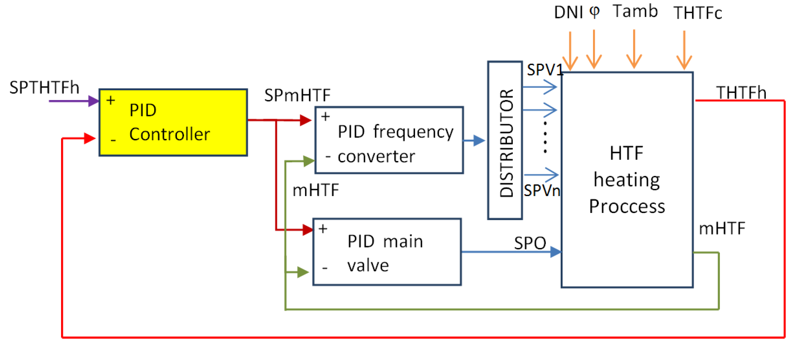
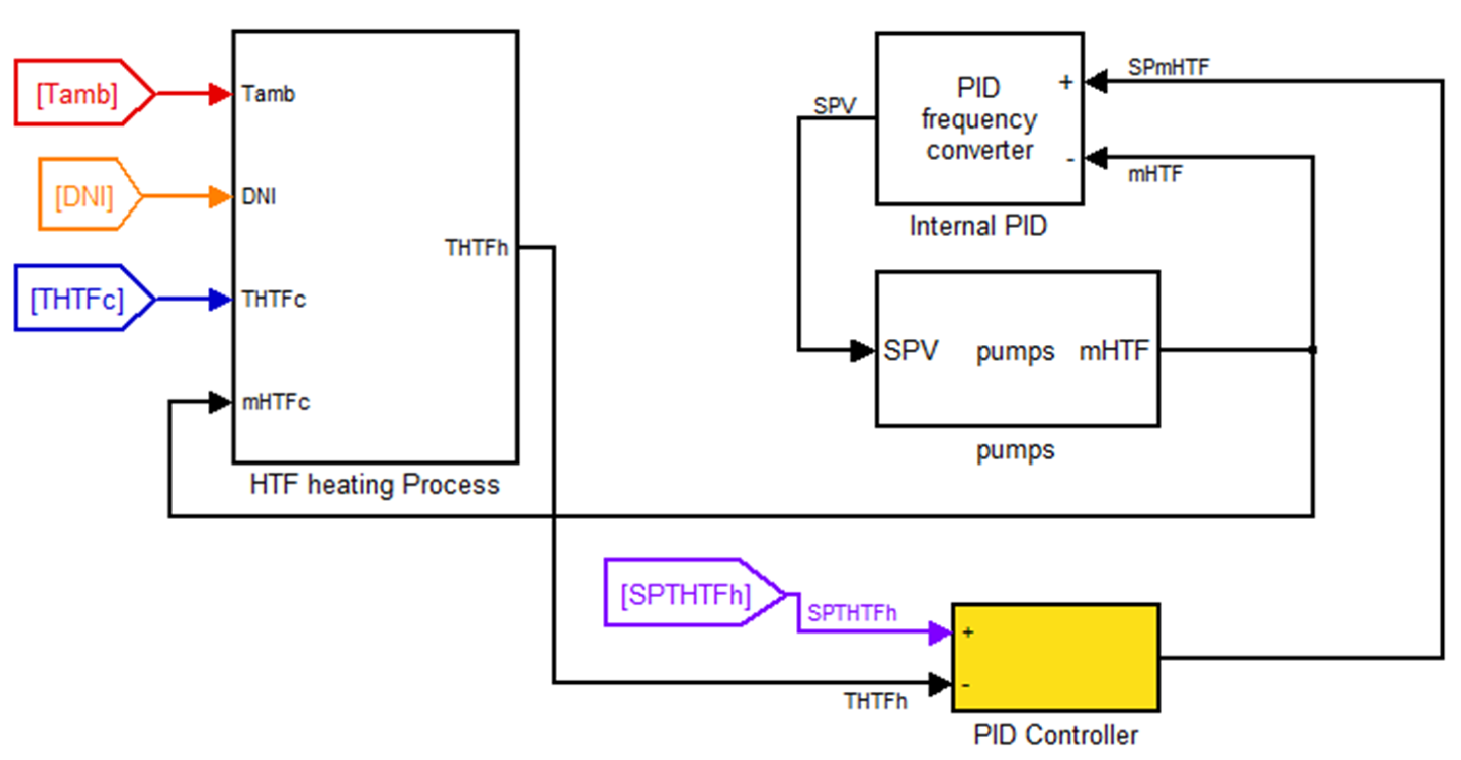
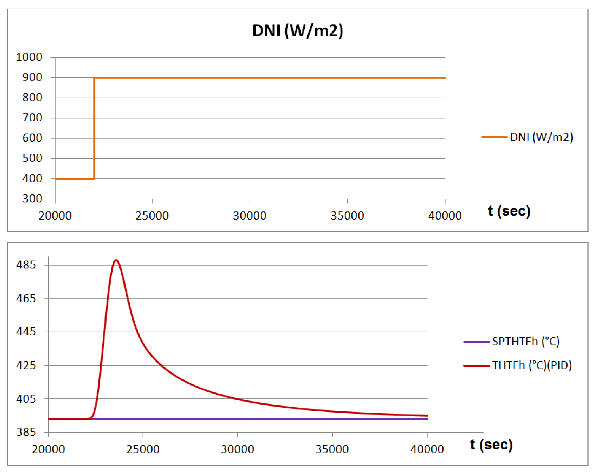
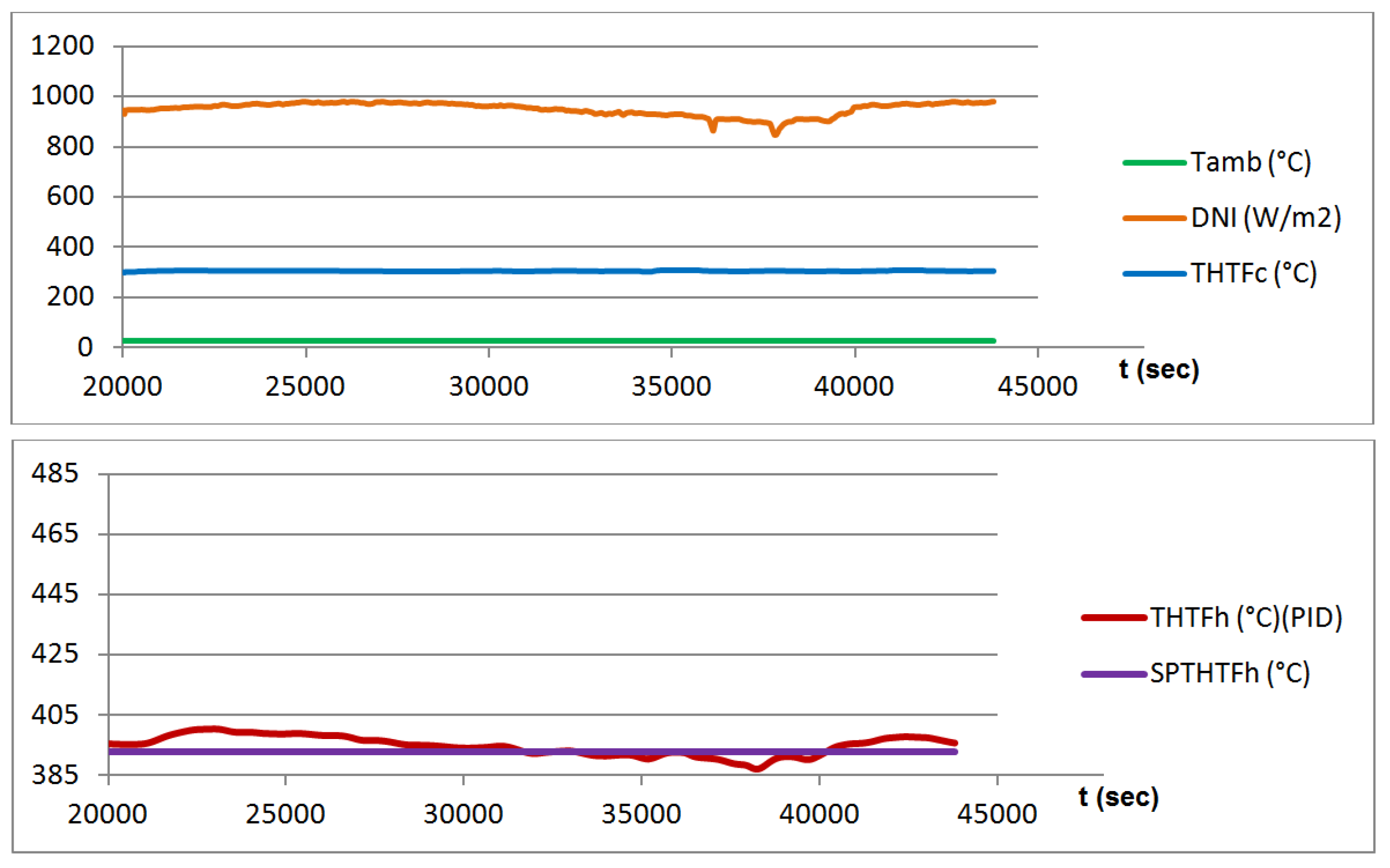
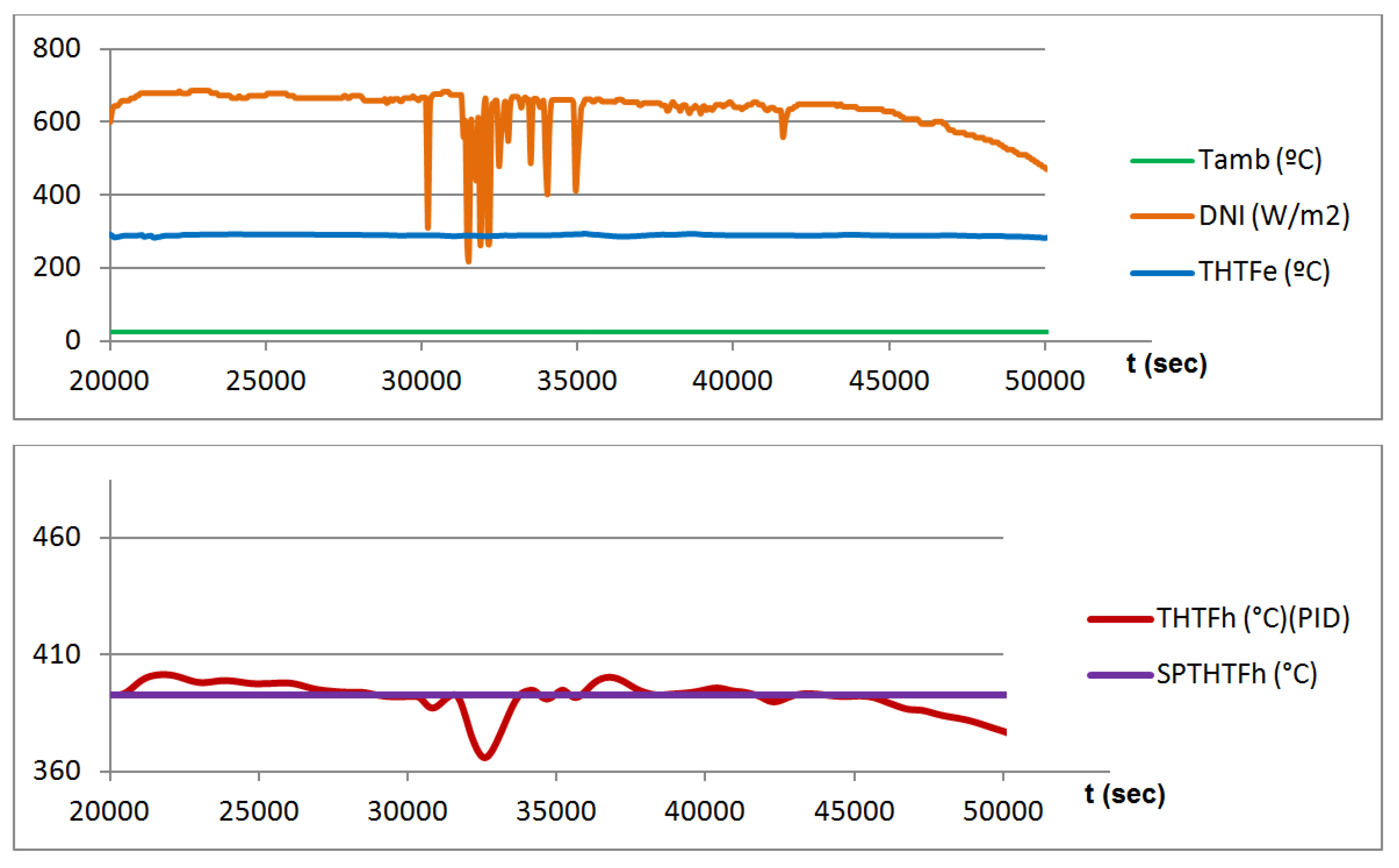
Using synthetic oil as HTF also has drawbacks, the main one being its maximum operation temperature, which is around only 400 °C in the best-case scenario. This critical point can be easily exceeded when direct solar irradiation (DNI) is high. Given that solar radiation is a phenomenon that can vary widely in a short space of time, a good regulation method is necessary. This method should allow the oil to leave the SF with the highest possible temperature while, at the same time, preventing the oil from exceeding its maximum operating point.

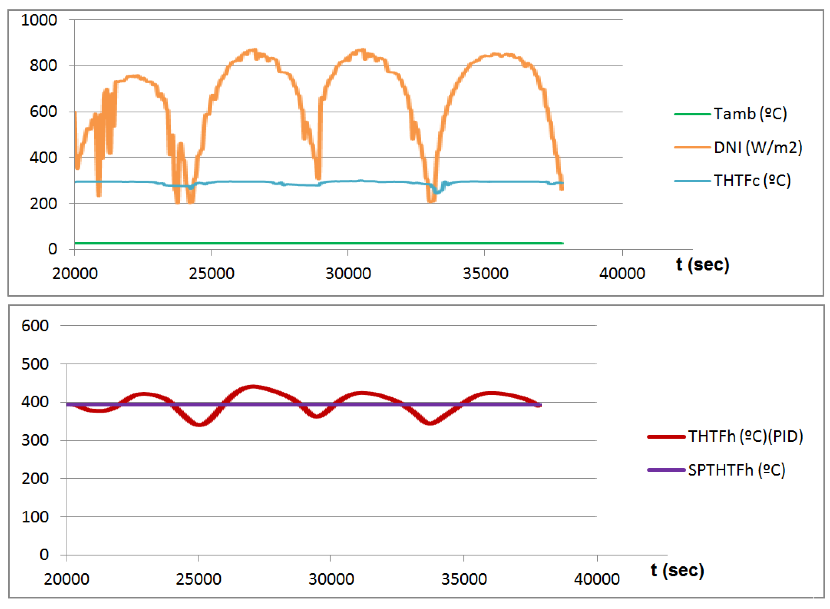
To meet this goal, the control method varies the mass flow of the fluid in such a way that, if the oil temperature exceeds a given set point (393 °C in the case considered), the mass flow will increase. Thus, the time the fluid stays in the SF will be shorter and its temperature will drop. Similarly, if the oil temperature is below the set point, the mass flow must be reduced. Table 1 and Table 2 show all the variables (perturbations, input, output and control variables) involved in the HTF-heating process:

Table 1. Input, output and control variables of the HTF-heating process.

Variable	Acronym	Description
Input	THTFc	Heat transfer fluid (HTF) temperature at the input of the solar field (SF) (°C)
Output	THTFh	HTF temperature at the output of the SF (°C)
Control	${\dot{m}}_{\text{HTF}}$	HTF mass flow (kg/s)

Table 1. Input, output and control variables of the HTF-heating process.

Variable	Acronym	Description
Input	THTFc	Heat transfer fluid (HTF) temperature at the input of the solar field (SF) (°C)
Output	THTFh	HTF temperature at the output of the SF (°C)
Control	${\dot{m}}_{\text{HTF}}$	HTF mass flow (kg/s)

Table 2. Perturbations of the HTF-heating process.

Perturbations	Description
Direct solar irradiation (DNI)	Direct normal irradiation (W/m2)
φ	Angle of incidence (°)
Tamb	Ambient temperature (°C)

Table 2. Perturbations of the HTF-heating process.

Perturbations	Description
Direct solar irradiation (DNI)	Direct normal irradiation (W/m2)
φ	Angle of incidence (°)
Tamb	Ambient temperature (°C)

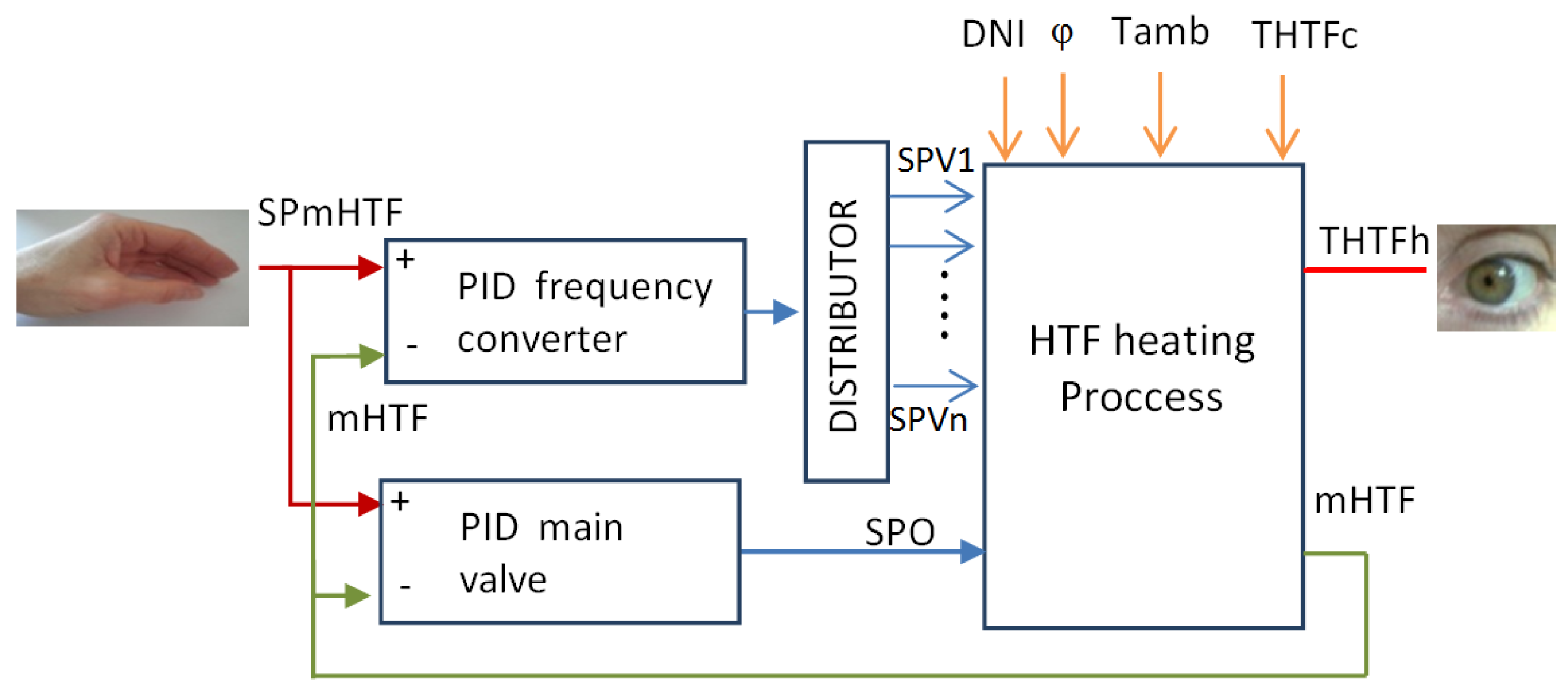
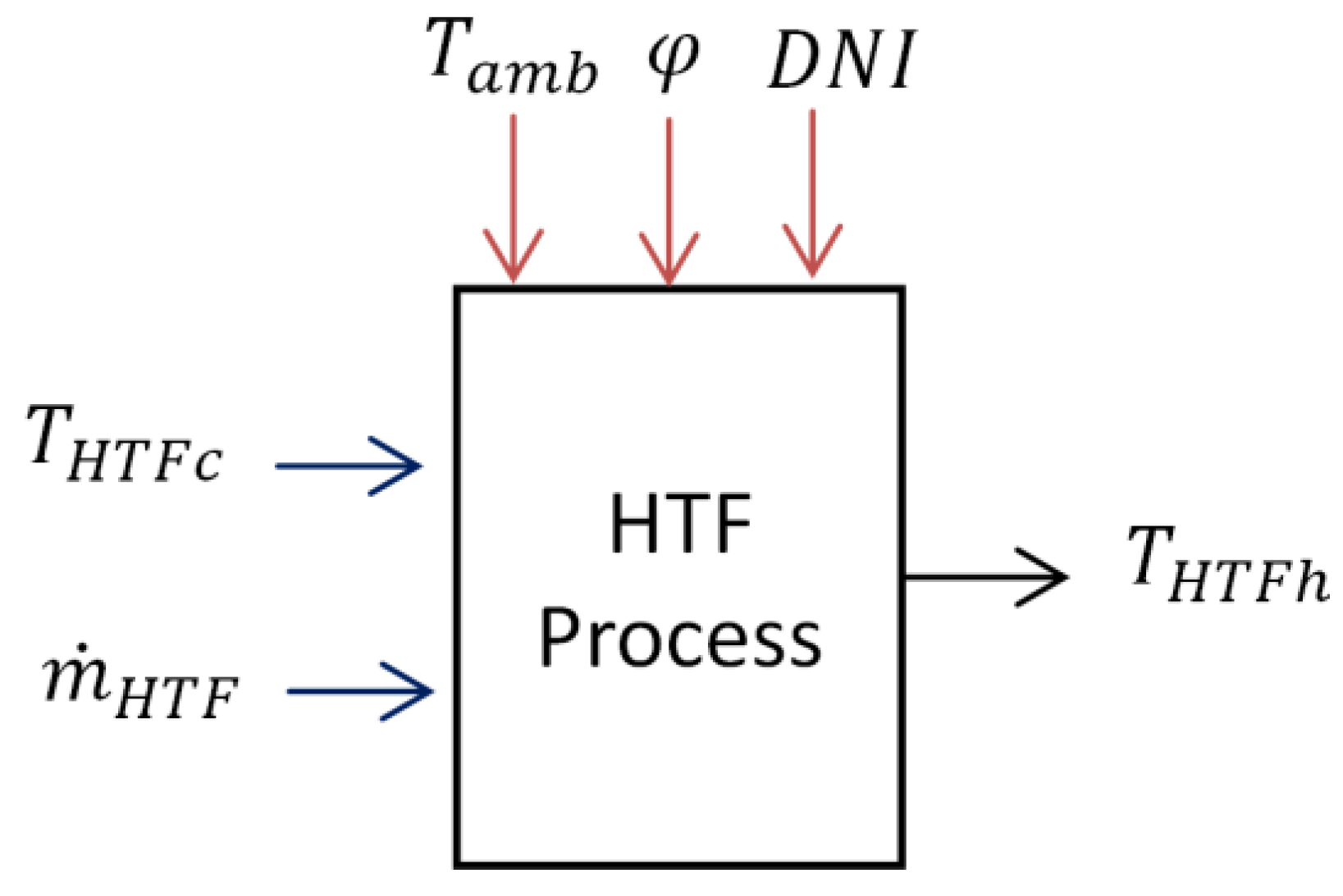
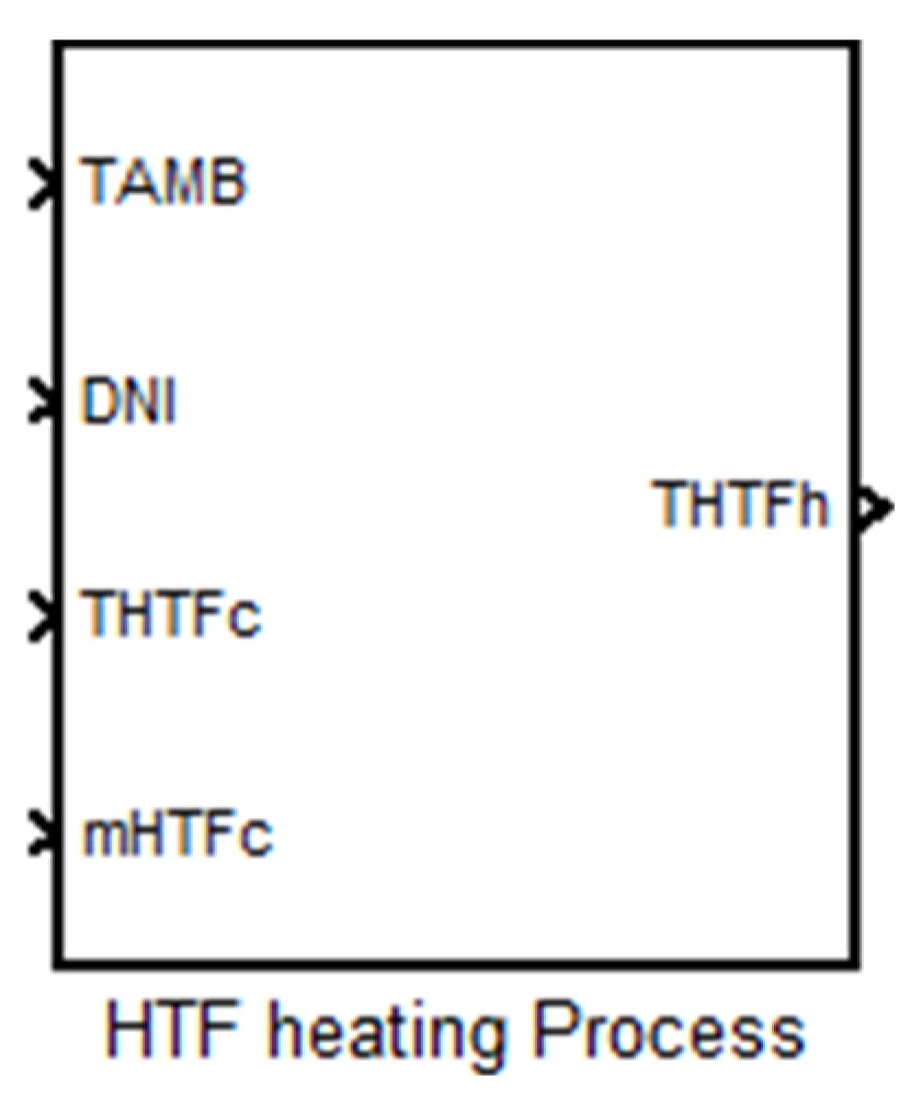
Figure 7 shows the block diagram that represents the process described above.

Figure 7. Heat transfer fluid (HTF)-heating process model.

Figure 7. Heat transfer fluid (HTF)-heating process model.

The goal of this work is to obtain a simple, accurate and dynamic model that allows designers to optimize the control of this process.

2.3. Modeling of the HTF-Heating Process

Several models of different parts of the PTC thermoelectric plants have been developed in the last years. In [15], a mathematical model is described that compares the quasi-dynamic test (QDT) and the steady-state test (SST) in five different types of collectors. In [16], the authors present a dynamic model for the collector field and a steady-state model for the power plant; this paper is based on a real PTC solar plant and the whole plant has been mathematically modeled. In [17] models for different geometries and insulation materials with different thicknesses have been carried out in order to select the best one for high temperature processes; in this paper, all the models are numerically compared and, hence, absolute values are not provided. A paper written by one of the main manufacturers of solar absorber pipes [18] explains all the thermal exchanges between the different parts or elements that form a pipe; this paper is a good starting point to develop the dynamic model of the HTF-heating process. In reference [19], the authors established a computational fluid dynamics (CFD) model to calculate the temperature profile on the wall of the absorber tubes of DSG plants. The authors of [20] compare three different models of absorber pipes: a one- and a two-dimensional analytical model and a three-dimensional one using finite-element techniques.

It must be said that most of these references model the absorber pipes in order to determine the gradient of temperature between their elements, but they are not used as a dynamic model susceptible of being used in the control of the HTF-heating process.

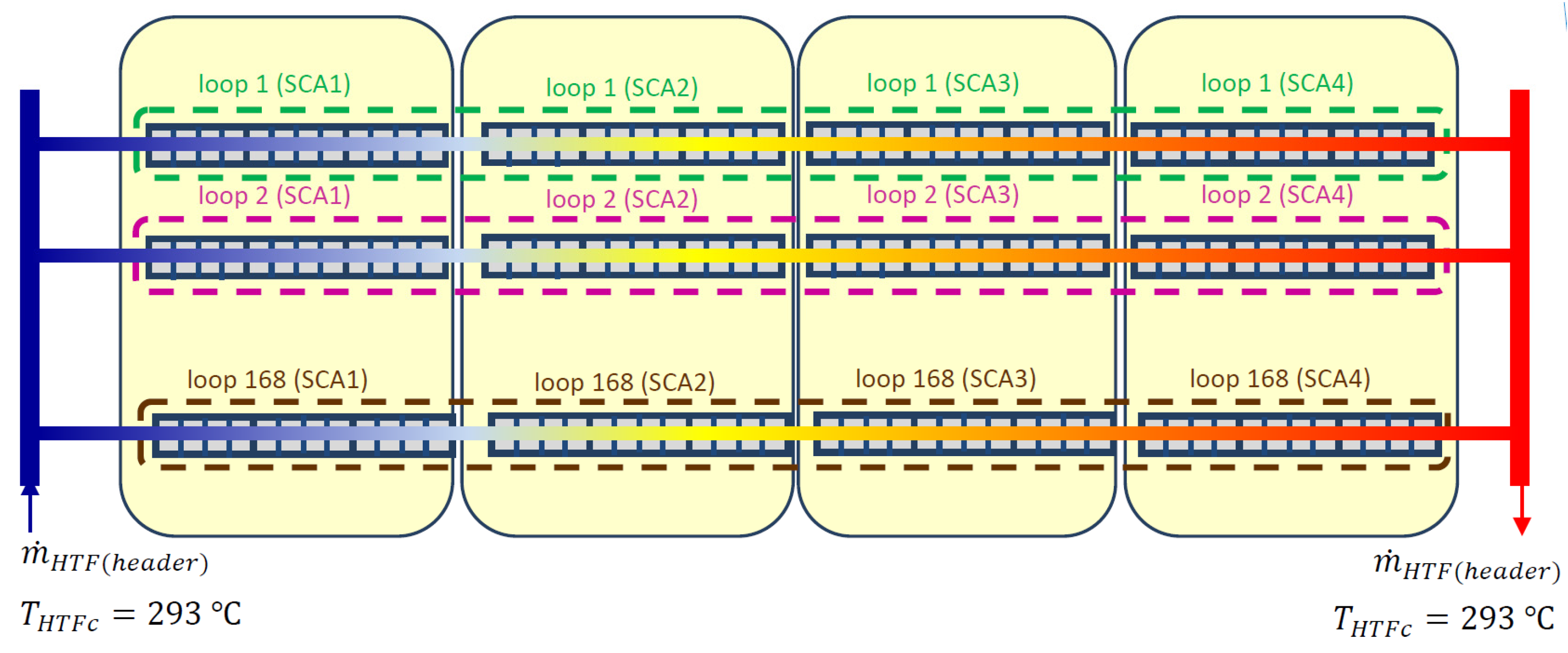
To model the HTF-heating process, some simplifications of the SF must be carried out, namely, the 168 loops have been modeled as four serial-connected unitary blocks. Each unitary block contains 168 parallel-connected SCAs. This configuration is shown in Figure 8.

Figure 8. Loop simplification.

Figure 8. Loop simplification.

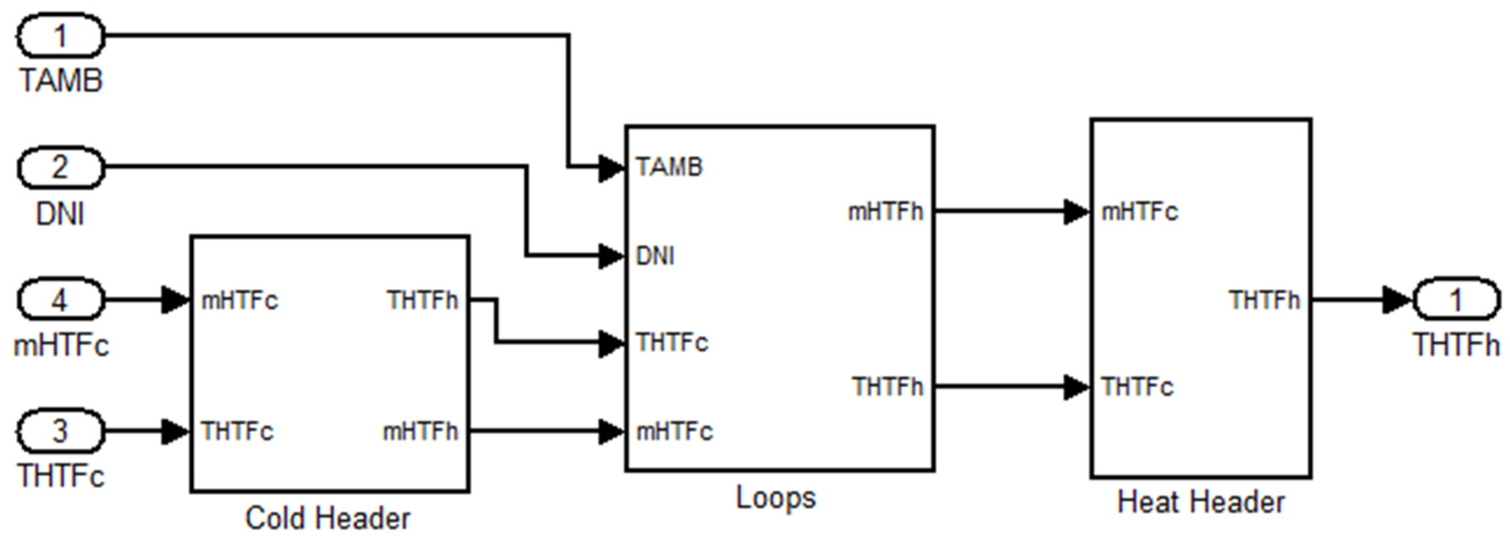
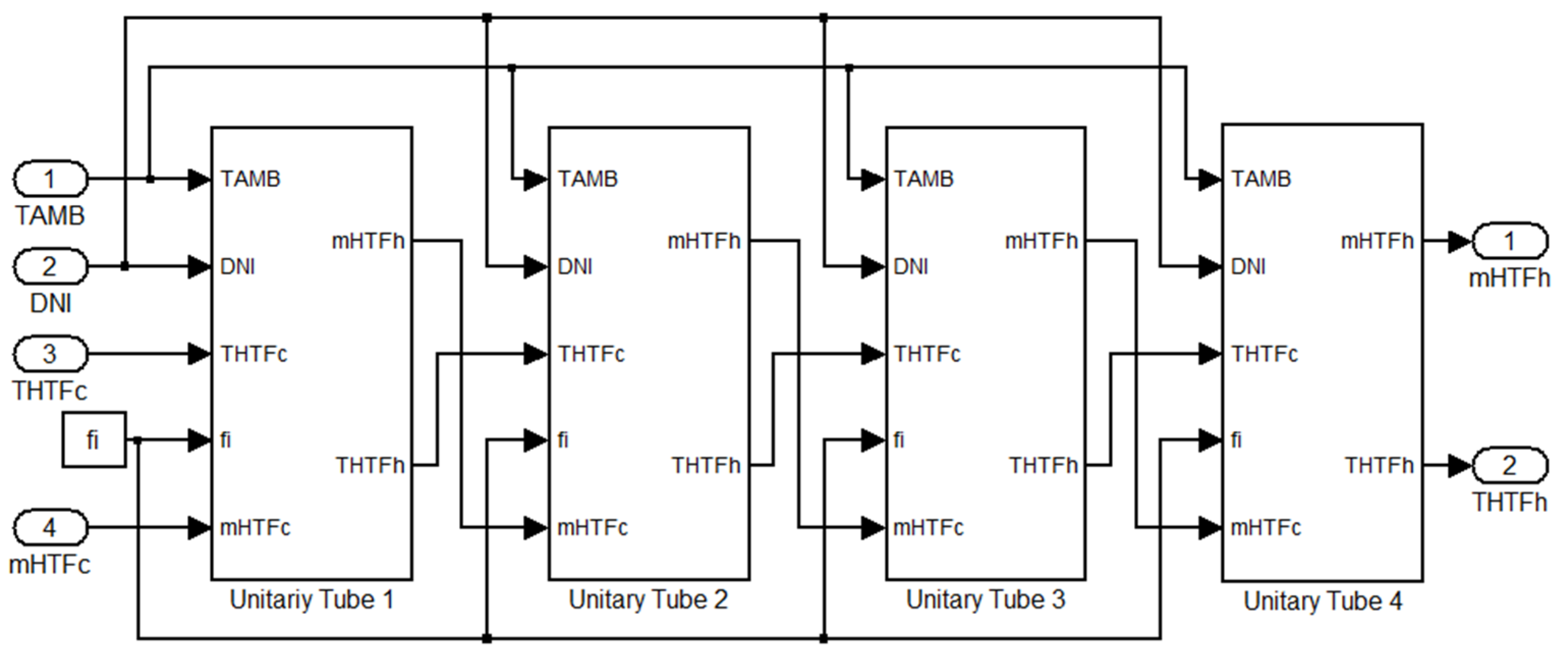
Similarly, the headers are modeled as four serial-connected blocks, each containing a quarter of the total amount of HTF. Figure 9 shows the block diagram of the SF to be used in the modeling of the HTF-heating process, and Figure 10 shows the blocks used to model the loops described above.

Figure 9. Solar field (SF) model.

Figure 9. Solar field (SF) model.

Figure 10. Loops model.

Figure 10. Loops model.

These Simulink blocks can be easily used for modeling larger or smaller SFs by respectively adding or removing unitary tubes.

Energy transfer from solar radiation to the fluid takes place inside the unitary tubes as well as inside the headers. For that reason, all the equations related to mass and energy conservation principles should be included in those blocks.

The conservation energy principle provides the following equations:

$${\dot{E}}_{\text{input}}={\dot{E}}_{\text{output}}$$

(1)

Energy can be transferred as work, heat and mass:

$${\dot{Q}}_{\text{in}}+{\dot{W}}_{\text{in}}+(\dot{m}·e{)}_{\text{in}}={\dot{Q}}_{\text{out}}+{\dot{W}}_{\text{out}}+(\dot{m}·e{)}_{\text{out}}$$

(2)

where $\dot{Q}$ is the absorbed or released heat, $\dot{W}$ is the work done by the HTF and e is the energy transported per unit mass of a moving fluid, whose expression is given by Equation (3):

$$e=h+\frac{1}{2}{V}^2+gz$$

(3)

Finally, assuming that in the absorber pipes kinetic and gravitational energies are negligible and that, due to the mass conservation principle in the control volume considered in the process, input and output mass flows are similar, Equation (2) is simplified as indicated in Equation (4):

$$h\left(t\right)={{\displaystyle \int }}_0^t\frac{{\dot{m}}_{\text{HTF }}·\left(h_i-h_o\right)+{\dot{Q}}_{\text{gain}}}{{\rho }_{\text{HTF}}·{\upsilon }_{\text{c}}}·\text{d}t$$

(4)

where ${\dot{Q}}_{\text{gain}}$ is the heat that the HTF absorbs from the solar radiation once all the losses due to thermal transfer from the fluid to the environment have been taken into account.

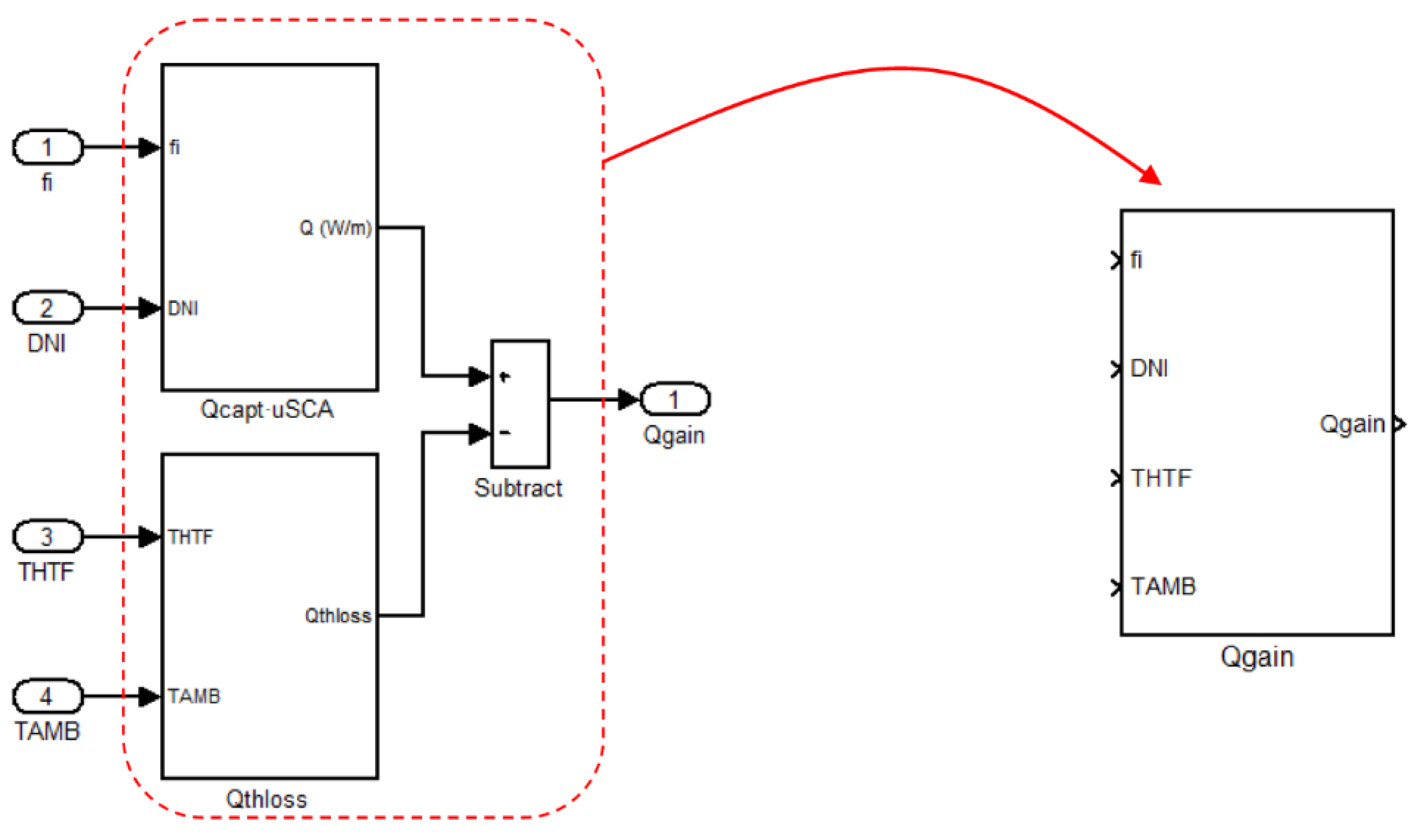
The net heat transferred from the HTF to other subsystems of the solar plant is the result of the total heat absorbed by the fluid minus the thermal losses due to radiation, convection and conduction from the fluid to the air around it.

The heat absorbed by the fluid depends on geometric, optical and thermal factors. Firstly, not all the solar radiation that reaches the mirrors (${\dot{Q}}_{\text{capt}}$) is reflected over the absorber tubes and then absorbed by the fluid, due to phenomena such as shadows, angle of incidence far from the optimal 90°, dirty mirrors, non-optimal reflectivity and transmissivity, etc. This results in the heat that reaches the fluid being reduced by the efficiency of the SCA (${\mathsf{\eta }}_{\text{SCA}}$). Additionally, of all the heat reaching the fluid, some is lost in unwanted thermal transfers (${\dot{Q}}_{\text{thloss}}$):

$${\dot{Q}}_{\text{gain}}={\dot{Q}}_{\text{capt}}·{\mathsf{\eta }}_{\text{SCA}}-{\dot{Q}}_{\text{thloss}}$$

(5)

All these phenomena have been modeled in a Simulink block (Figure 11) called ${\dot{Q}}_{\text{gain}}$.

Figure 11. Simulink block model to calculate ${\dot{Q}}_{\text{gain}}$.

Figure 11. Simulink block model to calculate ${\dot{Q}}_{\text{gain}}$.

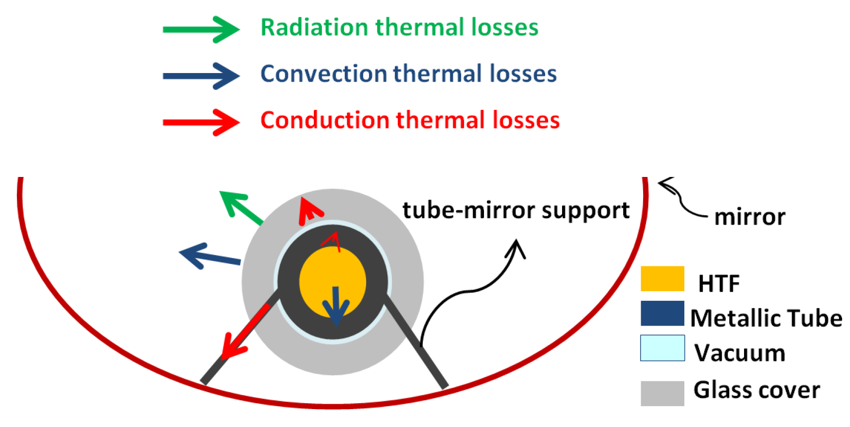
Figure 12 shows all the thermal exchanges involved in the different parts of the SCE (mirrors, absorber tube, HTF) with the environment. Some of those losses are negligible when compared to others [15,16,17]. This is the case of conduction and convection losses between the outer wall of the metallic tube and the inner wall of the glass cover (thanks to the vacuum created between them), or of conduction thermal losses produced in the walls of the tubes to mention a few.

Figure 12. Thermal exchanges between solar collector elements (SCE) and surround ambient.

Figure 12. Thermal exchanges between solar collector elements (SCE) and surround ambient.

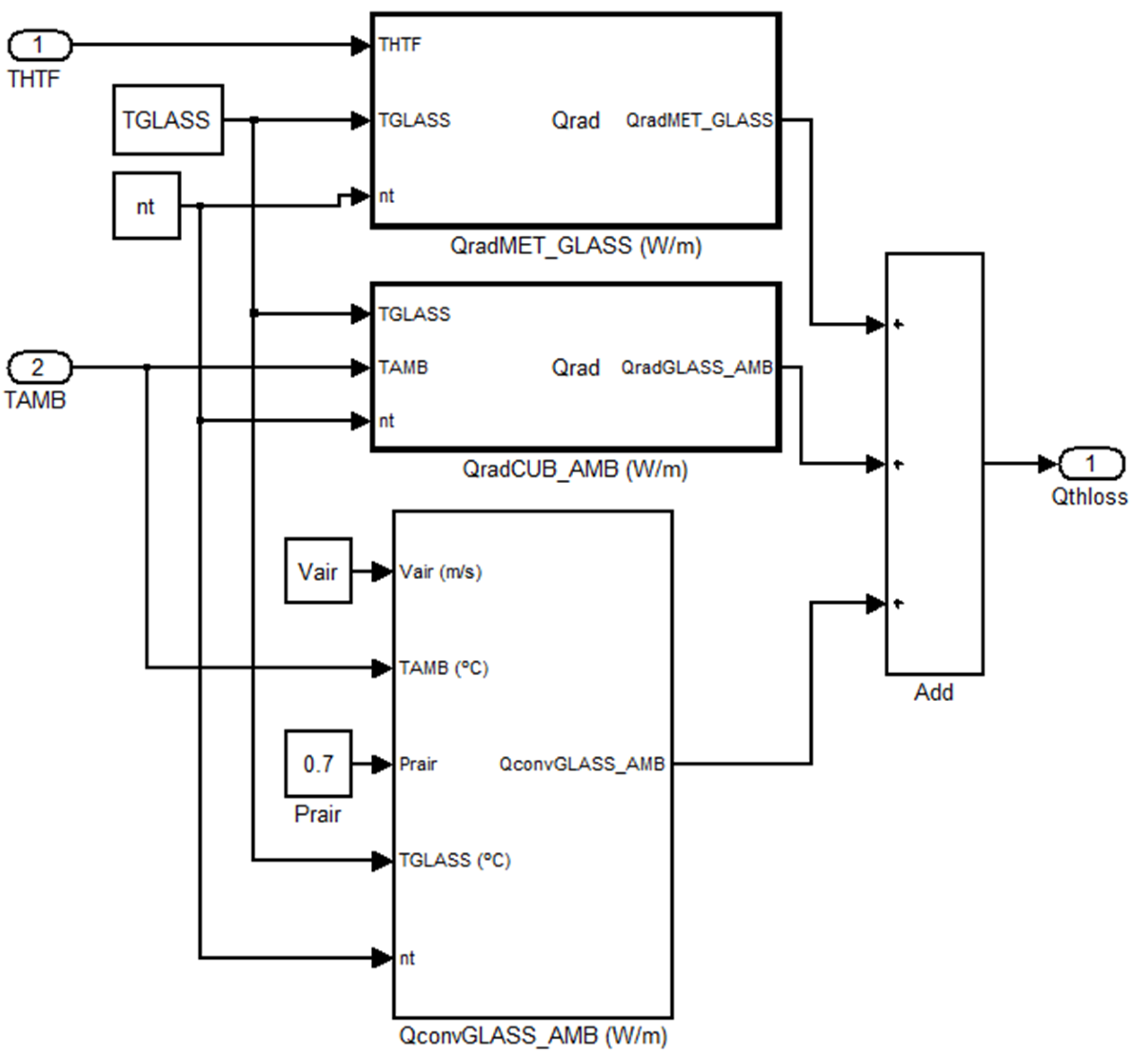
Figure 13 shows the Simulink blocks used to model all those thermal losses, which are included in the ${\dot{Q}}_{\text{thloss}}$ block of Figure 11.

Several equations are included in these blocks:

$${\dot{Q}}_{\text{radGLASS}-\text{AMB}}={\mathsf{\epsilon }}_{\text{CUB}}·\mathsf{\sigma }·A{e}_{\text{GLASS}}·\left(T_{\text{GLASS}}^4-T_{\text{AMB}}^4\right)$$

(6)

where ${\dot{Q}}_{\text{radGLASS}-\text{AMB}}$ represents the radiation thermal losses per meter (W/m) from the outer wall of the absorber pipe glass cover to the environment, ${\mathsf{\epsilon }}_{\text{GLASS}}$ is the emissivity coefficient of the external surface of the glass cover, $\mathsf{\sigma }$ is the Stefan-Boltzmann constant (W/m²·C⁴), $A{e}_{\text{GLASS}}$ is the external surface of the absorber pipe glass cover per unit length (m²/m) and $T_{\text{GLASS}}$ and $T_{\text{AMB}}$ are, respectively, the glass cover and the ambient temperatures (°C):

$${\dot{Q}}_{\text{convGLASS}-\text{AMB}}=h_{\text{GLASS}-\text{AMB}}·A{e}_{\text{GLASS}}·\left(T_{\text{GLASS}}-T_{\text{AMB}}\right)$$

(7)

where ${\dot{Q}}_{\text{convGLASS}-\text{AMB}}$ represents the convection thermal losses per meter (W/m) from the outer wall of the absorber pipe glass cover to the surround ambientand $h_{\text{GLASS}-\text{AMB}}$ is the convection coefficient between the external surface of the glass cover and the surround ambient. This coefficient is highly dependent on wind speed and can be calculated as:

$$h_{\text{GLASS}-\text{AMB}}=\frac{N{u}_{\text{AMB}}}{D{e}_{\text{GLASS}}}·K_{\text{AMB}}$$

(8)

In Equation (8), $N{u}_{\text{AMB}}$ is the dimensionless Nusselt number, $D{e}_{\text{GLASS}}$ is the outer diameter of the glass cover and $K_{\text{AMB}}$ is the thermal conductivity of the air.

To calculate the Nusselt number, Hilpert equation for forced convection flow is used:

$$N{u}_{\text{AMB}}=C·R{e}^m·P{r}^{1/3}$$

(9)

where Re is the dimensionless Reynolds number and parameters, C and m depend on the value of the Reynolds number. $Pr$ is the dimensionless Prandtl number of the air, the value of which is around 0.7.

Finally, the dimensionless Reynolds number of the air over the outer wall of the glass cover is calculated from Equation (10):

$$Re=\frac{V_{\text{air}}·D{e}_{\text{GLASS}}·{\mathsf{\rho }}_{\text{air}}}{{\mathsf{\mu }}_{\text{air}}}$$

(10)

where $V_{\text{air}}, {\mathsf{\rho }}_{\text{air}}, {\mathsf{\mu }}_{\text{air}}$ are the air speed, density and dynamic viscosity respectively.

Equation (11) is used to calculate thermal radiation transference from the outer surface of the metallic pipe to the inner wall of the glass cover ${\dot{Q}}_{\text{radMET}-\text{CUB}}$:

$${\dot{Q}}_{\text{radMET}-\text{GLASS}}=\frac{\mathsf{\sigma }·A{e}_{\text{MET}}·(T_{\text{MET}}^4-T_{\text{GLASS}}^4)}{\frac{1}{{\mathsf{\epsilon }}_{\text{MET}}}+\frac{1-{\mathsf{\epsilon }}_{\text{GLASS}}}{{\mathsf{\epsilon }}_{\text{GLASS}}}·\left(\frac{D{e}_{\text{MET}}}{D{i}_{\text{GLASS}}}\right)}$$

(11)

where $A{e}_{\text{MET}}$ is the external surface of the metalic pipe per unit length (m²/m) and $T_{\text{MET}}$ and $T_{\text{GLASS}}$ are, respectively, the metallic pipe and the glass cover temperatures (°C).

Figure 13. Thermal losses blocks.

Figure 13. Thermal losses blocks.

Once all the blocks have been defined and all the equations have been included, the dynamic model of the HTF heating process is obtained. Figure 14 shows the Simulink diagram that includes all the blocks and equations described above. Inside that block there are the four unitary tubes that contain the time-dependent Equation (4) as well as the block ${\dot{Q}}_{\text{gain}}$ described in Figure 11. In this way, the fluid temperature varies along the path as do all the temperature-dependent variables (enthalpy, fluid density, etc.).

Figure 14. HTF heating process.

Figure 14. HTF heating process.

3. Experimental Section

To validate the already developed model, the control strategy usually applied in thermoelectric solar plants was implemented. Due to the complexity of a PTC solar plant and the amount of subsystems included in it, there are many controllers to regulate different outputs: mirrors position (in order to have the lowest possible optical losses), temperature and flow rate in the TES system (in order to have as much storage as possible during the molten salt charge process and the highest energy transference to the fluid in the discharging mode [1]) and so on. To cope with all this, solar plants must have a distributed control system (DCS) [21] that receives field signals (such as ambient temperature, HTF temperature, incident angle, the DNI, etc.) and sends them to the appropriate controller, which generates the adequate actions in each case.

The control of the HTF heating is typically performed in either of two different ways. Some plants have a semiautomatic proportional-integral-derivative (PID) regulator that relies on an operator observing the output variables of the process, mainly the HTF temperature, and changing the mass flow input set point to make this output temperature be constant despite the perturbations. Once the mass flow input set point has been fixed by the operator, internal PID regulators will operate the pumps to achieve that set point. This semiautomatic method has two drawbacks: in addition to its accuracy depending on the operator’s experience, it is carried out by steps. Figure 15 shows a diagram of the regulator.

Figure 15. Semiautomatic control of the HTF-heating process.

Figure 15. Semiautomatic control of the HTF-heating process.

More modern plants have substituted the operator by an external PID regulator in such a way that this new controller is the one that determines the HTF mass flow to achieve as a result of a comparison between the real temperature of the HTF at the output of the SF (THTFh) and the set point of the fluid temperature at the output of the SF, previously fixed (SPTHTFh). Figure 16 shows the PID automatic control.

Figure 16. Proportional-integral-derivative (PID) automatic control of the HTF-heating process.

Figure 16. Proportional-integral-derivative (PID) automatic control of the HTF-heating process.

Figure 17 shows how the dynamic model of the heating process was linked to a model of a PID regulator using also Matlab and Simulink. Different perturbations where introduced in the input variables (Tamb, DNI and THTFc) and the performance of the system was analyzed.

Figure 17. MatLab-Simulink model of the PID control for the HTF-heating process.

Figure 17. MatLab-Simulink model of the PID control for the HTF-heating process.

Figure 18 shows the response of the process to a sharp step perturbation in the DNI. This sort of perturbations may occur, for example, when multiple clouds suddenly disappear.

Figure 18. PID controller response to a sharp step in direct solar irradiation (DNI).

Figure 18. PID controller response to a sharp step in direct solar irradiation (DNI).

It is possible to see that the behavior of the PID when there is a sharp variation in the solar radiation is far from optimal, and a very high temperature can be reached, which would result in faster fluid degradation. Besides, the settling time is also high so any intent to reduce the high peak, will give rise to an even slower settling time. The slow response to a rapid and sharp change in an input variable as the DNI can be explained by the amount of time the oil stays in the SF, which gives rise to thermal inertia. One of the effects of this inertia is transport delay; a variation of temperature at the inlet of the pipe is not reflected at the output until sometime later. The other effect of thermal inertia is similar to a filtering. At a constant flow rate, a step of radiation produces a variation in the temperature at the loop output that looks like a pure delay stage with respect to the variation of radiation.

In the collectors that gather and mix the oil from the loops, the HTF of each loop has a different delay depending on their distance to the power block (also called power island), which is normally located in the center or north of the SF. The overall effect is that a step in the solar radiation results in a delay plus an additional filtering effect in such a way that the global response to that step is a pure delay followed by a second-order overdamped response.

Once the steady state has been established, the average error between the set point and the real temperature is below 1 °C.

The model was also subjected to values of the input variables extracted from an actual plant called ”La Africana” situated in Cordoba, Spain. These values were taken in different years and seasons: September 2010, April 2011 and July 2013 and they were extracted from the DCS. The response of the model developed in this paper, to those input variables can be seen in Figure 19, Figure 20 and Figure 21.

In these figures, horizontal axis represents the time in seconds and the vertical axis shows the true representation of the absolute values of the different variables.

Figure 19 shows that, when variations in the input variables are not sharp, the PID response does not involve high peak temperatures. Table 3 shows the error average value (μ) and the error standard deviation (σ) calculated for all the values obtained during 5 h.

Table 3. Numerical results of simulation with PID (September 2010).

Control Strategy	Input Values	$e=SPTHT{F}_h-THT{F}_h$
		μ	σ
Proportional-integral-derivative (PID) controller	September 2010	−1.92	3.27

Table 3. Numerical results of simulation with PID (September 2010).

Control Strategy	Input Values	$e=SPTHT{F}_h-THT{F}_h$
		μ	σ
Proportional-integral-derivative (PID) controller	September 2010	−1.92	3.27

Figure 19. PID controller response to September 2010 values.

Figure 19. PID controller response to September 2010 values.

Figure 20. PID controller response to April 2011 values.

Figure 20. PID controller response to April 2011 values.

Figure 21. PID controller response to July 2013 values.

Figure 21. PID controller response to July 2013 values.

When solar radiation falls below a certain value, however, the PID controller is not able to provide rapid response and temperature deviates greatly from its set point, as can be seen in Figure 20. This is also confirmed by the value of the standard deviation in Table 4.

Table 4. Numerical results of simulation with PID (April 2011).

Control Strategy	Input Values	$e=SPTHT{F}_h-THT{F}_h$
		μ	σ
PID controller	April 2011	6.35	15.11

Table 4. Numerical results of simulation with PID (April 2011).

Control Strategy	Input Values	$e=SPTHT{F}_h-THT{F}_h$
		μ	σ
PID controller	April 2011	6.35	15.11

If the set of values corresponding to a DNI under 500 W/m² are removed, the error and standard deviation values are shown in Table 5.

Table 5. Numerical results of simulation with PID (April 2011).

Control Strategy	Input Values	$e=SPTHT{F}_h-THT{F}_h$
		μ	σ
PID controller	April 2011	−3.20	12.04

Table 5. Numerical results of simulation with PID (April 2011).

Control Strategy	Input Values	$e=SPTHT{F}_h-THT{F}_h$
		μ	σ
PID controller	April 2011	−3.20	12.04

Figure 21 shows the PID response when there are quick and sharp changes in the solar direct normal irradiation. Even though the PID succeeds in following these variations, the oscillation is high and the standard deviation is large, as indicated in Table 6.

Table 6. Numerical results of simulation with PID (July 2013).

Control Strategy	Input Values	$e=SPTHT{F}_h-THT{F}_h$
		μ	σ
PID controller	July 2013	−4.06	25.90

Table 6. Numerical results of simulation with PID (July 2013).

Control Strategy	Input Values	$e=SPTHT{F}_h-THT{F}_h$
		μ	σ
PID controller	July 2013	−4.06	25.90

Looking at the PID response for different values of the input variables (some of which have been obtained from an actual thermal power plant), it can be shown that this controller has an adequate behavior when those input variables do not vary suddenly. However, it has a very slow response to quick variations; therefore this control method should be improved if the global efficiency of these plants has to be optimized.

The goal of this paper, however, is not determining what the best control strategy is, but rather defining a model of the SF that can be later used to optimize such strategies. In this regard, it must be said the results obtained with the model presented match those measured in the actual plant under similar conditions.

4. Conclusions

A dynamic model of the HTF heating process as it flows through the SF has been developed. The use of Simulink has allowed a model of the process to be obtained that is very visual and easy to follow. Besides, since it has been built from the simplest blocks to the more complicated ones, it can also be used to model the fluid heating process of other solar plants with different sizes by just adding or removing unitary tubes (see Figure 10).

Some of the fluid properties such as density, thermal conductivity, specific heat, etc. have been included as temperature dependent equations that can be easily changed so that the model can be also used in solar plants where the HTF is not synthetic oil (as in the case considered) but water steam, molten-salt, etc.

Looking at Figure 18, Figure 19, Figure 20 and Figure 21 it is possible to see that, even though a PID controller might be suitable when there are no rapid changes in environment conditions, its response is slow when a sharp change is produced. The developed model is able to identify this situation and can therefore be used to test other algorithms of control, such as predictive ones, adaptative, and so on, to optimize the behavior of the HTF temperature controller without interfering in the operation of the plant, i.e. using just simulations. Once the regulator has been selected, it can be implemented in the real plant.

References

1. Peón Menéndez, R.; Martínez, J.A.; Prieto, M.J.; Barcia, L.Á.; Martín Sánchez, J.M. A Novel Modeling of Molten-Salt Heat Storage Systems in Thermal Solar Power Plants. Energies 2014, 7, 6721–6740. [Google Scholar] [CrossRef]
2. Barlev, D.; Vidu, R.; Stroeve, P. Innovation in concentrated solar power. Sol. Energy Mater. Sol. Cells 2011, 95, 2703–2725. [Google Scholar] [CrossRef]
3. Kuravi, S.; Trahan, J.; Goswami, D.Y.; Rahman, M.M.; Stefanakos, E.K. Thermal energy storage technologies and systems for concentrating solar power plants. Prog. Energy Combust. Sci. 2013, 39, 285–319. [Google Scholar] [CrossRef]
4. Kenisarin, M.M. High-temperature phase change materials for thermal energy storage. Renew. Sustain. Energy Rev. 2010, 14, 955–970. [Google Scholar] [CrossRef]
5. Gil, A.; Medrano, M.; Martorell, I.; Lazaro, A.; Dolado, P.; Zalba, B.; Cabeza, L.F. State of the art on high temperature thermal energy storage for power generation. Part 1—Concepts, materials and modellization. Renew. Sustain. Energy Rev. 2010, 14, 31–55. [Google Scholar] [CrossRef]
6. Medrano, M.; Gil, A.; Martorell, I.; Potau, X.; Cabeza, L.F. State of the art on high-temperature thermal energy storage for power generation. Part 2—Case studies. Renew. Sustain. Energy Rev. 2010, 14, 56–72. [Google Scholar] [CrossRef]
7. Montes, M.J.; Abánades, A.; Martínez-Val, J.M. Thermofluidynamic Model and Comparative Analysis of Parabolic Trough Collectors Using Oil, Water/Steam, or Molten Salt as Heat Transfer Fluids. J. Sol. Energy Eng. 2010, 132. [Google Scholar] [CrossRef]
8. Montes, M.J.; Abanades, A.; Martinez-Val, J.M.; Valdes, M. Solar multiple optimization for a solar-only thermal power plant, using oil as heat transfer fluid in the parabolic trough collectors. Sol. Energy 2009, 83, 2165–2176. [Google Scholar] [CrossRef] [Green Version]
9. Lopez-Gonzalez, D.; Valverde, J.L.; Sanchez, P.; Sanchez-Silva, L. Characterization of different heat transfer fluids and degradation study by using a pilot plant device operating at real conditions. Energy 2013, 54, 240–250. [Google Scholar] [CrossRef]
10. Feldhoff, J.F.; Schimtz, K.; Eck, M.; Schnatbaum-Laumann, L.; Ortiz-Vives, F.; Laing, D.; Schulte-Fischedick, J. Comparative system analysis of direct steam generation and synthetic oil parabolic trough power plants with integrated thermal storage. Sol. Energy 2012, 86, 520–530. [Google Scholar] [CrossRef]
11. Haddad, Z.; Abid, C.; Oztop, H.F.; Mataoui, A. A review on how the researchers prepare their nanofluids. Int. J. Therm. Sci. 2014, 76, 168–189. [Google Scholar] [CrossRef]
12. Flamant, G.; Gauthier, D.; Benoit, H.; Sans, J.L.; Boissiere, B.; Ansart, R.; Hemati, M. A new heat transfer fluid for concentrating solar systems: Particle flow in tubes. Energy Procedia 2014, 49, 617–626. [Google Scholar] [CrossRef]
13. Ghadimi, A.; Saidur, R.; Metselaar, H.S.C. A review of nanofluid stability properties and characterization in stationary conditions. Int. J. Heat Mass Transf. 2011, 54, 4051–4068. [Google Scholar] [CrossRef]
14. Alguacil, M.; Prieto, C.; Rodriguez, A.; Lohr, J. Direct steam generation in parabolic trough collectors. Energy Procedia 2014, 49, 21–29. [Google Scholar] [CrossRef]
15. Osório, T.; Carvalho, M.J. Testing of solar thermal collectors under transient conditions. Energy Procedia 2012, 30, 1344–1353. [Google Scholar]
16. Thorsen, S.; Blair, N.; Mitchell, J.A.; Beckman, W.A. Automatic Control of a 30 MWe SEGS VI parabolic trough plant. Sol. Energy 2004, 76, 187–193. [Google Scholar]
17. Roldán, M.; Cañadas, I.; Casas, J.L.; Zarza, E. Thermal analysis and design of a solar prototype for high-temperature processes. Int. J. Heat Mass Transf. 2013, 56, 309–318. [Google Scholar] [CrossRef]
18. Burkholder, F.; Kutscher, C. Heat Loss Testing of Schott’s 2008 PTR70 Parabolic Trough Receiver; National Renewable Energy Laboratory: Golden, CO, USA, 2009.
19. Roldán, M.; Valenzuela, L.; Zarza, E. Thermal analysis of solar receiver pipes with superheated steam. Appl. Energy 2013, 103, 73–84. [Google Scholar] [CrossRef]
20. Eck, M.; Feldhoff, J.F.; Uhlig, R. Thermal Modelling and Simulation of Parabolic Trough Receiver Tubes. In Proceedings of the 4th International Conference of Energy Sustainability, Phoenix, AZ, USA, 17–22 May 2010; pp. 659–666.
21. Bong-Kuk, L.; Yong-Hak, S. The integrated monitoring and control system for the combined cycle power plant. In Proceedings of the International Conference on Control, Automation and Systems, Seoul, Korea, 14–17 October 2008; pp. 1479–1483.