3.1. Change-Time-Priority-List Method
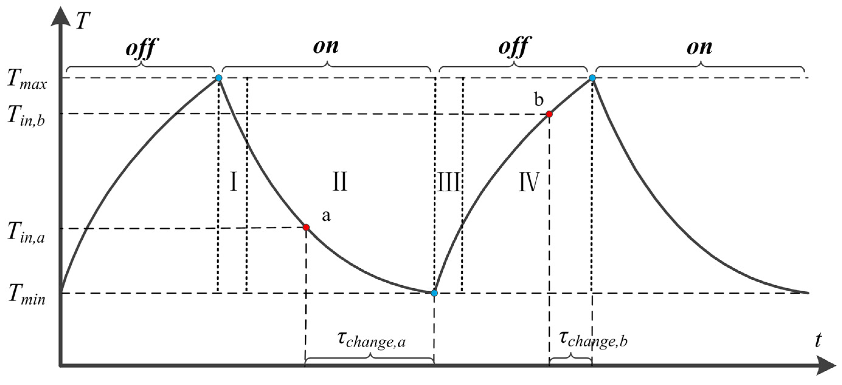
For the change-time-priority-list method, ACs are divided into two groups based on their on/off state. ACs in the “on” group are arranged in ascending order according to their change time from on to off. If it is required to reduce load, ACs with shorter change time take precedence to be turned off. Similarly, ACs in the “off” group are arranged in ascending order according to their change time from off to on. If it is required to increase load, ACs with shorter change time take precedence to be turned on. Point a in
Figure 3 denotes an AC in the “on” group; while point b refers to an AC in the “off” group, with their corresponding indoor temperature being
Tin,a and
Tin,b. The change time from on to off of AC on point a is τ
change,a, and the change time from off to on of AC on point b is τ
change,b. Limits of indoor temperature are [
Tmin,
Tmax]. With all these variables taken into Equations (8) and (9), we can obtain:
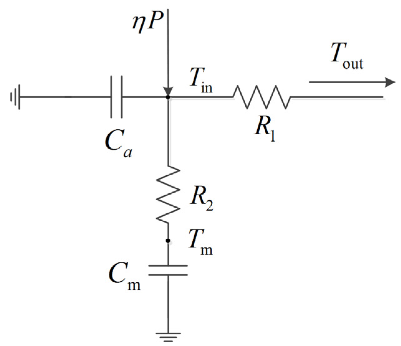
Figure 3.
Thermal dynamics of an air conditioner (AC) unit.
Figure 3.
Thermal dynamics of an air conditioner (AC) unit.
ACs with shorter change time are close to natural state change point (the blue point in
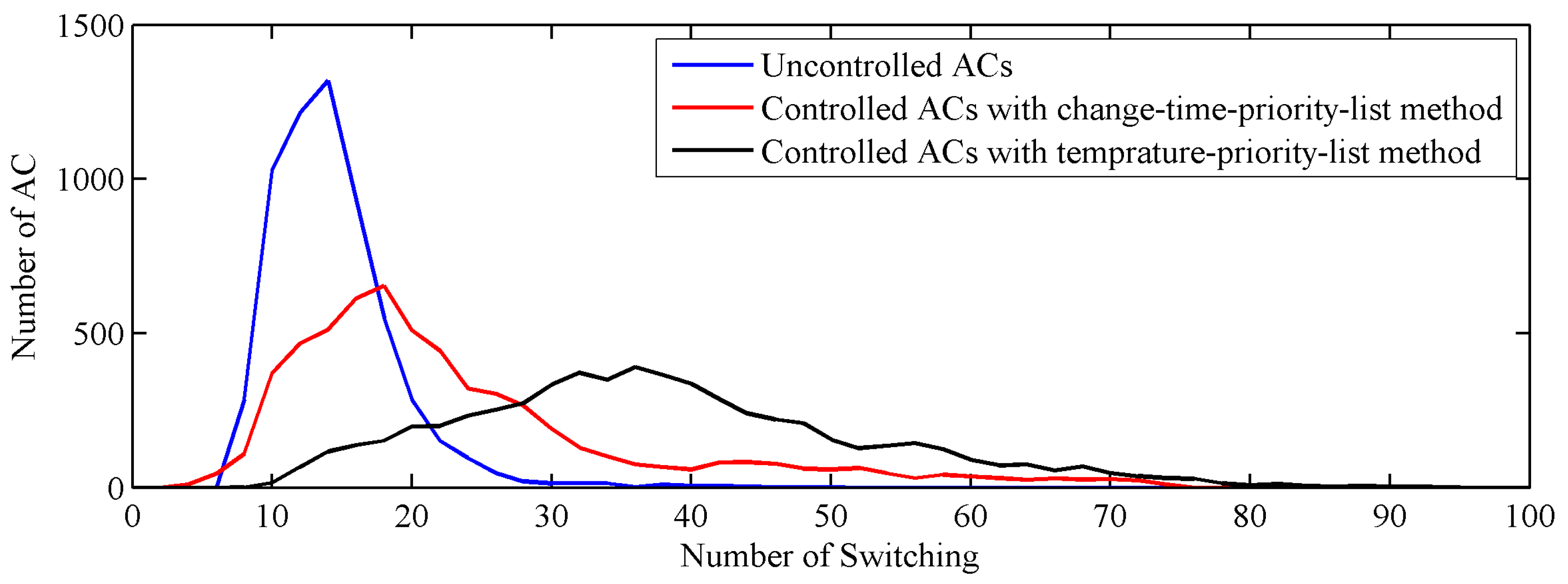
Figure 3); therefore, this paper takes priority to control ACs with shorter change time in order to minimize interference with consumers. The change-time-priority-list method takes advantage over temperature-priority-list method proposed in [
27]. Firstly, temperature-priority-list method only makes sense when the temperature setpoint of each AC is the same, while the change-time-priority-list method makes it possible for consumers to select temperature setpoint freely. Secondly, change-time-priority-list method is more widely applicable. Though, for a population of homogeneous ACs, the two methods are identical, and the change-time-priority-list method performs much better than temperature-priority-list method for a population of heterogeneous ACs, which will be discussed in detail in the case study.
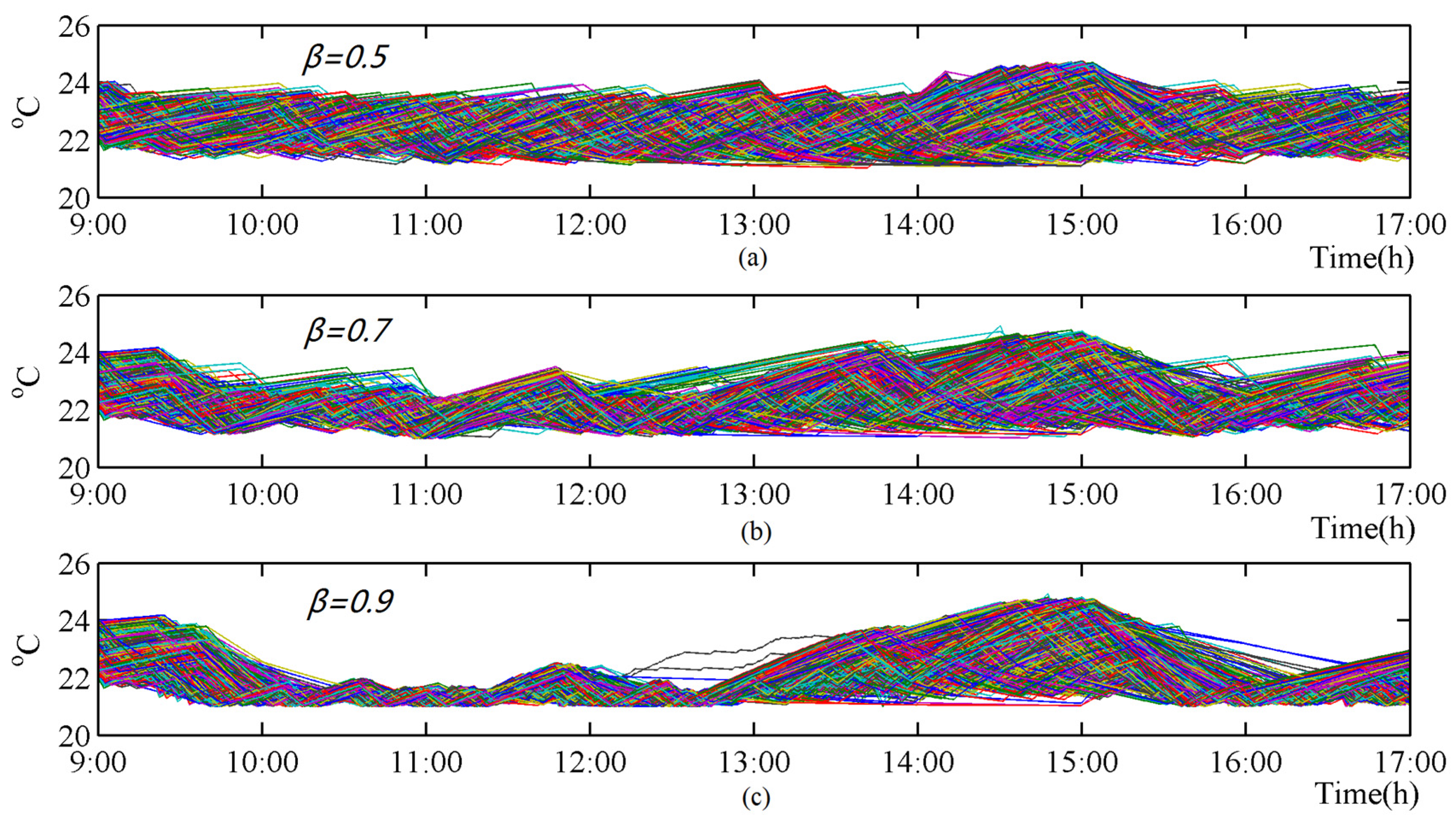
Four regions in
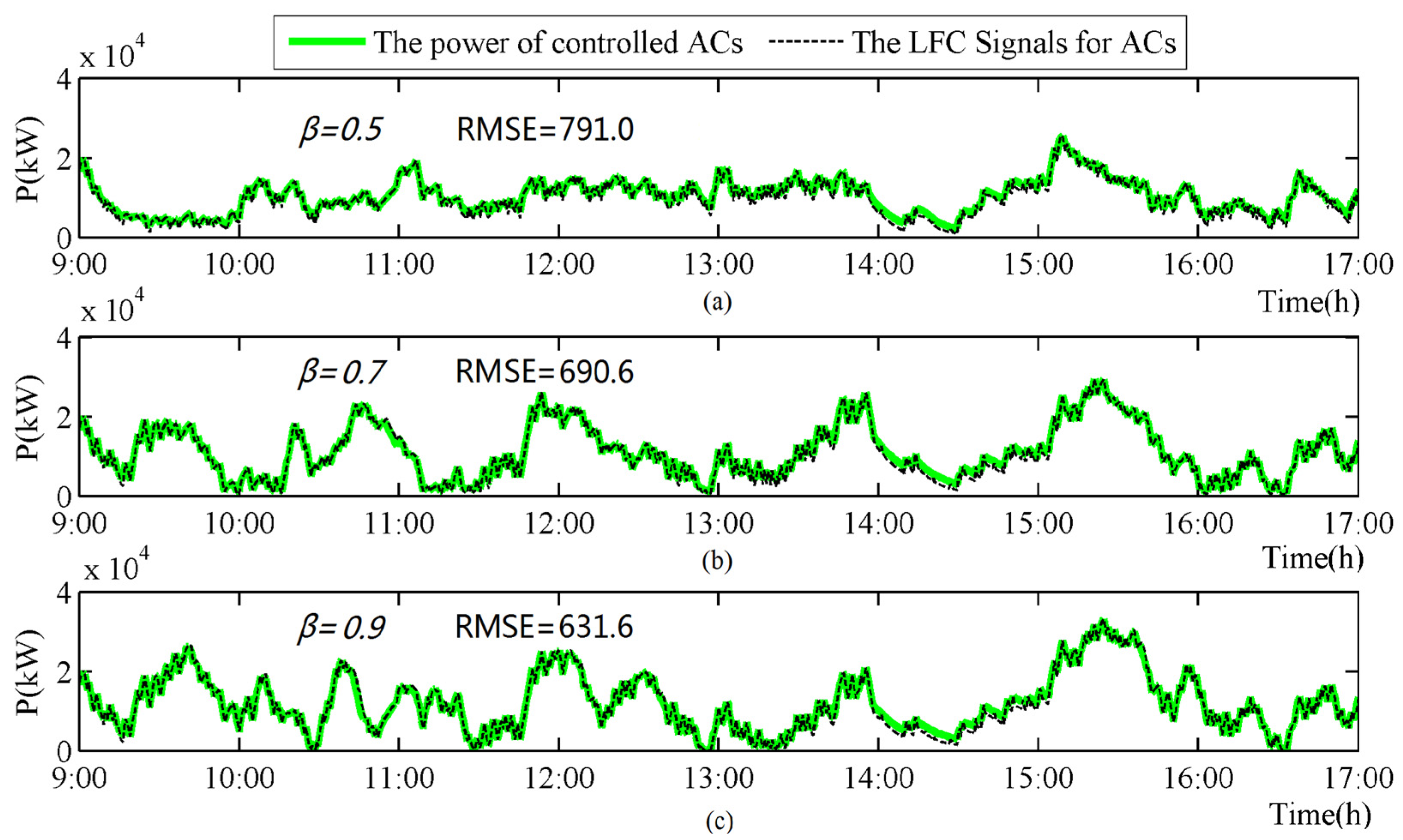
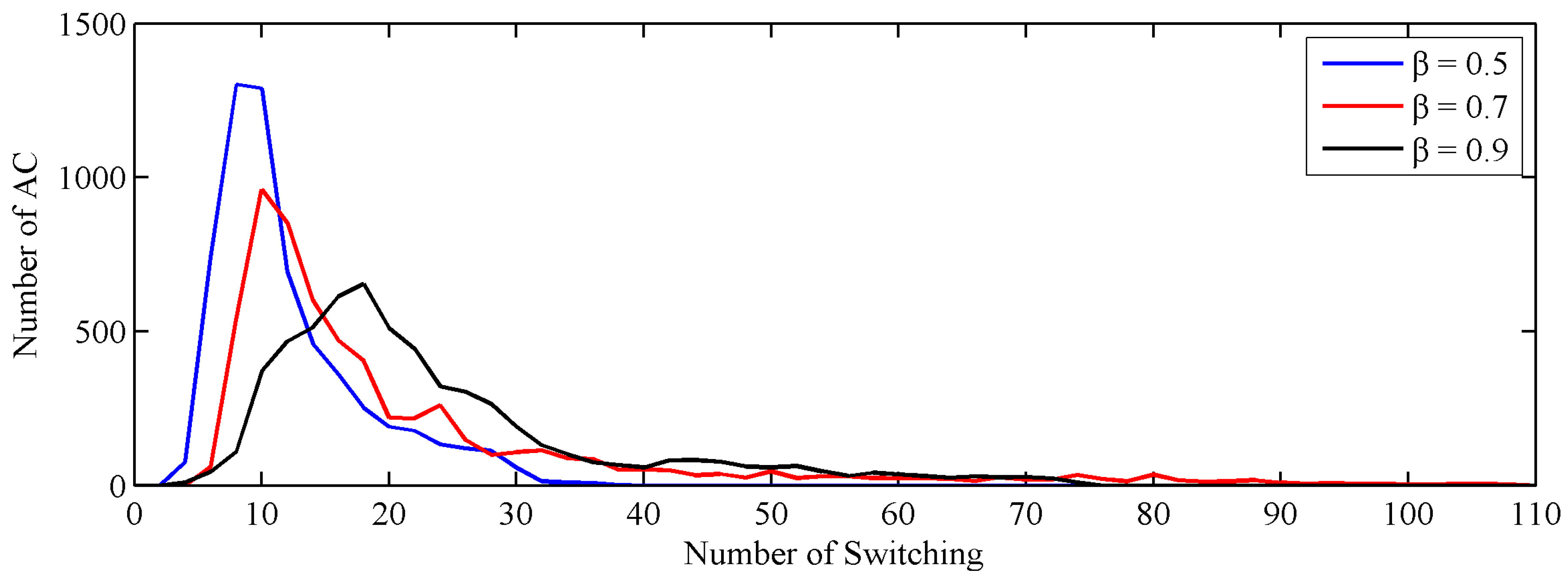
Figure 3 are implemented to tell ACs which regions are suitable for control. ACs in Region I are not suitable for control because these ACs, which are just turned on, would be automatically switched on again soon after manually turned off, while ACs in Region II are appropriate for control. ACs in Region III are uncontrollable on account of their short-time closure, while ACs in Region IV are appropriate for control. Parameter β is introduced to tell which region the
ith AC belongs to:
3.2. Combining with the Traditional Load Frequency Control
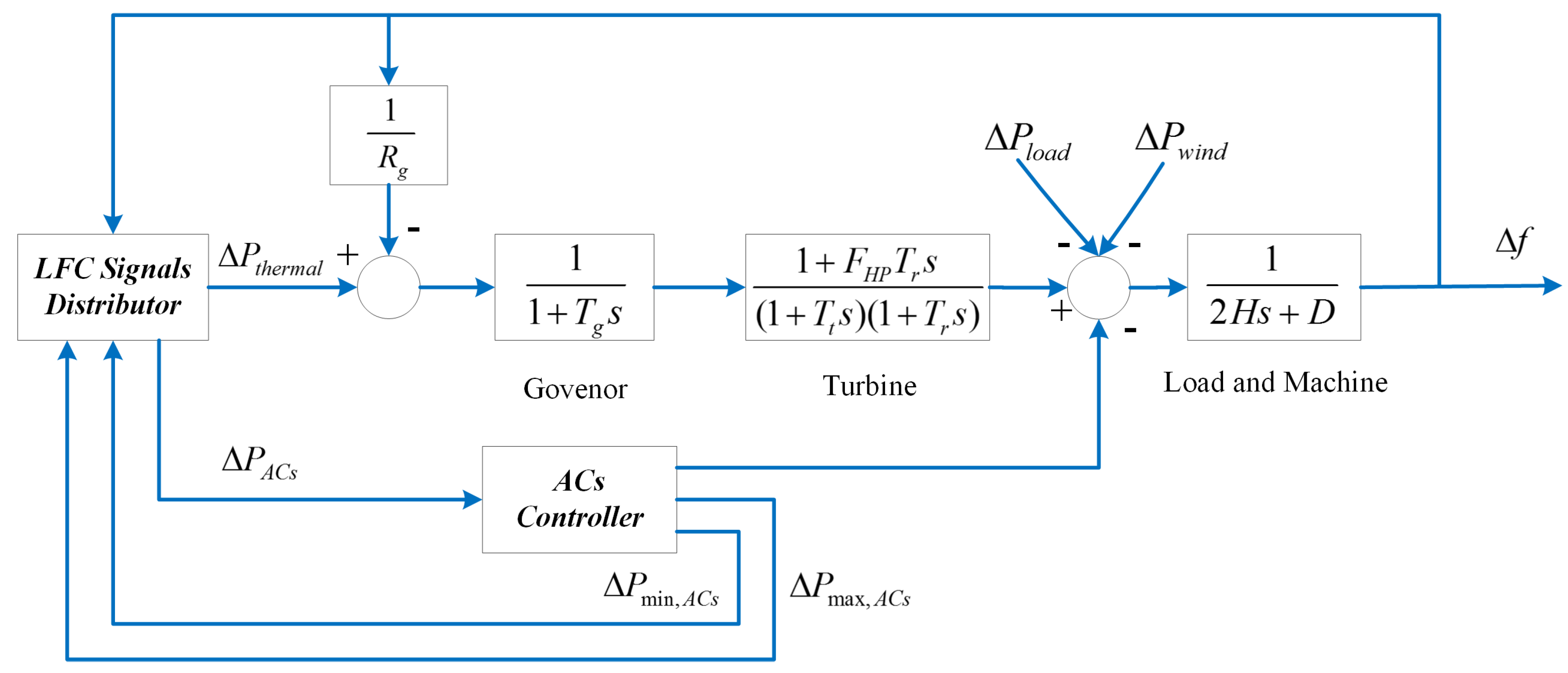
The frequency response model of the power system is shown in
Figure 4. Supplement LFC provided by aggregated ACs is integrated with conventional LFC, which is the model of the simulation in this paper. The detailed parameters of this model are summarized in
Table 1.
Figure 4.
Simulation system for combining supplement LFC with the traditional LFC.
Figure 4.
Simulation system for combining supplement LFC with the traditional LFC.
Table 1.
Parameters of simulation system.
Table 1.
Parameters of simulation system.
| Parameters | Description | Unit |
|---|
| Laplace operator | - |
| Deviation of system frequency | Hz |
| Speed governor time constant | s |
| Power fraction of the high pressure turbine section | p.u. |
| Reheat time constant | s |
| Turbine time constant | s |
| Inertia constant of generators and motors | p.u.·s |
| Load-damping constant | p.u./Hz |
| Speed droop | Hz/p.u. |
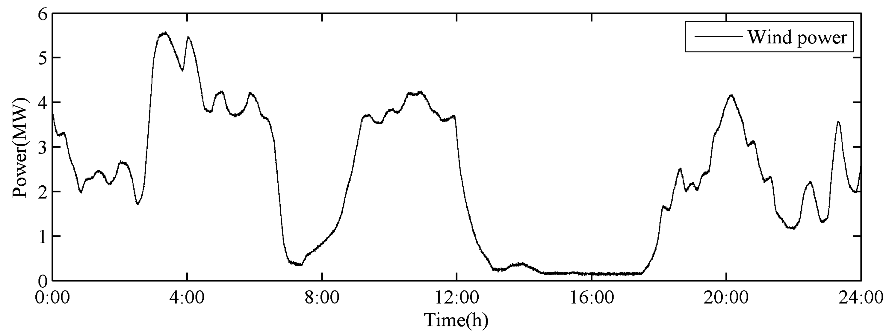
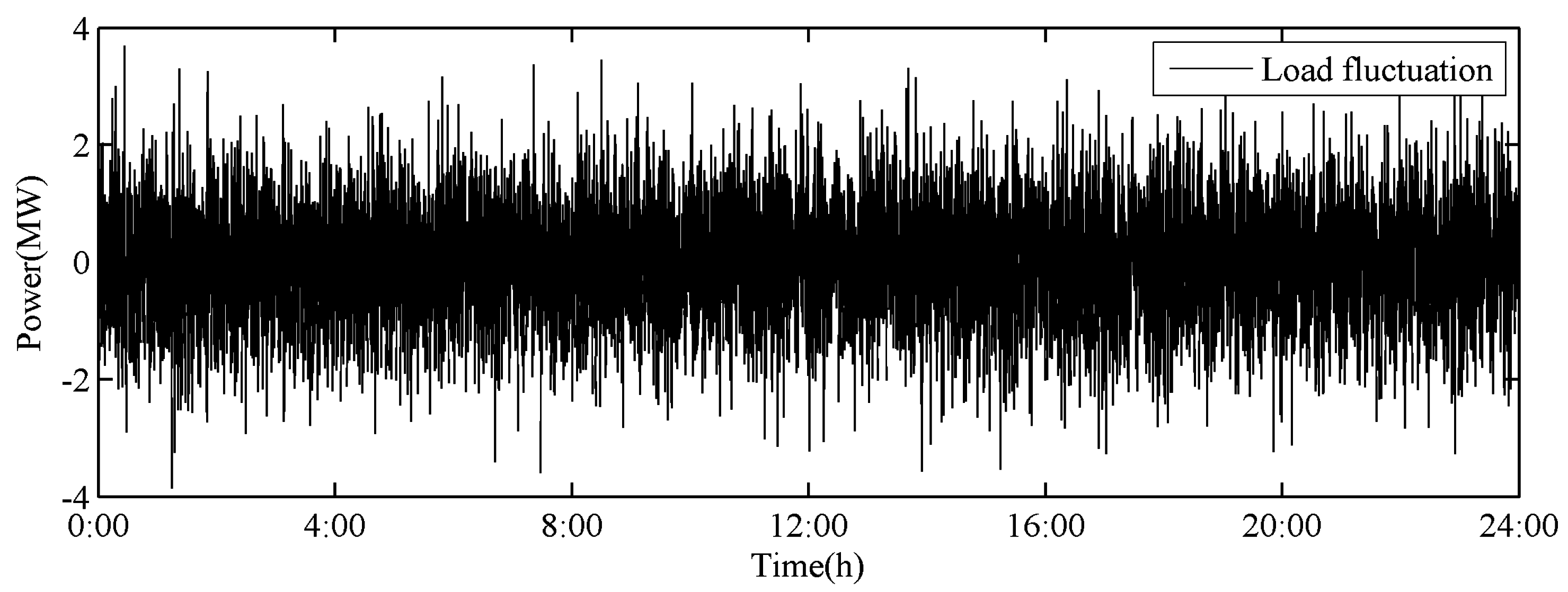
| Load fluctuation | MW |
| Wind power output fluctuation | MW |
| LFC signals for thermal plant | MW |
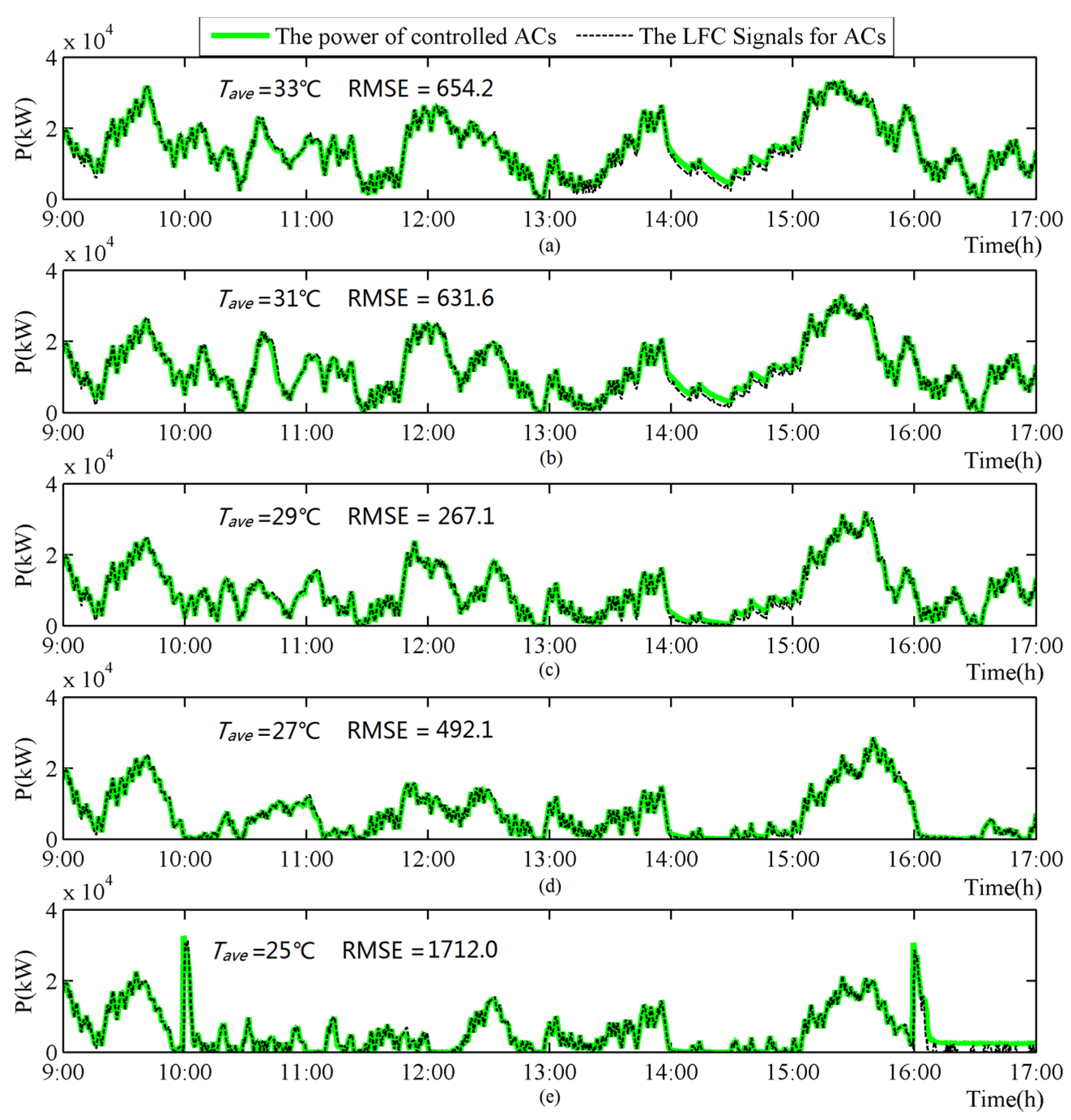
| LFC signals for aggregated ACs | MW |
| The upper limit of ACs’ power changes | MW |
| The lower limit of ACs’ power change | MW |
The simulation system is composed of two parts: one is the frequency response model of the power system including governor block, turbine block, load and machine block and 1/
Rg block (see [
5,
6]); the other are the two blocks proposed in this paper—LFC signal distributor and AC controller.
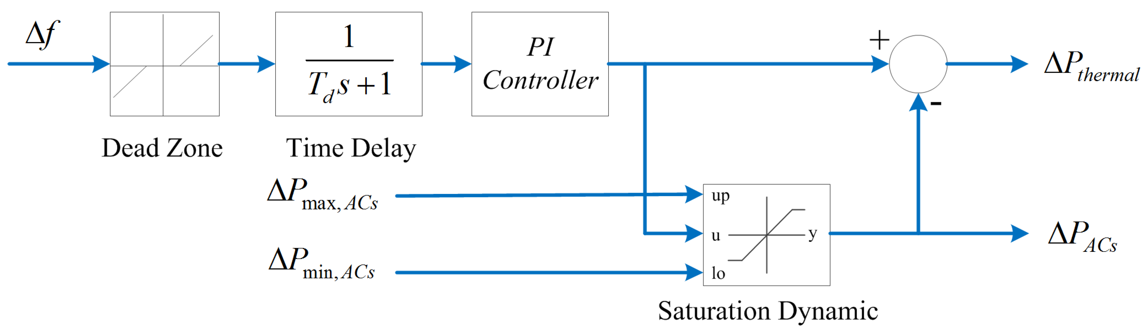
LFC signals distributor is implemented to calculate the LFC signal of thermal plant and aggregated ACs (
Figure 5). Signal distribution is realized through saturation dynamic block and
sent back from ACs controller.
Figure 5.
Block diagram of the LFC signal distributor. Proportional-integral: PI.
Figure 5.
Block diagram of the LFC signal distributor. Proportional-integral: PI.
AC controller block is realized through the MATLAB-function. The ACs under change-time-priority-list method are prioritized in ascending order based on their change time, i.e., ACs with shorter change time would be at the top of the list to be controlled. At the same time, the impact of AC natural on/off state change on the control results is also taken into consideration. Specific procedures are as follows.
Step 1: The change time of individual AC
and the aggregated load of
N ACs without control on time
t are calculated by formula in Equations (10) or (11), in which
denotes the estimated AC on/off state on time
t and
Ri,
Ci,
Pi denote AC characteristic parameters.
Step 2: Assume Δ
t is the time step of AC control. For ACs meet
≤ Δ
t and
s = 1, their change time is less than time step; therefore, these ACs would automatically be switched from on to off in this period. Assume the set of these ACs is
, the total power is:
Step 3: For ACs meet
≤ Δ
t and
s = 0, their change time is also less than time step; therefore, these ACs would automatically be switched from off to on in this period. Assume the set of these ACs is
, the total power is:
Step 4: Assume the frequency fluctuation signal on time
t is
Δft and the limits of aggregated AC load is Δ
and Δ
, Δ
and Δ
could be calculated by LFC distributor block. Note that positive Δ
indicates that the output of generators needs to be increased. While positive Δ
indicates that aggregators are needed to turn off ACs so as to decrease load.
- ●
If Δ > ( − ), go to Step 5;
- ●
If Δ < ( − ), go to Step 6;
- ●
If Δ = ( − ), go to Step 7.
Step 5: It is required to reduce load in this step. We can use Equation (13) to tell which AC belongs to Region II. Apart from the
ACs in Step 2, there are
−
controllable ACs in total. Work out the change-time-priority-list of these ACs and select several ACs from the top of the list. Assume the set of these selected ACs is
, which should make Equation (19) hold:
Step 6: It is required to increase load in this step. ACs in region IV are determined through Equation (15): apart from the
ACs in Step 3, there are
−
ACs in total. Work out the change-time-priority-list of these ACs and select several from the top of the list as
, we can get:
Step 7: No more operations are needed except for ACs belong to set and . Turn off ACs in and turn on ACs in .
Step 8: Calculate the controlled AC power on time
t:
Step 9: This step aims to estimate the value of several variables on time
t +1. According to the control result in Steps 5–7,
could be deduced by
and the indoor temperature on time
t + 1 could be calculated by Equations (1) and (2). Equations (10)–(15) could be used to locate ACs in each region. Similarly, the upper and lower limits of aggregated power on time
t + 1 could be estimated by:
It could be concluded that the upper limit of aggregated load could be obtained by turning on aggregated ACs in region IV, while the lower limit of aggregated load could be obtained by turning off aggregated ACs in region II.
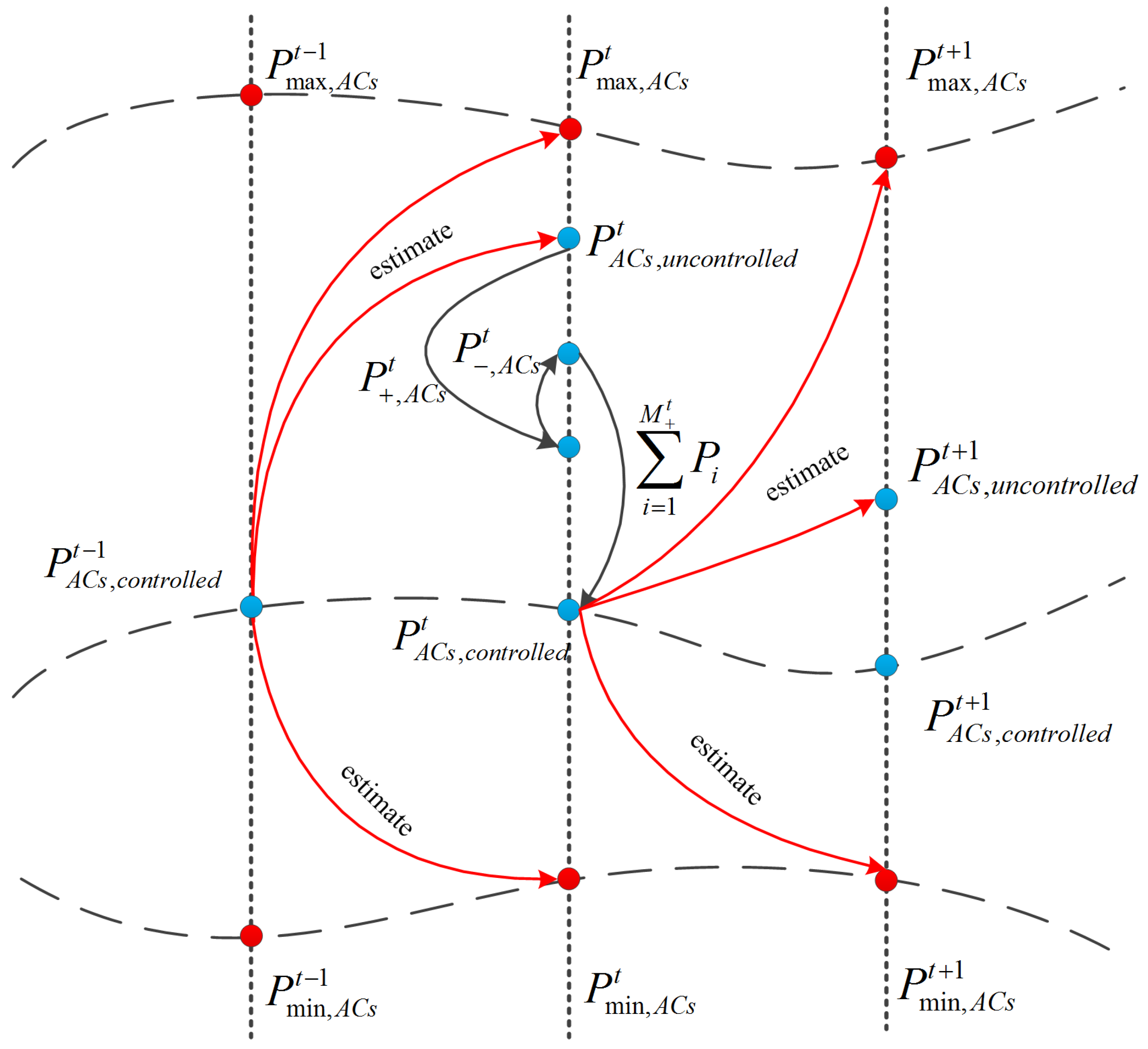
Figure 6 demonstrates the process from Steps 1 to 9. Aggregators need to estimate the uncontrolled aggregated AC load
the limits of aggregated AC load
and
on time
t − 1.
and
is determined by Steps 2 and 3. Steps 4–7 aim to select ACs to be controlled and calculate the controlled aggregated AC load
. According to this value, uncontrolled aggregated AC load on time
t + 1
and the limits of aggregated AC loadon time
t + 1
and
could be estimated.
Figure 6.
Schematic diagram of the process from Steps 1 to 9.
Figure 6.
Schematic diagram of the process from Steps 1 to 9.


