A Simplified Simulation Model for Predicting Radiative Transfer in Long Street Canyons under High Solar Radiation Conditions

Abstract

Modeling solar radiation in street canyons is crucial to understanding the solar availability of building façades. This article describes the implementation of a simulation routine, developed in the Matlab^® computer language, which is aimed at predicting solar access for building façades located in dense urban conglomerates comprising deep long street canyons, under high solar radiation conditions, typical in southern countries of Europe. Methodology is primarily based on the configuration factor theory, also aided by computer simulation, which enables to assess the interplay between the surfaces that compose the so-called street canyon. The results of the theoretical model have been cross-checked and verified by on-site measurements in two real case studies, two streets in Cadiz and Seville. The simplified simulation reproduces the shape of the curve for on-site measured values and weighted errors for the whole model do not surpass 10%, with a maximum of 9.32% and a mean values of 6.31%. As a result, a simplified predictive model that takes into account direct, diffuse and reflected solar radiation from the surfaces that enclose the canyon, has been devised. The authors consider that this research provides further improvement, as well as a handy alternative approach, to usual methods used for the calculation of available solar radiation in urban canyons, such as the Sky View Factor or the ray tracing.

1. Introduction

In the urban context, solar availability has a significant influence in building performance [1]. As several authors agree, an adequate management of solar energy in the urban layout can lead to a reduction in the energy consumption of buildings [2,3].

In the past recent years, efforts have been mainly focused on devising scientific tools aimed at improving energy performance in buildings [4], as well as their lighting conditions [5]. Most of the simulation procedures conceive buildings as isolated entities, encircled somehow by contour conditions. Although this hypothesis takes into account the surroundings, it either neglects or excessively simplifies their real interaction with the object of study. As they assume that elements of the surrounding urban tissue, that is, surfaces that compose nearby structures, are just an aseptic framework, these elements not directly interact with the building, far beyond obstructing solar radiation.

Buildings located within street canyons represent a specific case in this context. To clarify this point, we refer to the term street canyon as aligned buildings along both sides of a narrow street [6]. Street canyon severely influences daylighting availability in the adjacent buildings. Therefore, it is not feasible to assume open field conditions as a valid input. Due to this specific situation, researchers have devised specific tools for a better understanding of daylight illuminance [7], heat transfer [8] energy demand [9] and human comfort [10] in street canyons, making a simplification of the real object of study to a certain extent. Most of these tools match their results with RADIANCE^® or SOLENE^® software and they neglect the comparison with on-site measurements. Besides, it is commonly considered the ratio of the street canyon, height (H) and width (W), with the example H/W = 1. Therefore, narrower canyons typical of compact urban areas are not considered. A very illustrative example of that are several cities in the Mediterranean Arch with Arabian reminiscences, in which streets shape protect urban façades from the solar radiation excess, distinctive in that sunny climates.

Thus, further research is needed to advance in the understanding of the radiative transfer and the complex interchange of radiant energy between buildings envelopes, not only urban canyons but specifically in deep urban canyons [11], which comprise a H/W ratio over 2; moreover, validation of the method with real measurements should be highly advisable.

To accomplish this task, the proposed self-developed calculation model, created in Matlab^® programming language, aimed at predicting solar radiation availability and therefore design conditions deep street canyons, focusing special attention on the phenomenon of mutual reflections between planes. The calculation model has its very theoretical basis on the configuration factors theory [12], a geometrical concept widely used in other scientific fields like thermotechnics, which have proved to be very advantageous, in terms of calculation time and precision of results. This method, scarcely used in architecture [13] due to the difficult accuracy to determine complex surfaces, is used for the authors in emblematic buildings around the world at indoor conditions through approximation of main geometries [14]. In this research, an outdoor approach is undertaken by means of a simplified simulation model, which provides a new slant to radiative transfer in deep canyons. The calculation model is intended to present an alternative to Sky View Factors [15] or ray tracing methods; in addition, it is intended to be used in early stages of design or for an overview analysis on extant canyon façades or for predicting radiation levels in planned urban developments, applying this approach to the concept of “building envelope”.

2. Objectives and Methodology

The main objective of this research is to establish a rapid and efficient predictive model for assessing solar radiation availability on building façades located within street canyons, finding a balance between simplification of the real model and accuracy of the results. Secondary objectives, derived from the main objective, can be stated as follows:

-

Validate the accuracy and reliability of the proposed theoretical calculation model trough cross-check against on-site measurements.

-

Using the model to clarify the effect of the street canyons over the solar availability of the façades that compose it.

The proposed methodology, in order to achieve these objectives, comprises theoretical work, making use of computer simulation programs, and also fieldwork, in order to cross-check the obtained results. All steps are summed up in the following flowchart (Figure 1).

Figure 1. Decision flowchart.

Figure 1. Decision flowchart.

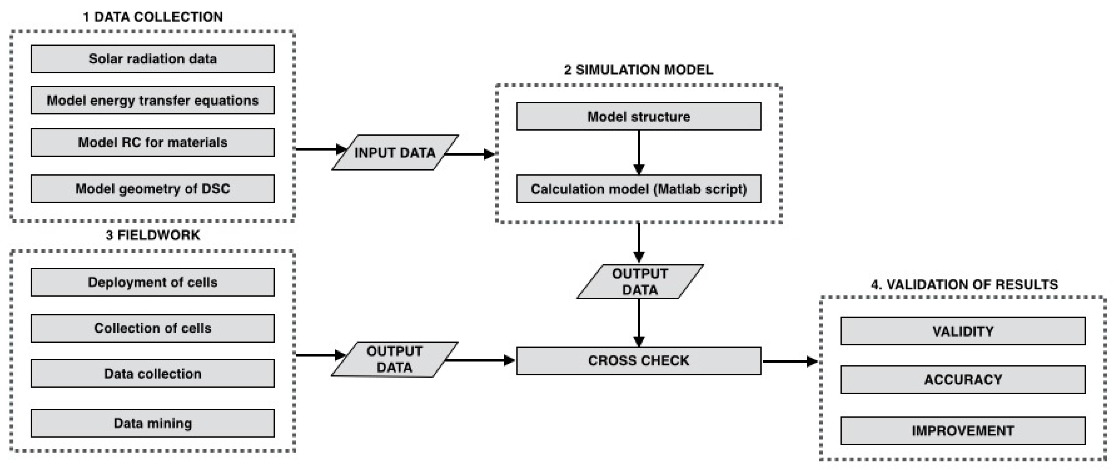
2.1. Data Collection

Different databases and sources are consulted to obtain the necessary amount of data needed in the simulation model.

• Solar radiation data is obtained from probabilistic models [16,17], which considers the probability for each type of sky (clear, partially cloudy and overcast), solar height and azimuth, and solar radiation for each main orientation (North, South, East, West, Horizontal), decomposing it into direct and diffuse component.
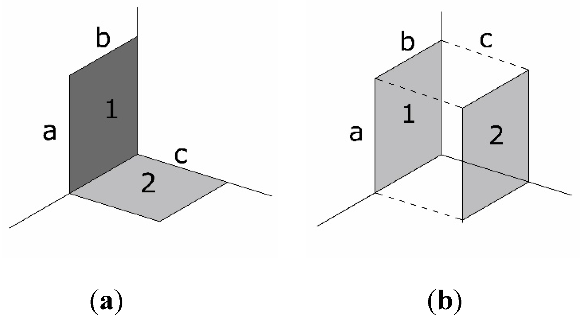
• Energy transfer equations. The fundamentals of the calculation model are based on the theory of configuration factors, in which the authors have made some contributions related with circular and spherical surfaces [18,19] and other curved surfaces [20]. Moreover, a wide database regarding these factors can be found at [21]; the authors have selected, from this source, the most relevant shapes in connection to the present case-study: View factors for rectangular surfaces [22,23] both parallel and perpendicular [24]. These factors allow for the calculation of the radiative transfer between different shapes [25], taking into account their sole geometric characteristics, that is, their shape and their relative position in the space [26]. In this case, canyon will be modeled as parallelepiped volumes composed of rectangular surfaces. In order to calculate the energy interchange between an emitting surface and the receiving planes, the simulation program will discretize the latter surfaces in unitary elements. Receiving planes will be discretized in element of 0.1 × 0.1 meters and a mesh grid is built for the calculation, which is done point by point after the division.
• Model reflection coefficients (RC) for materials: They can be easily obtained from any technical manual [27]. In this case, considered materials will be white paint (RC = 0.8), light paints, such as crème, yellow or grey (RC = 0.6) and asphalt (RC = 0.3); also, in order to facilitate the calculation process, some virtual surfaces, composed of air, will be considered as (RC = 0). RC are considered as a mean value for each of the surfaces; in the case that one of them is composed by more than one material, a weighted average value should be considered for each of them.
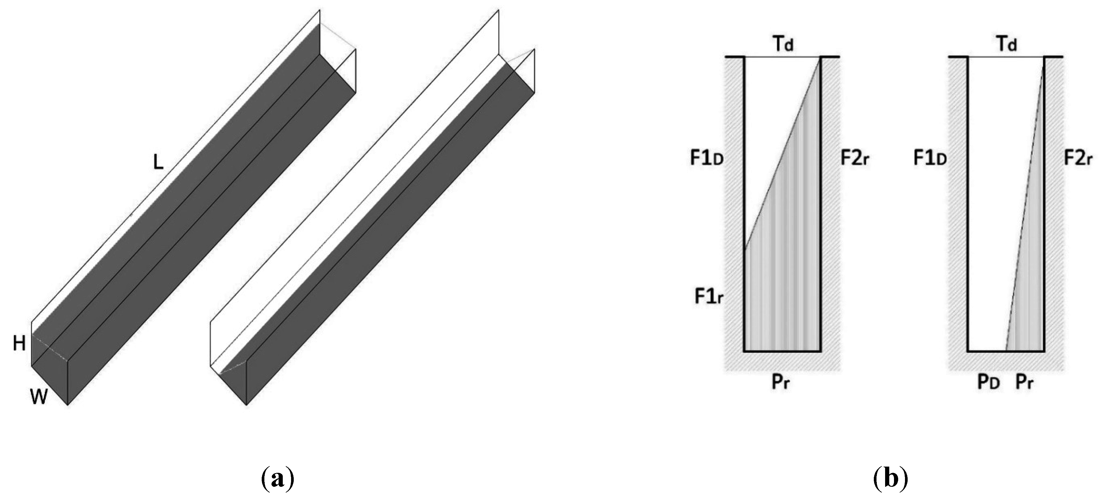
• Model geometry of the street canyon: Necessary data in this step comprises length (L), width (W) and height (H) of any given canyon.

2.2. Simulation Model

The main task at this point consists of devising a calculation model capable of admitting all data collected in step 01, process them and give, as an output, the desired information. This comprises two main subtasks:

• Devise the structure of the model, that is, which data are to be input, how the model will process them and how the results will be displayed (graphical, numerical or both).
• Insert the model and its calculation process into Matlab^® programming language. The script can be consulted in Supplementary Materials; also, additional explanations have been included in the script for a better appraisal of its functions and capabilities.

2.3. Fieldwork

In order to validate the theoretical model, a measurement campaign has been undertaken in the old quarters of the City of Cadiz [28] and Seville, located in the South of Spain (36º32′ N, 6º18′ W and 37º23′ N, 5º59′ W, respectively). They were chosen because their urban conglomerates have the necessary requirements for the present research.

Deployment of cells. Two campaigns in the case of Cadiz (Winter and Summer), and one campaign in the case of Seville (Summer) were undertaken using automatized cells HOBO^® U30 Wi-Fi Data Logger with Solar Radiation (Silicon Pyranometer) Sensor S-LIB-M003 (Measurement range: 0 to 1280 W/m²; Operating Temperature Range: −40 °C to 75 °C; Accuracy: ±10 W/m² or ±5%) in various heritage residential properties.

2.4. Data Mining

All collected data have been statistically treated using HOBOware^® and MS Excel^®. As the cells were measured over 10 days in Winter and Summer in Cádiz (10–20 January 2011; 7–17 July 2011) and over 10 days in Summer in Seville (5–15 August 2012), data mining provided with the average values that have been used to check those ones obtained from the computer simulations. Output data and cross-check of results. As two sets of output data have been obtained, that one from computer simulation and that one from on-site measurements, both of them are compared in order to check the feasibility of the proposed simulation method. Results from cross-check are focused on the following aspects:

• Validity of the method. The main question to be clarified is if the method provides with a set of useful data in order to achieve the proposed objectives, thus a critical approach about the convenience, reliability and use of resources will be taken into consideration.
• Accuracy of the method. Comparing on-site measured and simulated data, the accuracy of the method can be checked in terms of two main variables. Shape of the data curve, that is, if the model follows the pattern of the data; accuracy of numeric values, that is, if the output from the simulation routine matches those ones from the measurements. If that is not possible, the cause of the error should be found and explained, always being within an acceptable error margin.
• Improvements. Proposals in order to improve the accuracy, reliability and feasibility of the proposed simulation method will be placed into question.

3. Theoretical Basis of the Simulation Process

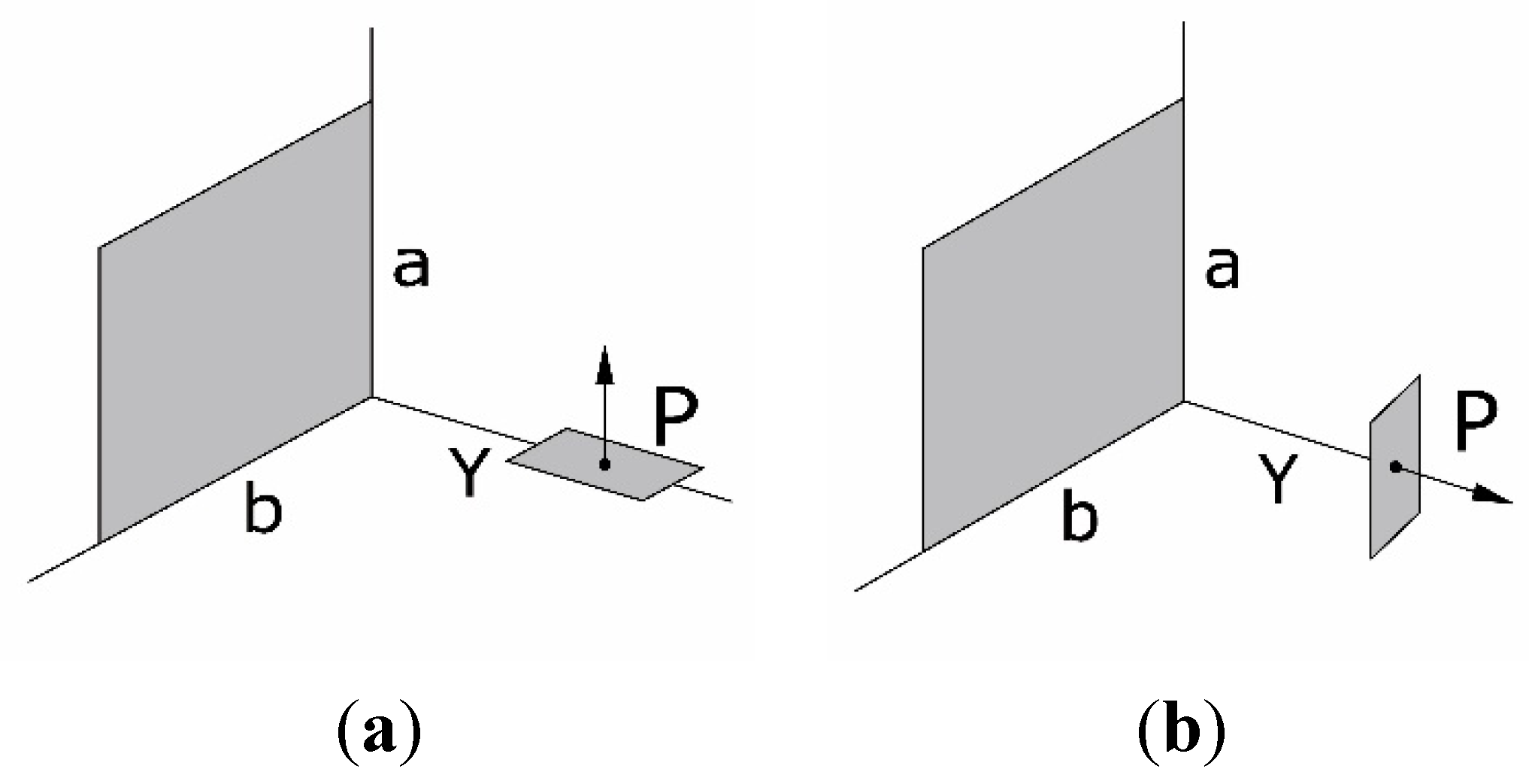
3.1. Configuration Factors and Form Factors

The fundamentals of the model is based on the theory of configuration and form factors deriving from the reciprocity principle [29], which yields the following well-known integral equation.

Equation (1) is dependent on angle, $\varnothing$, distance, r, and area, A, of the surfaces involved. Some authors have solved this equation for all sorts of curved emitters [18,19,20]. However, this research is focused on urban canyons, which can be modelled as parallelepiped volumes confined by rectangular surfaces. All of them can be calculated in a more suitable way by means of Equations (2) and (3).

$$d{\varnothing }_{1\to 2}=\left(E_{b1}-E_{b2}\right){{\displaystyle \int }}_{A_1}{{\displaystyle \int }}_{A_2}\cos {\varnothing }_1·\cos {\varnothing }_2·\frac{d{A}_1·d{A}_2 }{\pi ·r^2}$$

(1)

$$f\left(x,y\right)=\frac{E}{2}\left[\frac{\arctan b}{y}-\frac{y}{\sqrt{a^2+ y^2}}·\frac{\arctan b}{\sqrt{a^2+ y^2}}\right]$$

(2)

Equation (2) depicts the formula for radiant distribution in a point in relation to an emitting surface perpendicular to the considered point. a and b are, respectively, the horizontal and vertical dimensions of a surface having an emittance of E, and y the relative distance between the exchange points considered (Figure 2a).

$$f\left(x,y\right)=\frac{E}{2}\left[\frac{a}{\sqrt{a^2+ y^2}}·\frac{\arctan b}{\sqrt{a^2+ y^2}}+\frac{b}{\sqrt{b^2+ y^2}}·\frac{\arctan a}{\sqrt{b^2+ y^2}}\right]$$

(3)

Equation (3) depicts the radiant interchange between an emitting surface with dimensions a and b, and an emittance of E, but in this case for a point in a plane parallel to the emitting surface (Figure 2b).

Figure 2. (a) Point in relation to an emitting perpendicular surface; (b) Point in relation to an emitting parallel surface.

Figure 2. (a) Point in relation to an emitting perpendicular surface; (b) Point in relation to an emitting parallel surface.

If a point receives radiation an n number of emitting surfaces, the final configuration factor is the sum of n due to all factors. Logically, the form factor is the weighted average of all configuration factors calculated in a surface. The theory of form factor provides an additional advantage over other calculation models because of it specific algebra and their geometric basis. The additive property allows finding, by simple addition and subtraction, form factors between surfaces 1 and 2 (Figure 3a). In order to find the net exchange between these surfaces, the form factor is expressed by a dimensionless number that gives the percentage of energy, leaving surface 1 reaches to another surface 2.

The form factor between two perpendicular surfaces that share a common axis is represented in Equation (4). a is the height of the surface on the z axis, b is the distance on x axis and c is measured along the y axis (Figure 3a).

$$\begin{array}{ll}{F}_{1\to 2}=& 2bc·\text{atan}\left(\frac{b}{c}\right)+2ab·\text{atan}\left(\frac{b}{a}\right)-2b\sqrt{a^2+c^2}·\text{atan}\left(\frac{b}{\sqrt{a^2+c^2}}\right)\\ & +\frac{a^2+c^2-b^2}{2}·\text{ln}\left(a^2+b^2-c^2\right)+\frac{b^2-a^2}{2}\\ & ·\text{ln}\left(a^2+b^2\right)+\frac{b^2-c^2}{2}·\text{ln}\left(b^2·c^2\right)-\frac{a^2+c^2}{2}·\text{ln}\left(a^2+c^2\right)\\ & +a^2\text{ln}\left(a\right)-b^2\text{ln}\left(b\right)+c^2\text{ln}\left(c\right)\end{array}$$

(4)

Equation (5) depicts the form factor between two parallel surfaces separated a, c distance in the axis (Figure 3b).

$$\begin{array}{l}{F}_{1\to 2}=4b\sqrt{a^2+c^2}·\text{atan}\left(\frac{b}{\sqrt{a^2+c^2}}\right)+4a\sqrt{b^2+c^2}·\text{atan}\left(\frac{a}{\sqrt{b^2+c^2}}\right)-4bca\\ ·tan\left(\frac{b}{c}\right)-4ac-2c^2·\text{ln}\left(a^2+b^2+c^2\right)+2c^2·v\ln \left(b^2+c^2\right)+2c^2\\ ·\ln \left(a^2+c^2\right)-2c^2·\ln \left(c^2\right)\end{array}$$

(5)

Figure 3. (a) Perpendicular surfaces that share a common axis; (b) Two parallel surfaces separated a c distance.

Figure 3. (a) Perpendicular surfaces that share a common axis; (b) Two parallel surfaces separated a c distance.

3.2. Reflections

In order to establish the treatment of the reflections, Equation (6) states that the total component is the sum of the direct component and the reflected component of the 6 surfaces that compose a parallelepiped volume.

Applying this expression to the urban canyon, a parallelepiped space of six surfaces can be represent in Equation (7), where F_ij is the form factor between the surfaces i and j; ρ_i is the reflection coefficient of a given surface; E_di is the direct component of the i surface and E_ri means the reflected component from that surface.

$$E_{\text{tot}}=E_{\text{dir}}+ {\text{Σ}}_{\text{n}} ·E_{\text{ref}}$$

(6)

$$\left[\begin{array}{ccc}1& \cdots & -F_{\text{16}\rho \text{6}}\\ ⋮& \ddots & ⋮\\ -F_{\text{61}\rho \text{1}}& \cdots & 1\end{array}\right]·\left[\begin{array}{c}{E}_{\text{r1}}\\ \cdots \\ E_{\text{r6}}\end{array}\right]=\left[\begin{array}{ccc}{F}_{\text{11}\rho \text{1}}& \cdots & F_{\text{16}\rho \text{6}}\\ ⋮& \ddots & ⋮\\ F_{\text{61}\rho \text{1}}& \cdots & F_{\text{66}\rho \text{6}}\end{array}\right]·\left[\begin{array}{c}{E}_{\text{d1}}\\ \cdots \\ E_{\text{d6}}\end{array}\right]$$

(7)

4. The Simulation Model

4.1. Assumptions and Limitations

As this is a simplified model, various assumptions and limitations have been considered in order to stablish a rapid and easy-to-use calculation routine, considering minor errors, within the following boundary conditions:

-

Geometry aspect ratio. The simulation program could be used for all the height (H) divided by the width (W) proportions within the street canyon. Deep canyons, which must comprise an H/W ratio over 2 are included. The program considers symmetry or asymmetry between both sides. At this stage, the simulation tool just only considers long street canyons, which ratio length (L) divided by height (H) is over 7 [11]. That approximation was done for two main reasons: First, in order to simplify the solar hypothesis, so the direct solar radiation is parallel to the sill and the intersection between façade plane and ground plane, avoiding crossroads or other interruptions on the planes. Second, with that ratio it is possible to dismiss the slight predicted radiation from the lateral boundaries, considering the street canyon concept as an abstraction of the spatial complexity of real cities [2]. Moreover, that lateral boundaries are in most of cases difficult to predict, due to other nearby adjacent obstructions of the urban tissue. A minor error is considered because of those simplifications in central façade bands of long street canyons.

-

Surface assumptions. Terraced houses and flat façades and ground are presupposed, considering all of them as diffusive surfaces. Therefore, the radiative properties are considered as isotropic and the diffuse interreflection of the short-wave radiation obeys Lambert´s cosine law [29]. Possible discontinuities and protrusions of openings and balconies, which are produced in real streets, are dismissed in this simplified model, as well as other anisotropic surfaces.

-

Radiation. Incoming short-wave solar radiation is considered in this model, as well as the mutual diffuse interreflections. The surfaces of the canyon are considered to maintain a steady constant temperature, so long-wave radiation exchange is dismissed at this stage of approach.

4.2. Solar Radiation Hypothesis

The proposed model takes into account three main components: direct radiation as a primary source, diffuse component from the sky vault and reflected component from the surfaces composing the canyon. Street canyon is modelled as a parallelepiped of length L, width W and height H (Figure 4a). L = infinity; W and H are constant; as the concept of long street canyon is considered, the two virtual surfaces at both ends of the street are ruled out, considering a minor inaccuracy at this step. To calculate the effective radiation in each of the façades of a street canyon, it is considered that conditions vary significantly in each of the points of these surfaces. Canyon is composed of (Figure 4b): a virtual vault T_d, similar to the method of fictitious surfaces [30]; façade F1, which is the one that is impinged by direct radiation, can be divided into lighted surface F1_D and shadowed surface F1_r; street pavement P, divided again into lighted surface P_D and shadowed surface P_r; façade F2_r, which only has shadowed part. Due to solar geometry, sun can only impinges in one façade and the street pavement at once.

Figure 4. (a) Urban canyon model; (b) Lighting hypothesis within urban canyon.

Figure 4. (a) Urban canyon model; (b) Lighting hypothesis within urban canyon.

Surfaces denoted with subscript d receive diffuse radiation from the sky vault, that is, T_d. Subscript D implies receiving direct solar radiation, whether is horizontal or vertical, depending respectively on street pavement P_D (DifHR) and façades F1_D (DifVR). Subscript r indicates that this surface receives reflected component, coming from adjacent surfaces. Each one of these surfaces can be assigned with their own reflection coefficient. As several materials compose façades and pavements, a weighted mean value is adopted for each one of the whole surfaces considered.

In surfaces affected by direct sunlight, which can be F1_D and P_D, the value of radiation in open field that corresponds according to their latitude and climate is assigned (DirVR and DirHR, respectively). Once these surfaces reflect solar radiation, its radiant distribution is diffuse, point to point calculated by the method of configuration factors. Surface T_d emits with the intensity of diffuse radiation from the sky vault, producing also a diffuse distribution.

Surfaces denoted with the subscript r do not receive direct radiation from the sky, neither direct nor diffuse. Their value is assigned from the emitting surface T_d, multiplied by the correspondent form factor. Here a small simplification is made, as the form factor is the mean of all configuration factors in the limits of the given surface. However, error tolerance has demonstrated to be admissible taking this hypothesis.

In the case of overcast sky conditions or diffuse radiation in all the surfaces, the virtual surface T_d emits with the intensity of diffuse radiation from the sky vault and is multiplied by the form factor of the other surfaces that compound the street canyon (F1_r, P_r, F2_r).

Once all radiation values, geometric data and reflections coefficients have been assigned, they are introduced in the reflection matrix, Equation (8), that is embedded in the calculation script.

$$\left[\begin{array}{ccc}1& \cdots & -F_{\text{Td}\to \text{F1D}\rho \text{Td}}\\ ⋮& \ddots & ⋮\\ -F_{\text{F1D}\to \text{Td}\rho \text{F1D}}& \cdots & 1\end{array}\right]·\left[\begin{array}{c}{E}_{\text{rTd}}\\ \cdots \\ E_{\text{rF1D}}\end{array}\right]=\left[\begin{array}{ccc}{F}_{\text{Td}\to \text{Td}\rho \text{Td}}& \cdots & F_{\text{Td}\to \text{F1D}\rho \text{F1D}}\\ ⋮& \ddots & ⋮\\ F_{\text{F1D}\to \text{Td}\rho \text{Td}}& \cdots & F_{\text{F1D}\to \text{F1D}\rho \text{F1D}}\end{array}\right]·\left[\begin{array}{c}{E}_{\text{dTd}}\\ \cdots \\ E_{\text{dF1D}}\end{array}\right]$$

(8)

Depending on the multiple situations, several values of the matrixes may equal 0. As an example, when due to solar altitude and canyon deepness sunrays do not reach the street pavement, surface P_D would equal 0 (there is no street pavement when sunrays impinges), so that its correspondent element of the matrix would adopt this value. The calculation script envisages this hypothesis, and several run-test have proven this equation to be beneficial in terms of computational time, as 0 values in this equation means faster calculations.

4.3. Data Input

Following parameters are needed to run the simulation program:

-

Urban canyon geometry. Height (H), width (W) and length (L). Height is considered to be constant along the canyon, that is, each façade adopt the same H. W is considered constant, that is, opposing facades are parallel.

-

Reflection coefficients (RC) of façades and pavement of the canyon. The program considers each wall (RCW) and the ground of the canyon (RCG) may have different reflection coefficients. They are considered as the weighted average for all materials that compose each surface.

-

Dimensions of directly illuminated surface (F1_D, P_D). They can be easily obtained by solar geometry (SA, SH) and the dimensions of the urban canyon (W,L,H).

-

Shaded dimensions at each surface (F1_r, P_r, F2_r) which is calculated by simple subtraction from the former.

-

Solar radiation data in open field conditions: Direct Horizontal Radiation (DirHR), Diffuse Horizontal Radiation (DifHR), Direct Vertical Radiation (DirVR), Diffuse Vertical Radiation (DifVR).

4.4. Data Output

The simulations output of the considered surface (façade), which depicts the spatial distribution of solar radiation for any given hour and day of the year, can be presented as numerical values (matrixes) and/or surface graphics (Figure 5a), which are easily incorporated by the designer. The results are expressed in watts per square meter (W/m²).

Figure 5. (a) Output example surface grafic, Winter 12 solar hour, Façade S-E 118°, H = 15.50 m, W = 4.00 m, L = 65 m. Cadiz, Spain; (b) Simulation of façades. Winter and Summer 12 solar hour.

Figure 5. (a) Output example surface grafic, Winter 12 solar hour, Façade S-E 118°, H = 15.50 m, W = 4.00 m, L = 65 m. Cadiz, Spain; (b) Simulation of façades. Winter and Summer 12 solar hour.

5. Validation and results

5.1. Effective Comparison between Simulation Data and Field Measurements

Simulations and field measurements were compared in order to verify the accuracy of the simulation model over a 24 h period focusing the attention in two factors: changes in the pattern of the curve and changes in the expected values of solar radiation. Calculations were undertaken for deep long street canyon (DLSC) in the city of Cadiz [27] and Seville (Table 1), characterized for their compact urban grid and a relevant amount of sunshine hours (2802 and 2917 h per year, respectively).

-

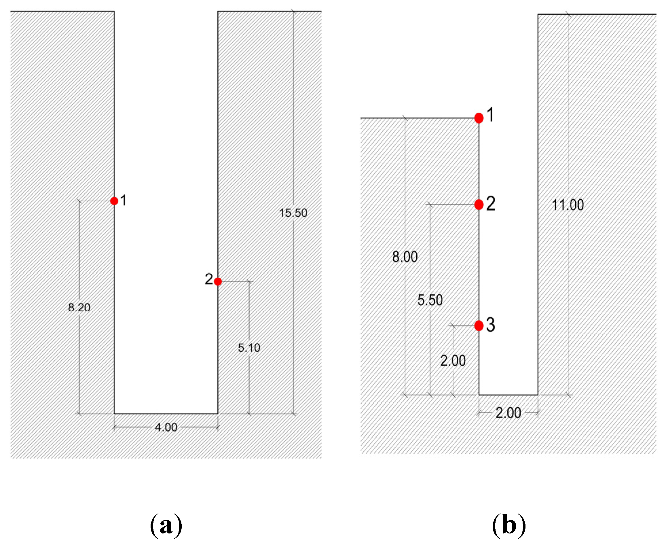
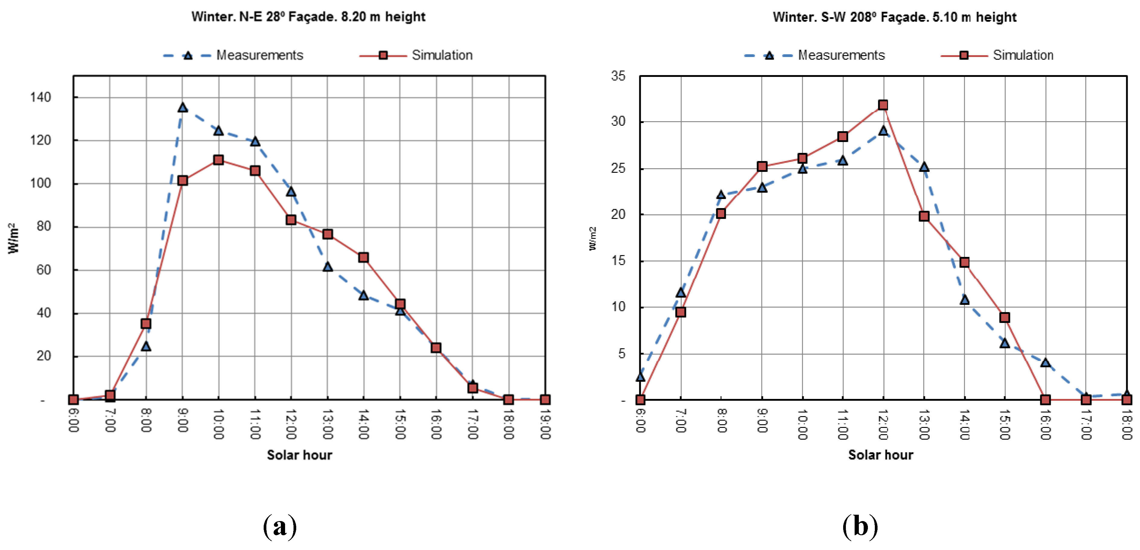
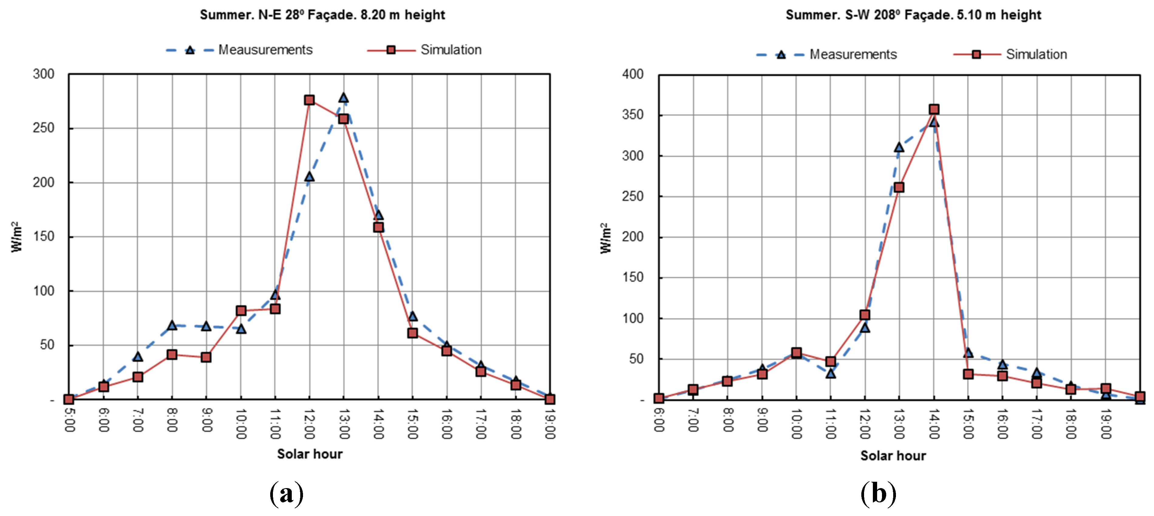
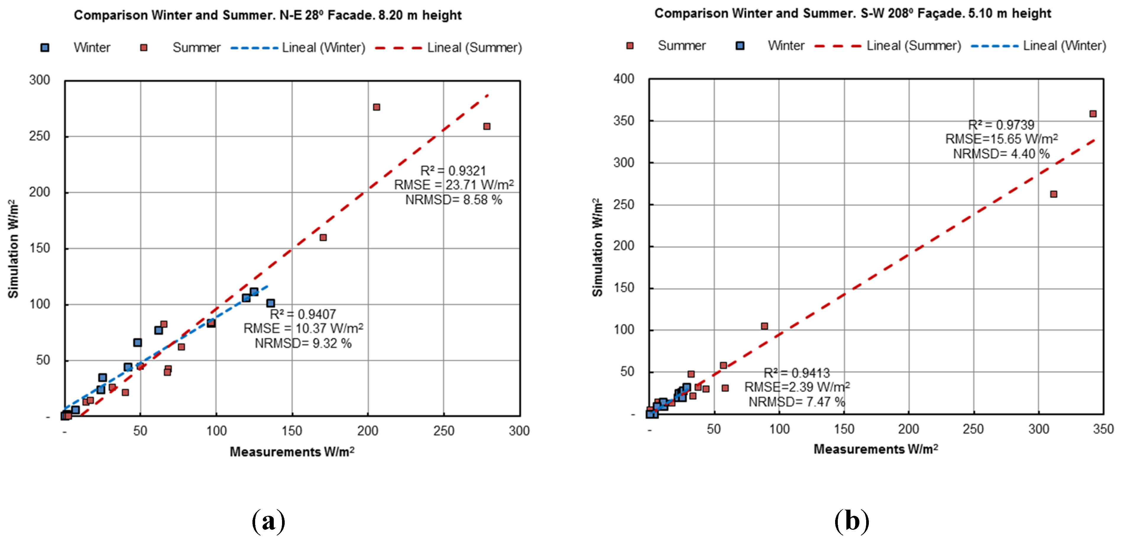
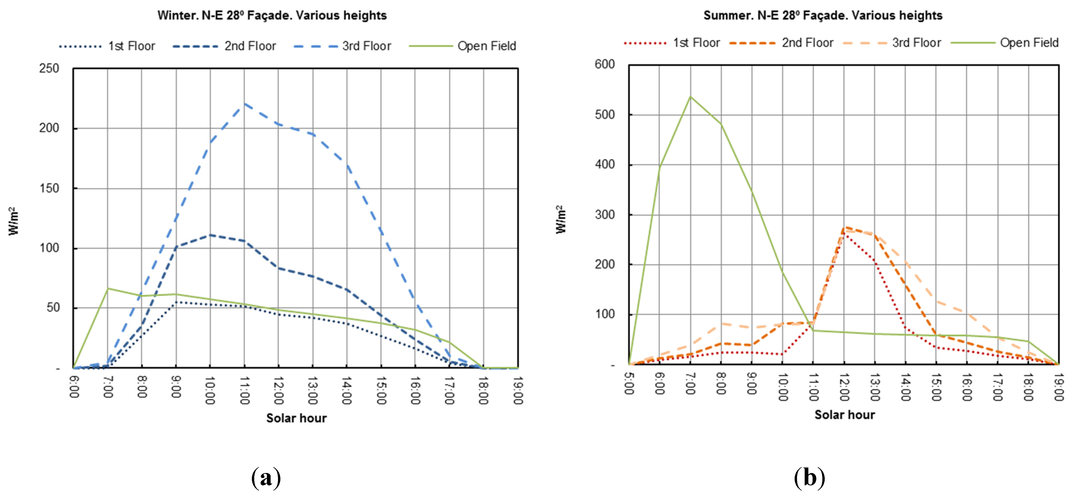
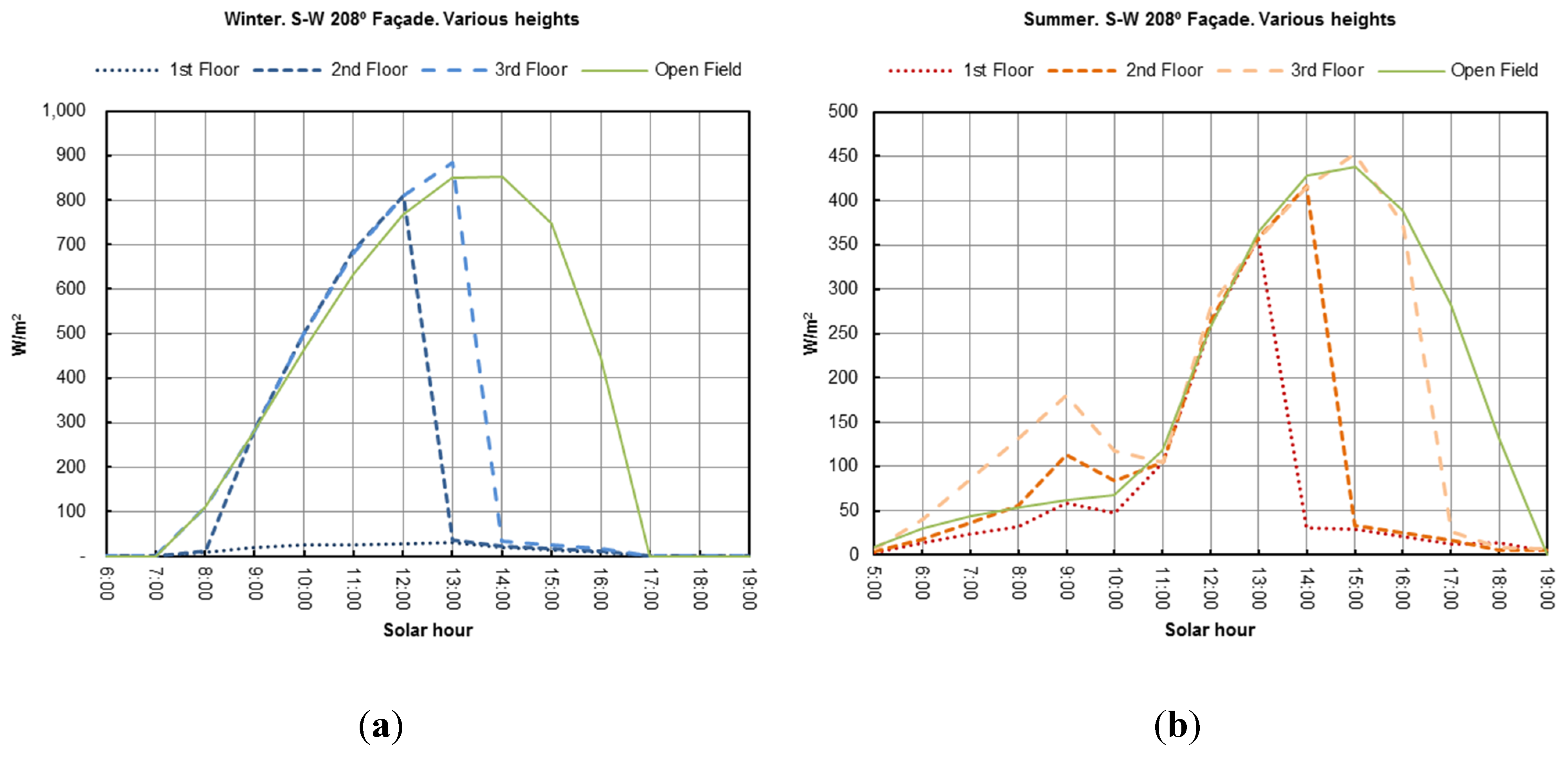
The DLSC of Cadiz is composed of 28º North-East and 208º South-West façades; H = 15.50 m, W = 4.00 m (Figure 6a). On-site measurement data were compared in both winter (Figure 7a,b) and summer (Figure 8a,b) at different heights. Cells were placed in the 28º North-East façade, with an altitude over the street level of 8.20 m and in the 208º South-West façade at 5.10 m. Cell measurements and simulations are also compared by means of Correlation R², RMSE and NRMSD (Figure 9a,b).

-

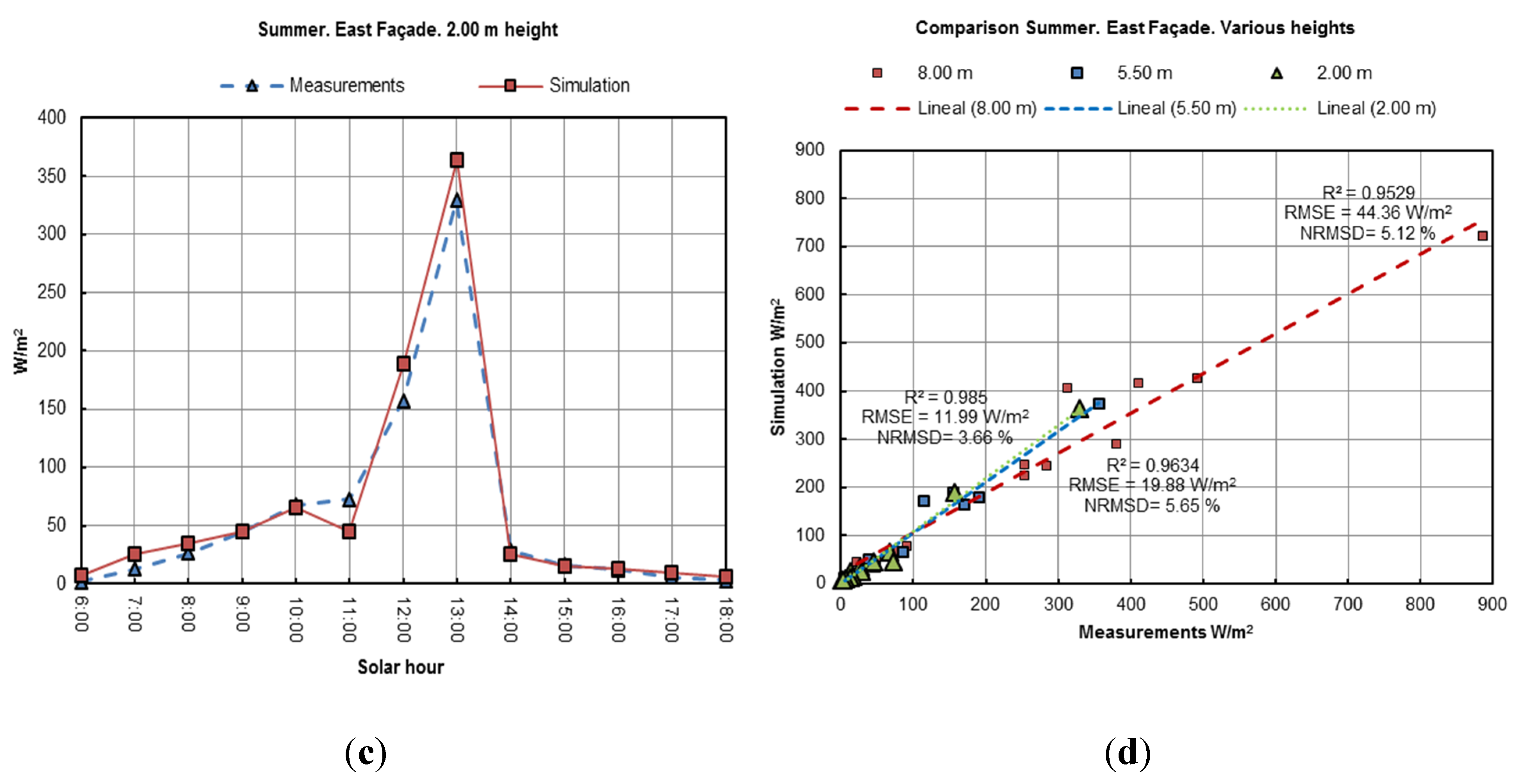
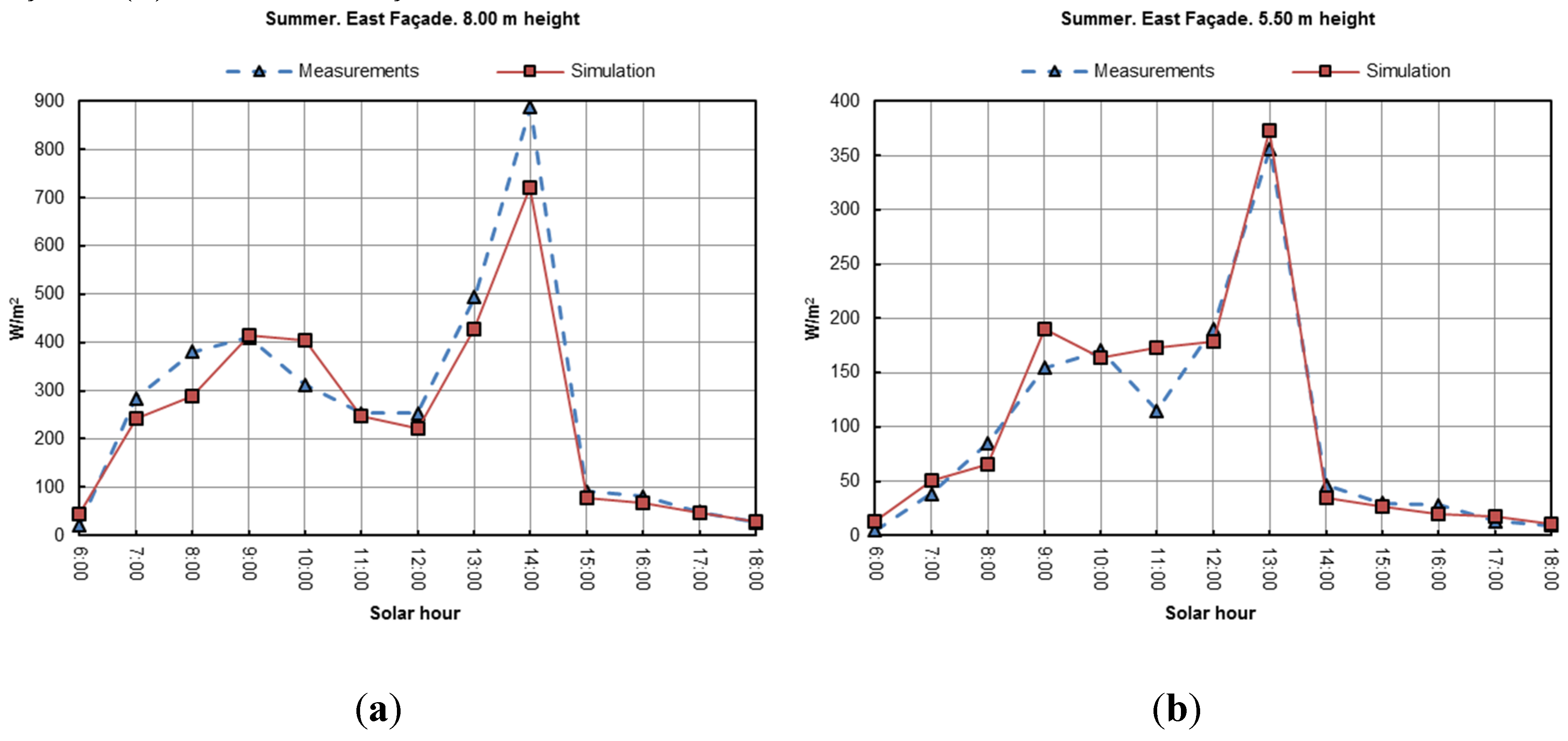
The DLSC of Seville is composed of East façade H = 8.00 m, (Figure 6b) were measurements cells were placed, West façade H = 11.00 m and W = 2.00 m. The second example for validation is an East façade during summer in an urban canyon of Seville. In this case, the comparison have done at different heights in the same façade; 8.00 m (Figure 10a); 5.50 m (Figure 10b), 2.00 m (Figure 10c) and by means of Correlation R², RMSE and NRMSD (Figure 10d).

Table 1. Data assumptions for validation

General Data		DLSC Geometry			Materials		Clear Sky Probability
DLSC	Orientation	H/W	L/H	Symmetry	Material	RC	Winter	Summer
Cádiz, Spain	N-E 28º Façade	3.875	9.67	Yes	Walls. Light paint, crème, grey	0.6	57%	80%
	S-W 208º Façade
Sevilla, Spain	East Façade	4.00	8.13	No	Street, asphalt, cobblestone	0.3	41%	86%

Table 1. Data assumptions for validation

General Data		DLSC Geometry			Materials		Clear Sky Probability
DLSC	Orientation	H/W	L/H	Symmetry	Material	RC	Winter	Summer
Cádiz, Spain	N-E 28º Façade	3.875	9.67	Yes	Walls. Light paint, crème, grey	0.6	57%	80%
	S-W 208º Façade
Sevilla, Spain	East Façade	4.00	8.13	No	Street, asphalt, cobblestone	0.3	41%	86%

Figure 6. Cell measurements location in Deep Long Street Canyons (a) Cadiz. 28º North-East façade at 8.20 m (1). 208º South-West façade at 5.10 m (2); (b) Seville East façade at 8.00 m (1), 5.50 m (2) and 2.00 m (3).

Figure 6. Cell measurements location in Deep Long Street Canyons (a) Cadiz. 28º North-East façade at 8.20 m (1). 208º South-West façade at 5.10 m (2); (b) Seville East façade at 8.00 m (1), 5.50 m (2) and 2.00 m (3).

Figure 7. 24 h comparison between cell measurements and simulations, winter in Cadiz. (a) N-E 28º Façade; (b) S-W 208º Façade.

Figure 7. 24 h comparison between cell measurements and simulations, winter in Cadiz. (a) N-E 28º Façade; (b) S-W 208º Façade.

Figure 8. 24 h comparison between cell measurements and simulations, summer in Cadiz. (a) N-E 28º Façade; (b) S-W 208º Façade.

Figure 8. 24 h comparison between cell measurements and simulations, summer in Cadiz. (a) N-E 28º Façade; (b) S-W 208º Façade.

Figure 9. R², RMSE and NRMSD between cell measurements and simulations in Cadiz. (a) N-E 28º Façade; (b) S-W 208º Façade.

Figure 9. R², RMSE and NRMSD between cell measurements and simulations in Cadiz. (a) N-E 28º Façade; (b) S-W 208º Façade.

Figure 10. 24 h comparison between cell measurements and simulations, summer. East façade. Seville. (a) 8.00 m height; (b) 5.50 m height; (c) 2.00 m height; (d) Correlation R², RMSE and NRMSD between cell measurements and simulations.

Figure 10. 24 h comparison between cell measurements and simulations, summer. East façade. Seville. (a) 8.00 m height; (b) 5.50 m height; (c) 2.00 m height; (d) Correlation R², RMSE and NRMSD between cell measurements and simulations.

Regarding the shape of the curve, simulated data reproduces the shape of the measurement curve in all graphics, with the following exceptions. In Figure 7a, between 9:00 and 10:00, simulated curve has an ascending pattern and simulated data shows a descending pattern. In Figure 8a, between 9:00 and 11:00, patterns for simulated and measured data do not match. Regarding the maximum and minimum values, they match in all comparisons, except for Figure 8a, where simulated data gives its maximum at 12:00 and real measurement at 13:00.

In the numerical values, the biggest errors that can be found in each cross-check are as follows. For Figure 7a, simulation gives 101.4 W/m² at 9:00 against a measured value of 135.7 W/m², which is a relative error of 25%; for Figure 7b, simulation gives an output of 31.9 W/m² at 12:00 against 29.1 W/m² for measured values, which means an error of 9%. For Figure 8a, simulation gives a simulated value of 276.3 W/m² against 206 W/m² at 12:00, which means an error of 25%; for Figure 8b, simulation gives an output of 311.62 W/m² at 12:00 against a measured value of 261.9 W/m², which is a relative error of 16%. For Figure 10a, simulation gives at 10:00 a value of 380.3 W/m² against a value of 290.0 W/m², which means an error of 24%; for Figure 10b, at 11:00 simulation gives an output of 172.6 W/m² against a value of 115.0 W/ m² for measured data, which means an error of 33%; for Figure 10c, simulated data at 11:00 is 44.5 W/m² against 72.3 W/m², which means an error of 39%.

High correlation R² values have been found between simulations and cell measurements; 0.9407, 0.9321 in 28º N-E façade (Figure 9a); 0.9413, 0.9739 in 208º S-W façade (Figure 9b) and 0.9529, 0.9850, 0.9634 in East façade (Figure 10d). Which foretells that numerical values from the simulation protocol are quite accurate.

Regarding Root Mean Square Error (RMSE) for each set of data, their values are depicted in Figure 9a, Figure 9b and Figure 10d. Their values are 23.71 W/m² in Summer and 10.37 W/m² in Winter (Figure 9a); 15.65 W/m² in Summer and 2.39 W/m² in Winter (Figure 9b); 44.36 W/m² in Summer and 19.88 W/m² in Winter (Figure 10d). Weighting these values using the Normalized Root Mean Square Deviation (NRMSD) the previous values are as follow: 8.58% in Summer and 9.32% in Winter (Figure 9a); 4.40% for summer and 7.47% for Winter (Figure 9b); 5.12% for 8.00 m height, 5.65% for 4.00 m height and 3.66% for 2.00 m height (Figure 10d).

Given these facts, the following remarks can be made regarding the accuracy of the calculation model. First, with respect to the pattern and shape of the curve, except for the mentioned exceptions, ascending and descending intervals match between both models, as well as the prediction for peak values. Secondly, regarding maximum relative error for each set of data, big deviations are found isolated at some point of the graphs, but they are not reproduce for the entire curve. The biggest mismatches are to be found when measuring small values, as in Figure 10c in the early morning, when the biggest relative error is to be found (39%). However, looking at the absolute values of RMSE and relative values of NRMSD, it can be seen that the simplified simulation model has, in general terms, an acceptable accuracies, with weighted errors that do not surpass 10%, with a maximum of 9.32% and a mean values of 6.31% for all sets of data combined together.

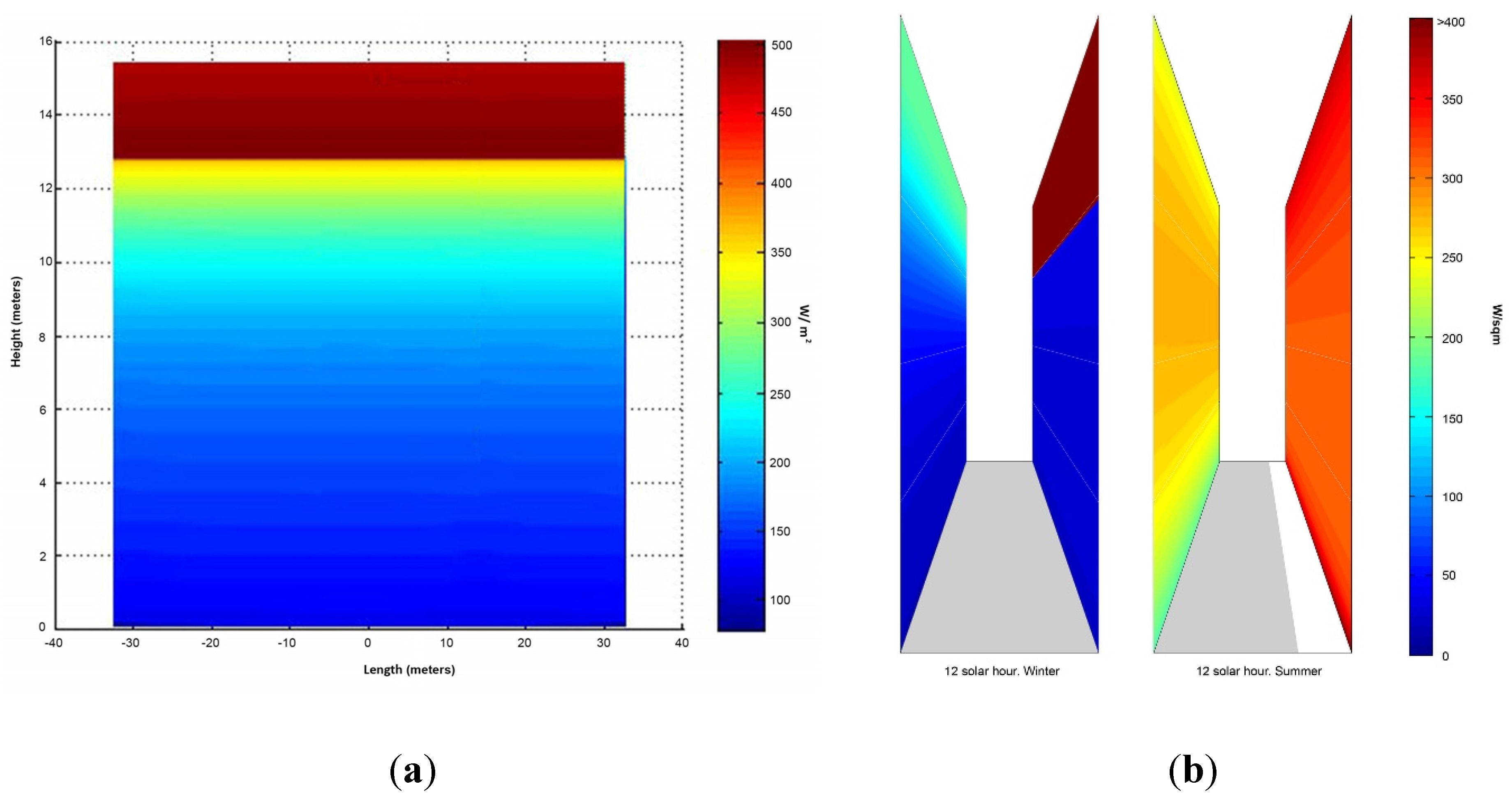
5.2. Model Applications. Simulations at Various Heights

This simulation model gives output values for every point of the façades surface. However, once the calculation model have been tested, the authors have considered useful, for the sake of clarity in the discourse, to generate data for various heights within a DLSC, both for winter and summer, and to compare them with the expected values for open field, in order to clarify the effect that DLSC have on the solar availability of these buildings. The results of these simulations are depicted in Figure 11 and Figure 12 for the location of Cadiz.

Figure 11. Simulations at various heights. Cadiz. (a) Simulation N-E 28º Façade, Winter; (b) Simulation N-E 28º Façade, Summer.

Figure 11. Simulations at various heights. Cadiz. (a) Simulation N-E 28º Façade, Winter; (b) Simulation N-E 28º Façade, Summer.

The aforementioned N-E façade features low radiation levels year-round, except for isolated peaks, when direct beams impinge on it. In winter (Figure 11a), openings in this façade should expect poor radiation levels, which is true, but only under two scenarios, open field or DLSC conditions in its lower rooms (1st floor), where radiation levels never rise beyond 62 W/m². The effect of the opposite façade, which greatly reflects radiation, can be clearly noticed in the second floor, where levels build up to 100 W/m² at midday, and in the 3rd floor, where figures above 200 W/m² can be found. In summer (Figure 11b), the effect of urban geometry in the first hours of morning was already remarked. Moreover, the lower the location of the simulated point is, the smaller radiation levels are found; in the first floor, values do not rise over 30 W/m² until noon, which means that urban geometry is used as a sort of solar protection and this comprises a reduction in the solar heat gains during the morning. After midday we find the opposite effect, that is, levels in the canyon exceed those in open field; the pattern of decay is similar at all levels, but with a more abrupt gradient depending on the position of the simulated point; that is, the lower the point, the more abrupt the pattern of decay.

Figure 12. Simulations at various heights. Cadiz. (a) Simulation S-W 208º Façade, Winter; (b) Simulation S-W 208º Façade, Summer.

Figure 12. Simulations at various heights. Cadiz. (a) Simulation S-W 208º Façade, Winter; (b) Simulation S-W 208º Façade, Summer.

208º S-W facing façade shows a typical behavior for this orientation, which is beneficial in terms of environmental performance; winter (Figure 12a) provides higher values for solar radiation (900 W/ m²), whereas in summer these values decrease to around 450 W/m². In this case, urban geometry loses solar gains for both seasons. Graphs are shaped basically by the fact that the simulated point receives direct beams of sun. In winter, values for open field respond to a sinusoidal distribution. In 2nd and 3rd floor, it is truncated from the time when the opposite façade blocks direct sun, whilst 1st floor never receives direct solar radiation. In this situation, available energy comes only from diffuse and reflected components, causing these points to achieve scarce light; this fact reveals crucial, particularly on the ground floor, where the maximum value for winter is only 32 W/m². In summer (Figure 12b), distribution for the open field follows a pattern that shows a steady increase during the morning hours, and peak values in the afternoon, when direct radiation impinges on this façade. Urban geometry has a double effect on these figures. In the morning hours the reflected component from the opposite façade, the one that receives direct solar radiation, cause levels to increase from around 62.50 W/m² (open field) to 112.70 W/ m² (2nd floor) and 179.70 W/m² (3rd floor). In the afternoon, peak values are found around 15:00 for open field, while levels on the rest of the floors fall abruptly, depending at the time when directs beams are obstructed by the opposite façade.

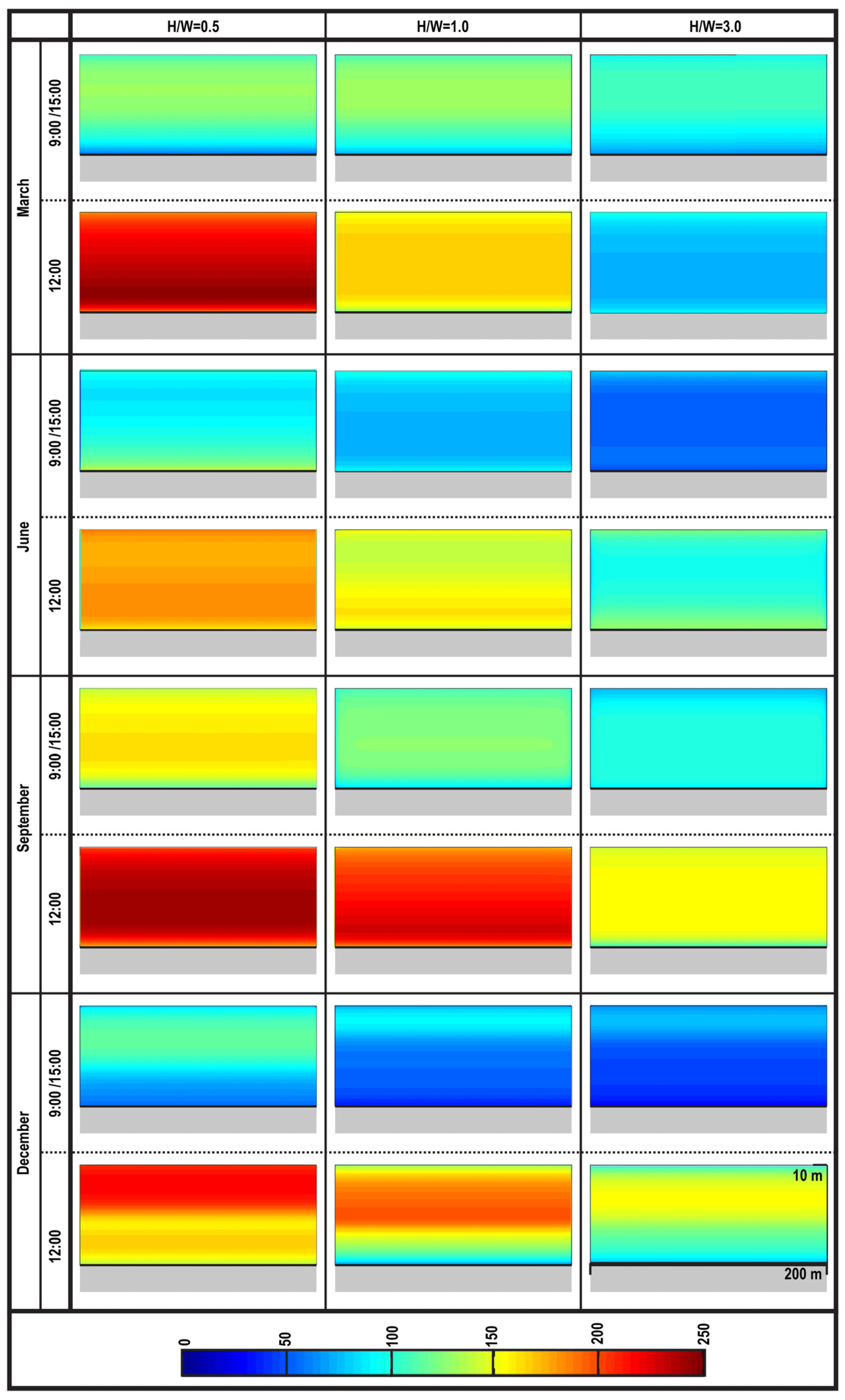
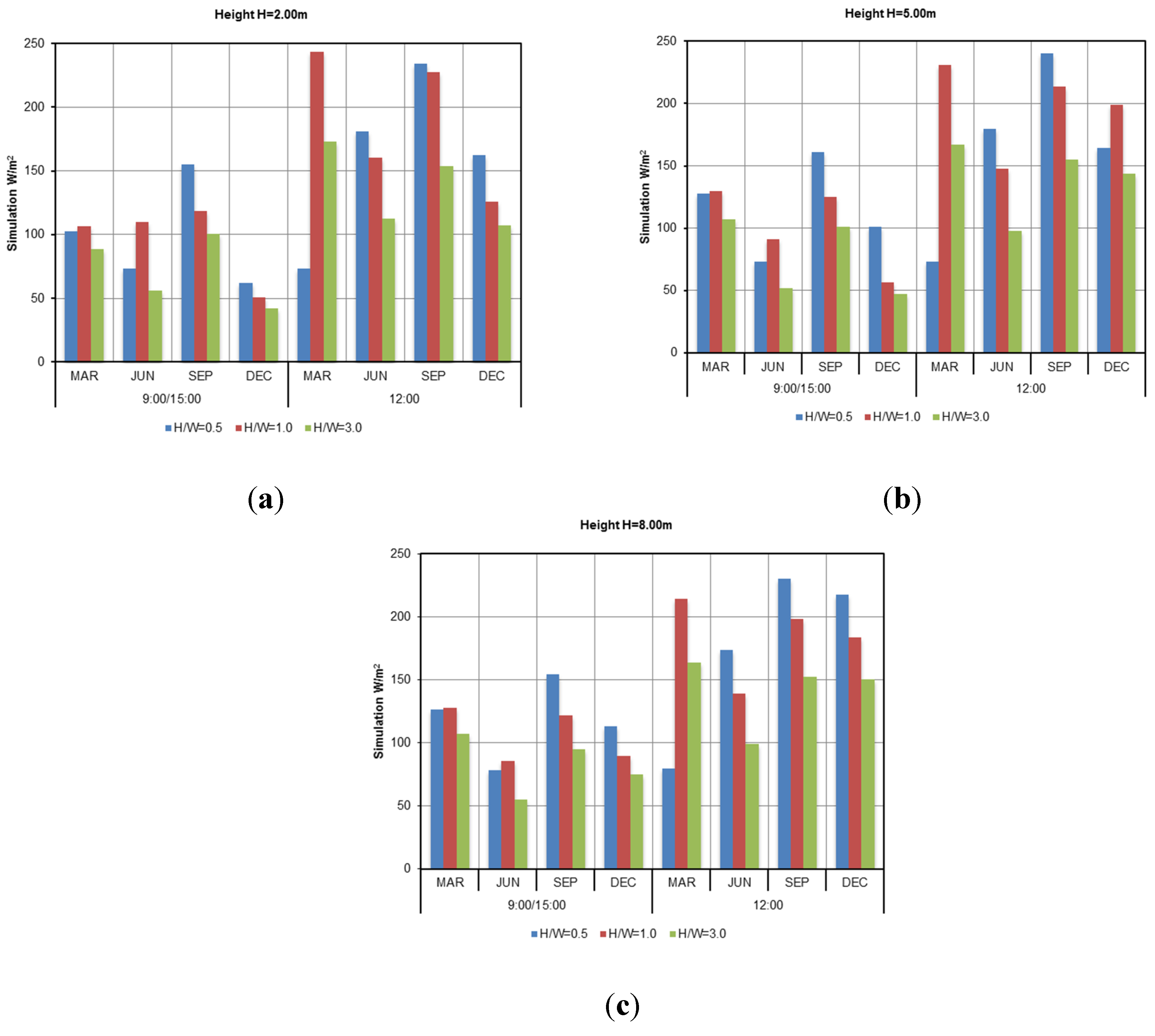
5.3. Simulations Results. Parametric Analysis

In order to further present the functionality and capabilities of the model, a parametric analysis has been conducted for a theoretical street canyon, located in the city of Seville oriented though a E-W axis, with a length of 200 m and two parallel façades with a height of 10 m. The variable parameter in this case is the width of the canyon, which varies from 20 m, 10 m and 3.30 m; hence, three types of street canyons are analyzed, H/W = 0.5, H/W = 1.0 and H/W = 3.0, respectively. Data has been simulated for four months in a period of one year (March, June, September and December) in order to have a representative month for each season of the year; for each one of these months, three hours of the day have been simulated (9:00, 12:00 and 15:00 for solar time). For the sake of simplicity and due to solar geometry, data regarding 9:00 and 15:00 are the same, and they are presented together. Figure 13 represents data for radiation in the façade of the street canyon that faces south. Simulations have been performed for the most probable sky scenario for each considered month, according to the data provided by EPW files for the location of Seville. Results are presented graphically in Figure 13 and Figure 14.

Figure 13. Parametric analysis for different widths of street canyons. South façade, Seville. (W/m²)

Figure 13. Parametric analysis for different widths of street canyons. South façade, Seville. (W/m²)

From each of these simulations, data has been extracted for point situated in a height of H = 2.00 m, H = 5.00 m and H = 8.00 m, which would correspond to the ground, first and second floor of a building located within the simulated street canyon.

Figure 14. Results from the parametric analysis. South façade, Seville. (a) Point at height H = 2.00 m; (b) Point at height H = 5.00 m; (c) Point at height H = 8.00 m.

Figure 14. Results from the parametric analysis. South façade, Seville. (a) Point at height H = 2.00 m; (b) Point at height H = 5.00 m; (c) Point at height H = 8.00 m.

6. Discussion and Conclusion

6.1. Validity of the Method

According to the results, it can be stated that, in general terms, the proposed method has been validated for the given boundary conditions. This validity relies on some key points that the authors consider worth explaining.

• First, users only need to input some data, regarding solar radiation, geometrical characteristics of the street canyon and RC of the materials, in order to make use of the calculation routine; this makes a difference, as it is not necessary to model 3D geometry, a task that usually requires a considerable amount of time.
• Secondly, this model does not make use of any theoretical abstractions (such as pepper point diagrams, radiosity, etc.), which is easier to understand, and also allows for direct check against measured data.

6.2. Accuracy of the Method

The proposed simplified calculation method has proven to be accurate in terms of adjustment to the pattern of the data curve and the expected numerical values, except minor deviations.

Comparison between the set of data reveal that the calculation routine reproduces with acceptable accuracy the behavior of solar radiation within the façades of the buildings inside street canyons.

• Balance between simplification of the geometry and accuracy of the model. When trying to simulate some phenomenon of the real world, some simplification has to be made in order to attain a simulation model that is acceptable in terms of computing cost. In this model, despite having certain degree of simplification, such as taking weighted average values of reflections coefficients or merging irregularities of the real façade with their main plane, the analysis of the results of the model has proven that it has an acceptable accuracy, and also that outputs are consistent and coherent, according to parametric analysis.
• Acceptable accuracy of the model after comparing with real measurements. Other point that has proven to be a cornerstone in this research is the comparison of results with on-site real measurements. Even when a simulation model gives physically reasonable results, it is always advisable to compare with real conditions. In this case, cross-checking against two real case-studies, two street canyons located in two Southern European cities, have proven that the model reproduces the behavior of radiation interchanges with acceptable accuracy, even when for some specific times and situations results may differ. These errors can be explained and their degree of uncertainty, in the whole, is acceptable, with average values about 6% of the total.
• Possibility of simulating several types of street canyons without having to prepare several 3D models. Useful for parametric analysis and research purposes. Other main outcome that can be considered useful in terms of computing and time cost is the possibility of calculating radiant distribution in a façade without the necessity of making a 3D model in a computer CAD program, and therefore importing into the model. In this case, the model constructs the scenario only with numerical data, which is faster to input. In addition, input data can be stored in matrixes and then one or more variables can be set free to perform a bench test or a parametric analysis, such in this case in point 5.3. This can be useful to research purposes which usually requires handling bigger amounts of data.

6.3. Future Improvements

The proposed method has some inaccuracies that should be taken into consideration, although they do not compromise the accuracy of the model. Simulated data does not exactly fit the measured ones, but error margin can be considered as acceptable; this can be can be attributed to various facts. First, singularities in the real model, as real building façades are not perfect planes, and have many irregularities, changes of materials and protruding elements Secondly, theoretical values of radiant properties of the materials may not be an exact figure, as those one considered in the simulation. Thirdly, and the spectral response of the measurement cells can lead to minor bias, particularly in presence of high temperatures. In every simulation process, a balance between accuracy and calculation speed is one of the key factors, and in this case this point has proven to be crucial. Under a critical eye, the authors consider that this method has been validated to calculate solar radiation availability in façades located within street canyons with simple geometries, but further research is needed to consider other sky conditions and specific cases in an urban grid. i.e., cross-streets or short urban canyons, which are not considered in our simulation software, constitute future developments.

In turn, the proposed simulation methodology has proven to be valid under high solar radiation conditions. Conditions for the open field are not applicable in this case, as the pattern for solar radiation in the façades of these buildings differs greatly from those. Despite this dwellings are located in an urban grid, it does not represent a burden on solar access; considerable amounts of solar radiation impinges on the façades at different heights, which has a decisive importance on passive design strategies, such as solar gains and thermal lag.

In this study, the authors developed a predictive simulation tool that allows achieving the radiant values of a façade located within any street canyon under high solar radiation conditions. This software is deemed important to understand the environmental performance of architectural envelope of buildings. As can be seen in the proposed example, a deep urban canyon located in a sunny climate, the correlation between simulated and measured values are creatively close, considering the singularities in the real model, theoretical values of radiant properties and/or the spectral response of the measurement cells.

References

1. Littlefair, P. Daylight, sunlight and solar gain in the urban environment. Sol. Energy 2001, 70, 177–185. [Google Scholar] [CrossRef]
2. Strømann-Andersen, J.; Sattrupb, P.A. The urban canyon and building energy use: Urban density versus daylight and passive solar gains. Energy Build. 2011, 43, 2011–2020. [Google Scholar] [CrossRef]
3. Hviid, C.A.; Nielsen, T.R.; Svendsen, S. Simple tool to evaluate the impact of daylight on building energy consumption. Sol. Energy 2008, 82, 787–798. [Google Scholar] [CrossRef]
4. Attia, S.; Hensen, J.L.M.; Beltrán, L.; De Herde, A. Selection criteria for building performance simulation tools: Contrasting architects' and engineers' needs. J. Build. Perform. Simul. 2012, 5, 155–169. [Google Scholar] [CrossRef] [Green Version]
5. Ochoa, C.E.; Aries, M.B.C.; Hensen, J.L.M. State of the art in lighting simulation for building science: A literature review. J. Build. Perform. Simul. 2012, 5, 209–233. [Google Scholar] [CrossRef]
6. Nicholson, S.E. A pollution model for street-level air. Atmos. Environ. 1975, 9, 19–31. [Google Scholar] [CrossRef]
7. Li, D.H.W.; Cheung, G.H.W.; Lam, J.C. Simple method for determining daylight illuminance in a heavily obstructed environment. Build. Environ. 2009, 44, 1074–1080. [Google Scholar] [CrossRef]
8. Bozonnet, E.; Belarbi, R.; Allard, F. Modelling solar effects on the heat and mass transfer in a street canyon, a simplified approach. Sol. Energy 2005, 79, 10–24. [Google Scholar] [CrossRef]
9. Petersen, S.; Mommea, A.J.; Hviid, C.A. A simple tool to evaluate the effect of the urban canyon on daylight level and energy demand in the early stages of building design. Sol. Energy 2014, 108, 61–68. [Google Scholar] [CrossRef]
10. Herrmann, J.; Matzarakis, A. Mean radiant temperature in idealised urban canyons—Examples from Freiburg, Germany. Int. J. Biometeorol. 2012, 56, 199–203. [Google Scholar] [CrossRef] [PubMed]
11. Vardoulakis, S.; Fisherb, B.E.A.; Pericleousa, K.; Gonzalez-Flescac, N. Modelling air quality in street canyons: A review. Atmos. Environ. 2003, 37, 155–182. [Google Scholar] [CrossRef]
12. Stasiek, J.A. Application of the transfer configuration factors in radiation heat transfer. Int. J. Heat Mass Transf. 1998, 41, 2893–2907. [Google Scholar] [CrossRef]
13. Miguet, F.; Groleau, D. A daylight simulation tool for urban and architectural spaces—application to transmitted direct and diffuse light through glazing. Build. Environ. 2002, 37, 833–843. [Google Scholar] [CrossRef]
14. Cabeza-Lainez, J.M.; Pulido-Arcas, J.A.; Rubio-Bellido, C.; Castilla, M.V.; Gonzalez-Boado, L.; Sanchez-Montañes, B. New Computational Techniques for Solar Radiation in Architecture. Sol. Radiat. Appl. 2015. [Google Scholar] [CrossRef]
15. Bradley, A.V.; Thornes, J.E.; Chapman, L. A method to assess the variation of urban canyon geometry from sky view factor transects. Atmos. Sci. Lett. 2001, 2, 155–165. [Google Scholar] [CrossRef]
16. Cabeza-Lainez, J.M. Fundamentos de Transferencia Radiante Luminosa (Including Software for Simulation); Netbiblo: La Coruña, Spain, 2010. [Google Scholar]
17. Perez, R.; Ineichen, P.; Seals, R.; Michalsky, J.; Stewart, R. Modeling daylight availability and irradiance components from direct and global irradiance. Sol. Energy 1990, 44, 271–289. [Google Scholar] [CrossRef]
18. Cabeza-Lainez, J.M.; Pulido-Arcas, J.A.; Sanchez-Montañes, B.; Rubio-Bellido, C. New configuration factor between a circle and a point-plane at random positions. Int. J. Heat Mass Transf. 2014, 69, 147–150. [Google Scholar] [CrossRef]
19. Cabeza-Lainez, J.M.; Pulido-Arcas, J.A.; Castilla, M.V. New configuration factor between a circle, a sphere and a differential area at random positions. J. Quant. Spectrosc. Radiat. 2013, 129, 272–276. [Google Scholar] [CrossRef]
20. Cabeza-Lainez, J.M.; Pulido-Arcas, J.A. New configuration factors for curved surfaces. J. Quant. Spectrosc. Radiat. 2013, 117, 71–80. [Google Scholar] [CrossRef]
21. Howell, J.R.; Siegel, R.; Menguc. Thermal Radiation Heat Transfer. Available online: www.thermalradiation.net (accessed on 5 September 2015).
22. Chekhovskii, I.R.; Sirotkin, V.V.; Chu-Dun-Chu, Iu.V.; Chebanov, V.A. Determination of radiative view factors for rectangles of different sizes. High Temp. Sci. 1979, 17, 97–100. [Google Scholar]
23. Chung, B.T.F.; Kermani, M.M. Radiation view factors from a finite rectangular plate. J. Heat Transf. 1989, 111, 1115–1117. [Google Scholar] [CrossRef]
24. Ehlert, J.R.; Smith, T.F. View Factors for Perpendicular and Parallel, Rectangular Plates. J. Thermophys. Heat Transf. 1993, 7, 173–174. [Google Scholar] [CrossRef]
25. Gross, U.; Spindler, K.; Hahne, E. Shapefactor-equations for radiation heat transfer between plane rectangular surfaces of arbitrary position and size with parallel boundaries. Lett. Heat Mass Transf. 1981, 8, 219–227. [Google Scholar] [CrossRef]
26. Hsu, C.-J. Shapefactor-equations for radiant heat transfer between two arbitrary sizes of rectangular planes. Can. J. Chem. Eng. 1967, 45, 58–60. [Google Scholar] [CrossRef]
27. Yáñez Paradeda, G. Arquitectura Solar e Iluminación Natural: Conceptos, Métodos y Ejemplos; Munillaleria: Madrid, Spain, 2008. [Google Scholar]
28. Rubio-Bellido, C.; Pulido-Arcas, J.A.; Cabeza-Lainez, J.M. Adaptation Strategies and Resilience to Climate Change of Historic Dwellings. Sustainability 2015, 7, 3695–3713. [Google Scholar] [CrossRef]
29. Lambert, J.H. 1760 Photometria; Di Laura, D., Ed.; Illuminating Engineering Society of North America: New York, NY, USA, 2001. (In Latin) [Google Scholar]
30. Walton, G.N. A new algorithm for radiant interchange in rooms loads calculations. ASHRAE Trans. 1980, 86, 190–208. [Google Scholar]