On the Implementation of Variable Speed in Pump-Turbine Units Providing Primary and Secondary Load-Frequency Control in Generating Mode

Abstract

This paper analyses different control strategies for the speed control loop of a variable-speed pump-turbine unit equipped with a doubly fed induction generator, operating in generating mode in an isolated power system with high penetration of intermittent renewable energy. The control strategies are evaluated and compared to each other in terms of the amount of water discharged through the pump-turbine and of the wicket gates fatigue while providing primary and secondary load-frequency control. The influence of the penstock length and the initial operating point on the performance of each control strategy is studied in detail. For these purposes, several simulations have been performed with a suitable dynamic model of the pumped-storage hydropower plant and the power system. The results of the paper indicate that a proper control strategy would consist in updating the reference speed according to the power generation schedule and keeping it constant within each scheduling period (typically 1 h).

1. Introduction

The integration of intermittent energy sources in the grid is one of the most important challenges for hydropower plants nowadays [1]. Excess wind and solar energy is a real fact, especially in isolated systems, such as small or medium size island electric power systems [2]. The penetration of these intermittent sources is very high in order to avoid environmental and social costs of fossil fuel-based electricity generation [3,4]. Pumped storage hydropower plants (PSHPs) are useful to hedge against the uncertainty in intermittent renewable energy (wind and solar) [5]. PSHPs can contribute significantly to the load-frequency control in generating mode. In pumping mode, variable-speed or hydraulic short-circuit operation is required to provide load-frequency control [6,7].

Doubly fed induction generators (DFIG) are widely used for variable speed pumped-storage units [8,9]. In [10] two control schemes are proposed for variable speed pumped-storage units operating in generating mode. In the load control scheme, the power injected into the grid is regulated by the rotor-side converter and the turbine governor is in charge of restoring the unit running speed to the reference value. In this way, the electric power delivered by the unit is free from water hammer effects since the variations in the turbine mechanical power are absorbed by the inertia of the rotational masses. In addition, the reference speed can be modified in a speed control loop in order to increase the hydraulic efficiency [11].

The dynamic response of a PSHP equipped with a DFIG and load control scheme has been analyzed in detail in [12,13,14]. In [12,13] the speed reference is kept constant during the simulations, whereas in [14] only a sudden decrease of the active power set point is simulated. There are therefore several questions regarding the speed control loop which have not been answered yet. Variable speed pumped-storage units are expected to provide primary and secondary load-frequency control both in generating and pumping mode. As it is well known, variable speed allows increasing the efficiency in turbine mode. However, to authors’ knowledge there is no previous work on how to update the reference speed of a hydropower unit when it provides load-frequency control, as most hydropower units do. How often the optimal speed (as referred to in [14]) should be updated in order to provide primary and secondary load-frequency control in an optimum way is the main question addressed in this paper. In order to ask this question, it is necessary to define a criterion to evaluate the performance of the pump-turbine unit. The criterion used in this paper for this purpose is based on the amount of water discharged through the pump-turbine, and on the fatigue of the wicket gates servo mechanism, while providing load-frequency control: the lower the water usage (and therefore the necessary energy consumption for pumping) and the wicket gates fatigue, the better the pump-turbine performance, provided that the response meets certain quality standards.

This paper studies and compares to each other different control strategies for the speed control loop of a PSHP equipped with a pump-turbine and a DFIG when it operates in generating mode. The PSHP is connected to a small isolated power system with thermal, wind and solar generation, and which provides secondary load-frequency control under the orders of an automatic generation control (AGC) system.

A dynamic model of the PSHP and the power system has been developed and several simulations have been carried out in order to evaluate and compare to each other the proposed control strategies. Moreover, the influence of the initial operating point (initial power and gross head) and the penstock length on the performance of each control strategy has been analyzed in detail.

The remainder of the paper is organized as follows: in Section 2, the main characteristics of the PSHP and the power system where the study is carried out are presented; in Section 3 the non-linear dynamic model of the considered power system is described; the control strategies formulated for the speed control loop are described in Section 4; the simulations carried out in this study are described in Section 5; the results of the simulations are presented in Section 6; finally, the main conclusions of the paper are summarized in Section 7.

2. Description of the Pumped Storage Hydropower Plant and the Power System

The PSHP modelled in this paper is equipped with a pump-turbine unit coupled to a DFIG and the rated power of the unit is 14.97 MW. Two solutions with different penstock length (1350-m and 300-m) have been studied in order to gain insight on the influence of the conduit water inertia on the dynamic response of the PSHP. There is no surge tank in the scheme and the tail race tunnel is not considered due to its short length. The power system to which the PSHP is connected comprises six fuel-oil generating units, five diesel-oil generating units, seven gas-oil generating units and two combined cycle gas units. The total installed thermal generation power in July 2012 was 852 MW [7]; in addition, there were 35 MW and 24 MW of wind and photovoltaic generation at that time.

3. Dynamic Model

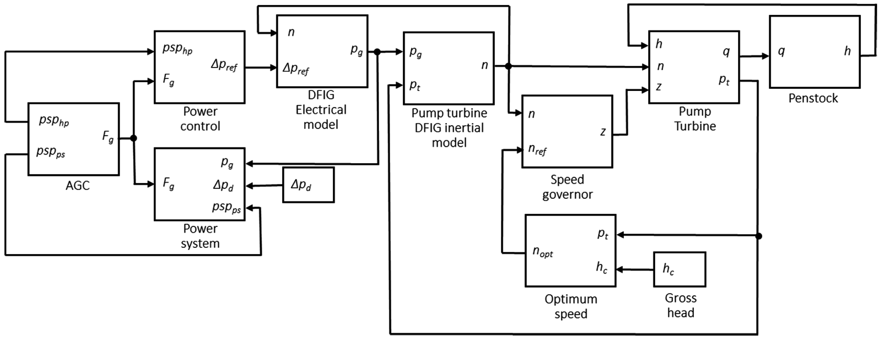
Figure 1 shows the block diagram of the simulation model developed in Matlab-Simulink. Each block of the diagram is briefly described below.

3.1. Penstock

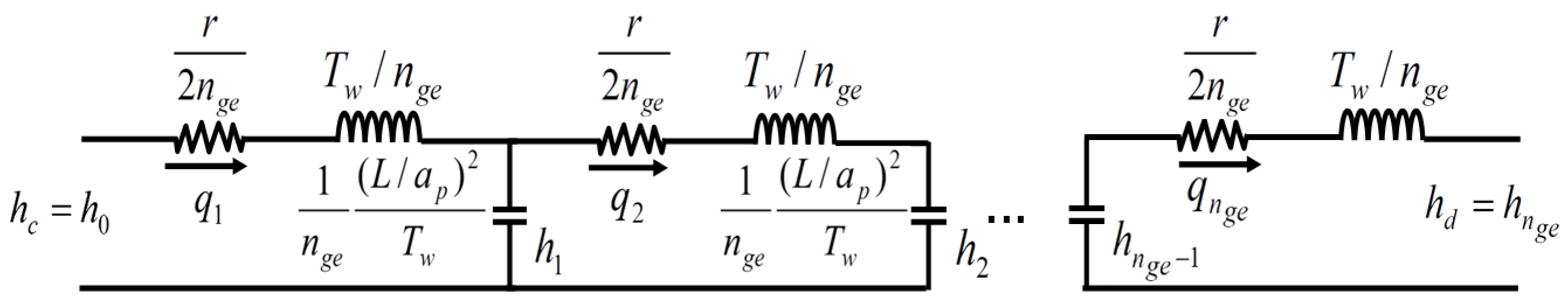
Hydraulic transients in close conduits are properly described by a couple of partial differential equations, usually referred to as mass and momentum conservation equations [15]. In this paper, a lumped parameters model has been used to transform the above-mentioned system of partial differential equations in a system of ordinary differential equations [13,16]. For the long penstock configuration, the penstock has been modelled through Equations (1) and (2), considering ten Г-shaped consecutive elements (n_ge = 10), Figure 2 [7,17].

Figure 1. Block diagram of the dynamic model. All variables are expressed in p.u. values with respect to the base values included in Table 1.

Figure 1. Block diagram of the dynamic model. All variables are expressed in p.u. values with respect to the base values included in Table 1.

Table 1. Model base values.

Parameter	Value	Parameter	Value
Qb	10 m3/s	Pb (base power)	14.93 MW
Hb	165.19 m	Fb (base frequency)	50 Hz
Nb (base running speed)	600 r.p.m	D (turbine diameter)	1.31 m

Table 1. Model base values.

Parameter	Value	Parameter	Value
Qb	10 m3/s	Pb (base power)	14.93 MW
Hb	165.19 m	Fb (base frequency)	50 Hz
Nb (base running speed)	600 r.p.m	D (turbine diameter)	1.31 m

Figure 2. Scheme of the long penstock model.

Figure 2. Scheme of the long penstock model.

$$\frac{\text{d}{q}_i}{\text{d}t}=\frac{n_{\text{ge}}}{T_{\text{w}}}\left(h_{i-1}-h_i-\frac{r}{2n_{\text{ge}}}{q_i}^2\right)\text{ and }{T}_{\text{w}}=\frac{L}{gF}\frac{Q_{\text{b}}}{H_{\text{b}}}$$

(1)

$$\frac{\text{d}{h}_i}{\text{d}t}=\frac{T_{\text{w}}{n}_{\text{ge}}}{{T_{\text{e}}}^2}\left(q_i-q_{i+1}\right)\text{ and }{T}_{\text{e}}=\frac{L}{a_{\text{p}}}$$

(2)

In Equations (1) and (2), n_ge is the number of elements, h_i (p.u.) is the head at the end of the i-th Γ element, q_i (p.u.) is the flow in the i-th Γ element, T_w (s) is the water starting time, L (m) is the penstock length, g (m/s²) is the gravity acceleration, F (m²) is the penstock cross section, Q_b (m³/s) is base flow, H_b (m) is the base head, T_e (s) is the water elastic time, a_p (m/s) is the penstock wave speed and r (p.u.) is twice the head loss in the penstock with rated flow.

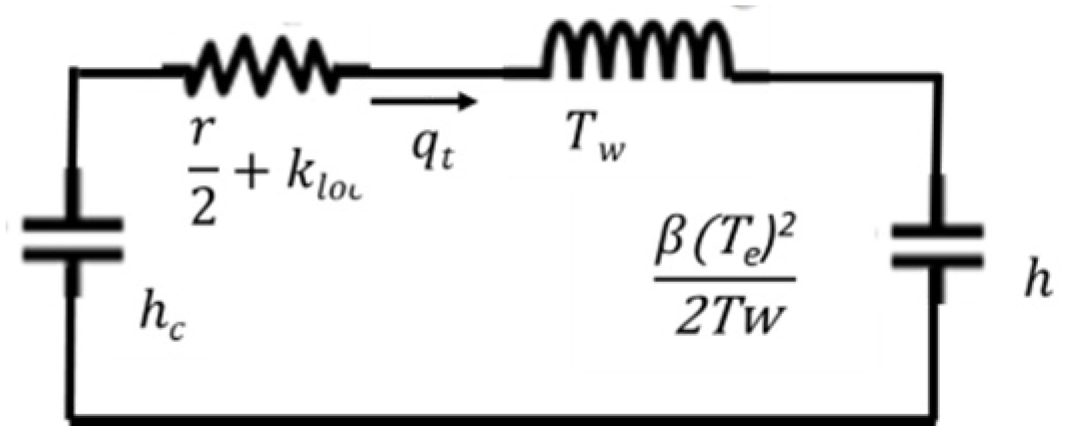
For the short penstock configuration, the penstock has been modelled through Equations (3) and (4), considering a single Π-shaped element, Figure 3. The element has one series branch and two shunt branches. The total head losses are included in the series branch of Equation (3), whereas the elasticity effects are included in the shunt branches of Equation (4). Expression in Equation (4) includes a correction coefficient β to match the first peak of the frequency response of the continuous model [18].

Figure 3. Scheme of the short penstock model.

Figure 3. Scheme of the short penstock model.

$$\frac{\text{d}{q}_t}{\text{d}t}=\frac{1}{T_{\text{w}}}\left(h_{\text{c}}-h-\frac{r}{2}{q}_{\text{t}}\left|q_{\text{t}}\right|\right)$$

(3)

$$\frac{\text{d}h}{\text{d}t}=\frac{2T_{\text{w}}}{\mathsf{\beta }{T_{\text{e}}}^2}\left(q_{\text{t}}-q\right)\text{ where }\mathsf{\beta }=\frac{8}{{\pi }^2}$$

(4)

In Equations (3) and (4), h_c is the gross head, h is the net head at the pump-turbine inlet, q_t is the flow in the penstock, and q is the flow through the pump-turbine.

3.2. Pump-Turbine

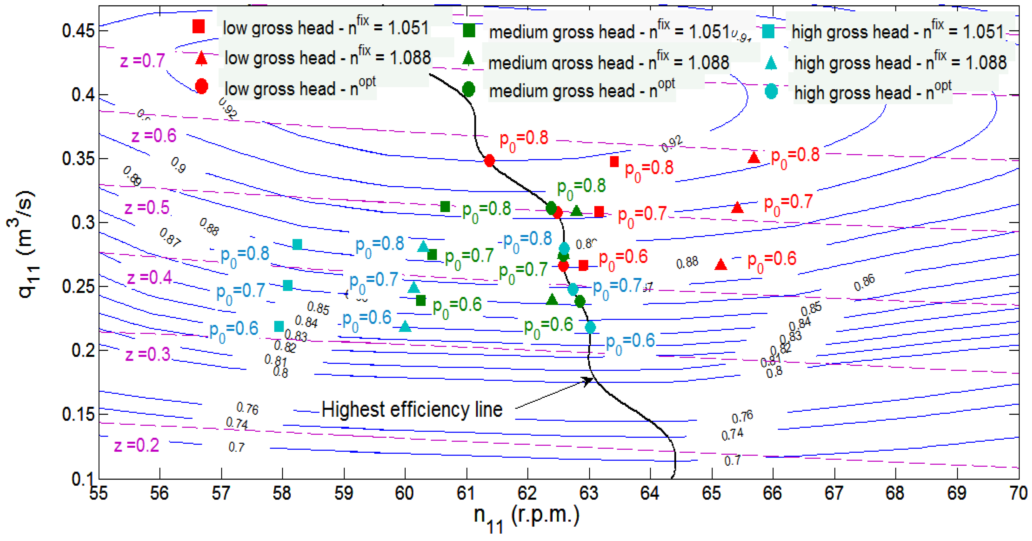
The performance curves of the pump-turbine unit in generating mode have been approximated by those used in [17] and are shown in Figure 4. In this case the hill chart, expressed as a function of the unit speed n₁₁ and flow q₁₁ in Equation (5), is experimental, where z is the wicket gates position. In the absence of experimental data, the selection of the pump-turbine model can be crucial to accurately predict its behavior with variable speed [19].

Figure 4. Pump-turbine performance curves in generating mode; considered initial operating points superimposed in the curves.

Figure 4. Pump-turbine performance curves in generating mode; considered initial operating points superimposed in the curves.

The “pump-turbine” block calculates the flow discharged through the pump-turbine runner q, as well as the shaft mechanical power p_t, by interpolating in the above-mentioned performance curves. Turbine dynamics has been neglected.

$$n_{11}=\frac{nD}{\sqrt{H}}{q}_{11}=\frac{q}{D^2\sqrt{H}}$$

(5)

3.3. Optimal Speed

The “optimal speed” block determines the optimal running speed of the unit for a given mechanical power p_t and gross head h_c, by interpolating iteratively in the pump-turbine performance curves. The optimal running speed is defined as the one which allows generating the given mechanical power with the highest efficiency, or rather, with the lowest water discharge. The block searches for the optimal speed within the pump-turbine hill chart, which have been previously parameterized.

3.4. Pump-Turbine-Doubly Fed Induction Generator Inertial Model

The “pump-turbine-DFIG inertial model” block calculates the unit running speed n from the unbalance between the electrical power delivered to the grid p_g and the shaft mechanical power p_t in Equation (6):

$$T_{\text{m}}\cdot \frac{\text{d}n}{\text{d}t}\cdot n=p_{\text{t}}-p_{\text{g}}$$

(6)

T_m (s) is the mechanical starting time of the unit.

3.5. Speed Governor

The control diagram proposed in [10] for the speed governor of a hydro unit with DFIG is used in the present work. The “optimal speed” block sends the reference speed n^ref to the “speed governor” block and a conventional PI controller in Equation (7) acts on the wicket gates opening z in order to follow the optimal speed signal:

$$\frac{\text{d}\Delta z}{\text{d}t}=\frac{\text{1}}{\mathsf{\delta }}\frac{\text{d(}{n}^{\text{ref}}-n)}{\text{d}t}+\frac{\text{(}{n}^{\text{ref}}-n)}{\mathsf{\delta }{T}_{\text{r}}}$$

(7)

The controller gains are expressed in terms of the parameters used to model the classical mechanical hydraulic governor, δ is transient speed drop, and T_r (s) is dashpot time constant. Two different pairs of controller gains have been used depending on the penstock length.

3.6. Power Control

The changes in the electrical power required to the DFIG Δp_ref in Equation (8), are calculated from the variations in the power set-point signal sent by the AGC system psp_hp (p.u.), and the system frequency deviation F_g (rd/s), in the “power control” block. The variations in the pump-turbine power set-point due to the contribution of the PSHP to the primary load-frequency control p_R1 (p.u.), has been modelled in a similar way to [20] in Equation (9). Two different control actions are considered: a droop-based control action p_R1E (p.u.) in Equation (10), and an inertia emulation control action p_R1I (p.u.) in Equation (11), [21,22]:

$$\Delta p_{\text{ref}}=-p_{R1}+ps{p}_{\text{hp}}$$

(8)

$$p_{\text{R1}}=p_{\text{R1E}}+p_{\text{R1I}}$$

(9)

$$p_{\text{R1E}}=K·\frac{F_{\text{g}}}{{\mathsf{\omega }}^0}$$

(10)

$$T_{\text{fnf}}\frac{\text{d}{p}_{\text{R1I}}}{\text{d}t}+p_{\text{R1I}}=T_{\text{d}}\frac{\text{d}{F}_{\text{g}}}{dt}$$

(11)

In expression of Equation (10), ω⁰ (rd/s) is the base system frequency. In expression of Equation (11) T_d (s) is the derivative gain and T_fnf (s) is the time constant of the Power control block.

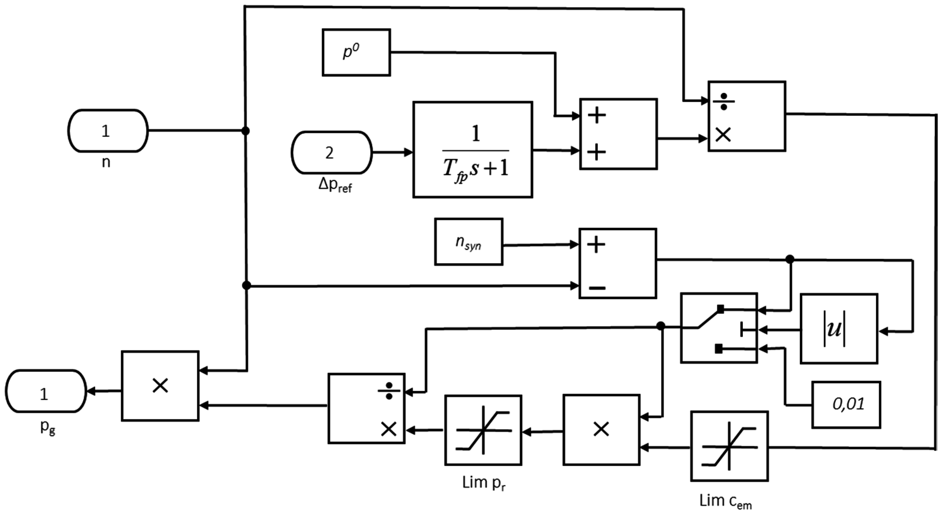
3.7. Doubly Fed Induction Generator Electrical Model

The electromagnetic torque is assumed to be controlled by the rotor-side inverter [23,24] in an instantaneous manner, comparing to the dynamics studied in the paper. In the “DFIG electrical model” block the electromagnetic torque, c_em (p.u.) and the rotor power, p_r (p.u.) are calculated from the running speed, n and the required electric power, (p⁰ + Δp_ref) (Figure 5). If none of these values exceeds its corresponding upper limit, the electric power output matches exactly the required electric power; otherwise, the electric power output is conveniently limited. The power losses in the generator are neglected.

Figure 5. “DFIG electrical model” block. (T_fp (s) is the converter time constant and n_syn (p.u.) is the synchronous speed of the group). Doubly fed induction generators: DFIG.

Figure 5. “DFIG electrical model” block. (T_fp (s) is the converter time constant and n_syn (p.u.) is the synchronous speed of the group). Doubly fed induction generators: DFIG.

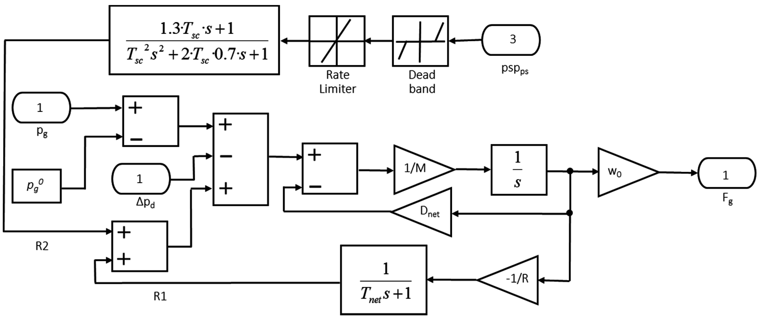
3.8. Power System

A single node inertial model has been used in this paper to represent the isolated power system. This assumption is accepted for the time scale of the dynamics analyzed in this work [25,26]. The changes in the system frequency are calculated from the unbalance between total generation and demand in Equation (12), in the “power system” block:

$$\frac{M}{{\mathsf{\omega }}^0}\frac{\text{d}{F}_{\text{g}}}{\text{d}t}=\left[\Delta p_{\text{g}}-\Delta p_{\text{d}}-D_{\text{net}}\frac{F_{\text{g}}}{{\mathsf{\omega }}^0}+R1+R2\right]$$

(12)

$$\frac{\text{d}R1}{\text{d}t}=\frac{1}{T_{\text{net}}}\left[-\frac{F_{\text{g}}}{{\mathsf{\omega }}^{0}R}-R1\right]$$

(13)

Wind and solar generators are supposed to be connected to the system through frequency converters and do not contribute to system inertia. The contribution of the thermal generation to the primary load-frequency control is represented by R1 (p.u.) in Equation (13) [27]. The contribution of the thermal generation to the secondary load-frequency control R2 (p.u.) is modelled through the transfer function proposed in [28], Figure 6. Although modern wind and solar generators could contribute to the load-frequency regulation, this contribution entails a cost: some energy will be lost [18]. Therefore, in this paper no contribution to frequency regulation from the wind and solar farms is assumed.

Figure 6. “Power system” block (T_sc (s) is the parameter of the transfer function used to model the secondary load frequency control of the synchronized thermal units).

Figure 6. “Power system” block (T_sc (s) is the parameter of the transfer function used to model the secondary load frequency control of the synchronized thermal units).

In expressions of Equations (12) and (13), Δp_d (p.u.) is the variation in the load demand at rated frequency, Δp_g (p.u.) is the variation in the electric power delivered to grid by the PSHP, M (s) is the equivalent mechanical inertia of the power system, R (p.u.) is the equivalent permanent droop of the synchronized thermal units, D_net (p.u./p.u.) the power system damping constant and T_net (s) is the time constant of the primary load-frequency control provided by the synchronized thermal unit.

3.9. Automatic Generation Control

In the Spanish insular power systems, an AGC system is in charge of eliminating the frequency deviations after the performance of the primary load-frequency control. In this paper, the AGC system is modelled in a similar way to [7]. The proportional coefficient in the control area K_f (MW/Hz) is calculated using the recommendations of [29]. The total regulation effort RR (p.u.), is proportional to the frequency deviation F_g in Equation (14). The regulation effort is distributed among the synchronized units as a function of the participation factors K_hp, K_ps, (p.u.) in Equations (15) and (16) [30]. In expressions of Equations (15) and (16), subscript hp refers to the PSHP and subscript ps refers to the power system; psp_hp (p.u.) is the increment in the power set-point signal sent by the AGC, psp_ps (p.u.) is the increment in the power set-point of the synchronized thermal units, T_hp (s) is the time constant of the AGC system for the PSHP and T_ps (s) is the time constant of the AGC system for the synchronized thermal units:

$$RR=-K_{\text{f}}\frac{F_{\text{g}}}{{\mathsf{\omega }}_{\text{0}}}$$

(14)

$$\frac{\text{d}\left(ps{p}_{\text{hp}}\right)}{\text{d}t}=\frac{K_{\text{hp}}}{T_{\text{hp}}}RR$$

(15)

$$\frac{\text{d}\left(ps{p}_{\text{ps}}\right)}{\text{d}t}=\frac{K_{\text{ps}}}{T_{\text{ps}}}RR$$

(16)

3.10. Model Numerical Values

In this section a summary of the main model magnitudes is presented. Table 1 contains the model base values. Table 2 lists the values of the model parameters. The parameters of the power system were properly calibrated in [7] from the system response during a load tripping event.

Table 2. Model parameter values.

Block	Parameter	Long/Short Penstock
Penstock	r	0.1363
	L	1350/300 m
	ap	1000 m/s
	Tw	4.14/0.92 s
	Te	1.35/0.30 s
Turbine-DFIG inertial model	Tm	6.00 s
Gross head	hc	1.250–1.068
Speed governor	δ	2.336/0.384
	Tr	8.65/4.60 s
Electrical model doubly fed induction generator (DFIG)	Tfp	0.5 s
	nsyn	1.0 p.u.
	cem,max, cem,min	1.2/0.0 p.u.
	pr,max, pr,min	0.15/−0.15
Power control	K	0.0531 p.u.
	Td	0.0191 s
	Tfnf	2 s
Power system	M	804 s
	R	0.0018 p.u.
	Dnet	0.5 p.u./p.u.
	Tnet	1 s
	Tsc	10 s
Automatic generation control (AGC)	Tu	100 s
	Tps	150 s
	Kf	575.04 MW/Hz
	Ku	0.15 p.u.
	Kps	0.85 p.u.

Table 2. Model parameter values.

Block	Parameter	Long/Short Penstock
Penstock	r	0.1363
	L	1350/300 m
	ap	1000 m/s
	Tw	4.14/0.92 s
	Te	1.35/0.30 s
Turbine-DFIG inertial model	Tm	6.00 s
Gross head	hc	1.250–1.068
Speed governor	δ	2.336/0.384
	Tr	8.65/4.60 s
Electrical model doubly fed induction generator (DFIG)	Tfp	0.5 s
	nsyn	1.0 p.u.
	cem,max, cem,min	1.2/0.0 p.u.
	pr,max, pr,min	0.15/−0.15
Power control	K	0.0531 p.u.
	Td	0.0191 s
	Tfnf	2 s
Power system	M	804 s
	R	0.0018 p.u.
	Dnet	0.5 p.u./p.u.
	Tnet	1 s
	Tsc	10 s
Automatic generation control (AGC)	Tu	100 s
	Tps	150 s
	Kf	575.04 MW/Hz
	Ku	0.15 p.u.
	Kps	0.85 p.u.

Governor PI gains have been adjusted by using two different tuning criteria. On one hand, for the long penstock configuration, the criterion proposed in [18] has been used. This criterion considers the elasticity of both water and penstock, as it is required in long penstocks [31]. On the other hand, for the short penstock configuration the tuning criterion proposed in [32] is used. This criterion is one of the most used ones for isolated power plants and usually yields moderate oscillations in the wicket gates position. As can be seen in Table 2, the head loss in the penstock, expressed in per unit values with respect to the base head, is assumed to be identical for both configurations. The possible differences that might exist between the two configurations are expected not to appreciably affect the parameters used to evaluate and compare the speed control strategies analyzed in the paper.

4. Control Strategies for the Speed Control Loop

As it was above-mentioned, different control strategies have been studied for the speed control loop of the pumped-storage unit. The studied control strategies are summarized below. It is important to mention that the option of bypassing the converter is not considered in the paper:

Strategy A (n^ref = n^fix). The reference speed n^ref is kept constant during the whole simulation. Two different values have been adopted: the speed (n^fix = 1.051) at which the unit provides the rated power (p_g = p_t = 1.0) with the best efficiency and an intermediate gross head (h_c = 1.131); and the speed (n^fix = 1.088) at which the unit provides an intermediate power (p_g = p_t = 0.7) with the best efficiency and the same gross head. The first speed corresponds to the design or rated conditions, whereas the second one corresponds to an intermediate value of power that maximizes the up and down power reserve and that will likely be the most frequent steady-state operating point.

Strategy B (n^ref = n^opt,fix). The reference speed is optimum for the initial operating point (h_c⁰ and p⁰) and is kept constant during the simulation.

Strategy C (n^ref = n^opt,var). The reference speed varies throughout the simulation as a function of the operating point (h_c and p_t). The reference speed changes every T_n seconds (hereinafter referred to as update period).

5. Simulations

The above-described strategies have been evaluated in terms of the amount of water discharged Vol, and the wicket gates fatigue, while providing load-frequency control, considering different initial operating points and penstock lengths, as well as different update periods for the strategy C. The wicket gates fatigue has been measured as the number of changes in the sign of the first derivative of the wicket gates position, zvar. Therefore, in each simulation zvar is an integer value but in some tables it is expressed as a decimal number resulting from the averaging of the multiple simulations. Table 3 summarizes the initial operating points considered in the simulations. 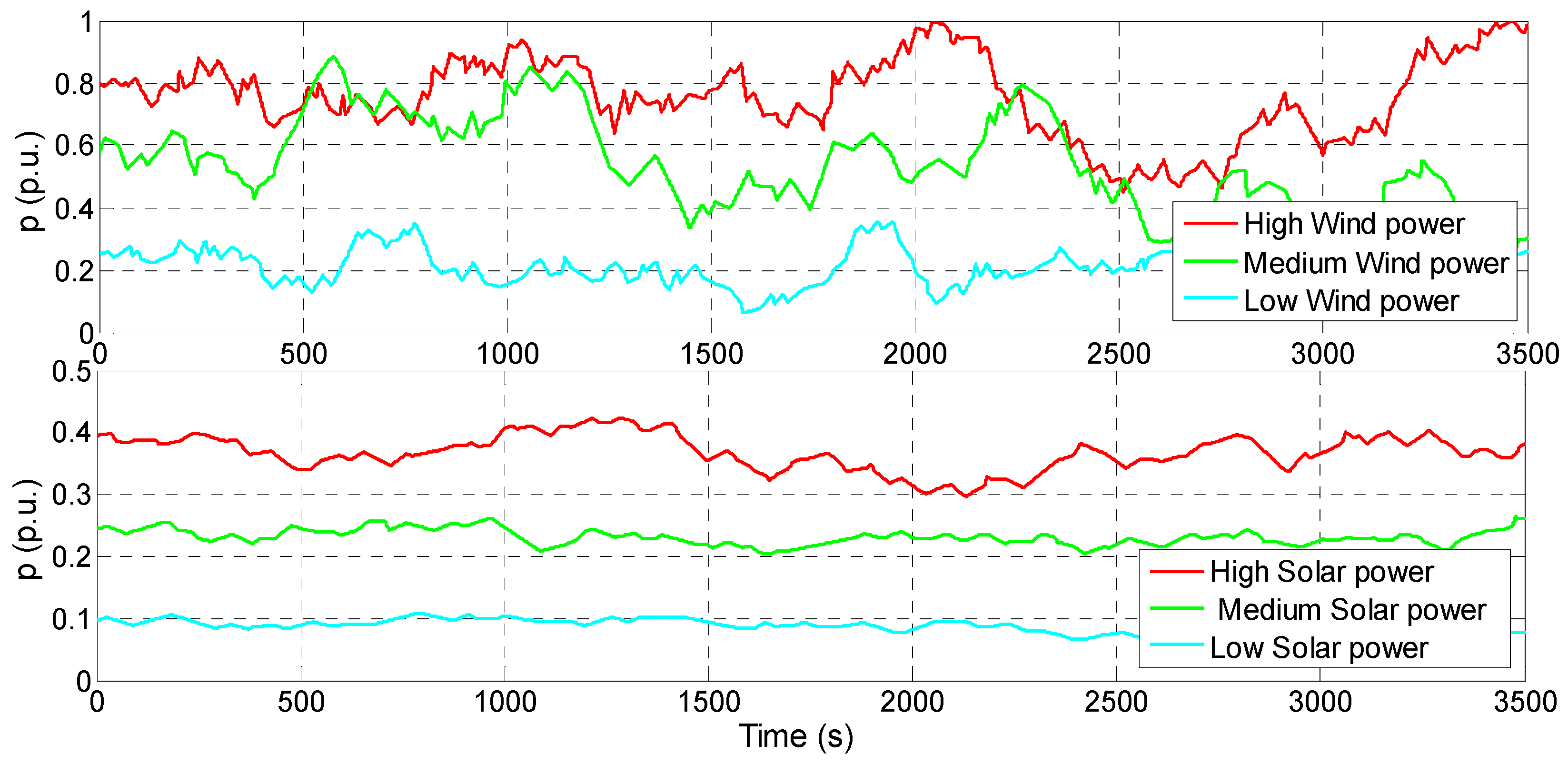The initial operating points have been superimposed on the pump-turbine hill chart in Figure 4. The dynamic response of the PSHP has been simulated with each strategy, initial operating point, and update periods for strategy C, in nine different scenarios of wind and solar power.

These scenarios have been built by combining the wind and solar photovoltaic power records presented in [33], conveniently scaled to the installed wind and photovoltaic power in the system under study. Said power records are shown in Figure 7, expressed in per unit values with respect to the maximum wind and solar power in the system analyzed in [33]. The nine scenarios are characterized in Table 4, in terms of the wind and solar power output level.

Table 3. Initial values for each operating point considered in this study. eff is the turbine efficiency. Superscripts 0 indicate initial conditions.

hc0	p0	nfix/nopt,fix	q0	h0	z0	eff0
1.068	0.8	1.051	0.777	1.027	0.574	0.918
		1.088	0.781	1.027	0.587	0.912
		1.017	0.779	1.027	0.566	0.920
	0.7	1.051	0.694	1.035	0.503	0.902
		1.088	0.698	1.035	0.516	0.899
		1.040	0.691	1.036	0.498	0.902
	0.6	1.051	0.601	1.044	0.428	0.881
		1.088	0.602	1.043	0.439	0.878
		1.045	0.601	1.044	0.427	0.881
1.131	0.8	1.051	0.731	1.123	0.498	0.904
		1.088	0.722	1.123	0.501	0.903
		1.081	0.728	1.123	0.504	0.904
	0.7	1.051	0.646	1.131	0.431	0.883
		1.088	0.644	1.131	0.440	0.885
		1.088	0.644	1.131	0.440	0.885
	0.6	1.051	0.562	1.137	0.364	0.859
		1.088	0.563	1.137	0.376	0.862
		1.096	0.561	1.138	0.376	0.862
1.250	0.8	1.051	0.689	1.218	0.433	0.882
		1.088	0.684	1.218	0.440	0.886
		1.130	0.681	1.218	0.449	0.888
	0.7	1.051	0.613	1.224	0.375	0.861
		1.088	0.608	1.225	0.382	0.866
		1.135	0.605	1.225	0.393	0.869
	0.6	1.051	0.536	1.230	0.317	0.835
		1.088	0.534	1.230	0.325	0.840
		1.143	0.533	1.230	0.338	0.844

Table 3. Initial values for each operating point considered in this study. eff is the turbine efficiency. Superscripts 0 indicate initial conditions.

hc0	p0	nfix/nopt,fix	q0	h0	z0	eff0
1.068	0.8	1.051	0.777	1.027	0.574	0.918
		1.088	0.781	1.027	0.587	0.912
		1.017	0.779	1.027	0.566	0.920
	0.7	1.051	0.694	1.035	0.503	0.902
		1.088	0.698	1.035	0.516	0.899
		1.040	0.691	1.036	0.498	0.902
	0.6	1.051	0.601	1.044	0.428	0.881
		1.088	0.602	1.043	0.439	0.878
		1.045	0.601	1.044	0.427	0.881
1.131	0.8	1.051	0.731	1.123	0.498	0.904
		1.088	0.722	1.123	0.501	0.903
		1.081	0.728	1.123	0.504	0.904
	0.7	1.051	0.646	1.131	0.431	0.883
		1.088	0.644	1.131	0.440	0.885
		1.088	0.644	1.131	0.440	0.885
	0.6	1.051	0.562	1.137	0.364	0.859
		1.088	0.563	1.137	0.376	0.862
		1.096	0.561	1.138	0.376	0.862
1.250	0.8	1.051	0.689	1.218	0.433	0.882
		1.088	0.684	1.218	0.440	0.886
		1.130	0.681	1.218	0.449	0.888
	0.7	1.051	0.613	1.224	0.375	0.861
		1.088	0.608	1.225	0.382	0.866
		1.135	0.605	1.225	0.393	0.869
	0.6	1.051	0.536	1.230	0.317	0.835
		1.088	0.534	1.230	0.325	0.840
		1.143	0.533	1.230	0.338	0.844

Figure 7. Wind and solar power records taken from [31].

Figure 7. Wind and solar power records taken from [31].

Table 4. Wind and solar power scenarios analyzed in the paper. H = high, M = medium, L = low.

Scenario	1	2	3	4	5	6	7	8	9
Wind power output	H	H	H	M	M	M	L	L	L
Solar power output	H	M	L	H	M	L	H	M	L

Table 4. Wind and solar power scenarios analyzed in the paper. H = high, M = medium, L = low.

Scenario	1	2	3	4	5	6	7	8	9
Wind power output	H	H	H	M	M	M	L	L	L
Solar power output	H	M	L	H	M	L	H	M	L

6. Simulation Results

The main results obtained in this study are discussed in the following subsections. The numerical values presented in the following tables and figures are the average values across the nine considered scenarios.

6.1. Update Period

Table 5 and Table 6 show the results obtained for different update periods (strategy C) and compare these results with those obtained with strategies A and B. The results corresponding to the strategy A are used as a basis for the comparison. The results included in the tables are the average values across all considered initial operation points, (p⁰ = 0.6, 0.7, 0.8 and h_c⁰ = 1.068, 1.131, 1.250). As can be seen in Table 5, for both long and short penstock configurations, there is an update period which minimizes Vol and another which minimizes zvar.

Table 5. Vol and zvar with the three control strategies and different update periods for the strategy C, n^fix = 1.0508 p.u.

Strategy		Long	Short	Long	Short
Strategy	nref	Vol (m3)		zvar
A	nfix	23,850.1	23,920.0	80.8	113.0
Strategy	Tn-nopt,var	ΔVol (%)		Δzvar (%)
C	10 s	−0.2794	−0.2790	275.6	420.6
	30 s	−0.2799	−0.2791	163.9	219.4
	60 s	−0.2807	−0.2789	96.27	132.23
	120 s	−0.2815	−0.2781	46.03	73.24
	300 s	−0.2794	−0.2740	14.20	28.42
	600 s	−0.2739	−0.2679	5.457	12.79
	900 s	−0.2753	−0.2705	2.391	8.683
	1200 s	−0.2637	−0.2593	−0.4596	3.809
	1500 s	−0.2734	−0.2706	2.140	6.857
B	nopt,fix	−0.2620	−0.2604	−4.262	−1.533

Table 5. Vol and zvar with the three control strategies and different update periods for the strategy C, n^fix = 1.0508 p.u.

Strategy		Long	Short	Long	Short
Strategy	nref	Vol (m3)		zvar
A	nfix	23,850.1	23,920.0	80.8	113.0
Strategy	Tn-nopt,var	ΔVol (%)		Δzvar (%)
C	10 s	−0.2794	−0.2790	275.6	420.6
	30 s	−0.2799	−0.2791	163.9	219.4
	60 s	−0.2807	−0.2789	96.27	132.23
	120 s	−0.2815	−0.2781	46.03	73.24
	300 s	−0.2794	−0.2740	14.20	28.42
	600 s	−0.2739	−0.2679	5.457	12.79
	900 s	−0.2753	−0.2705	2.391	8.683
	1200 s	−0.2637	−0.2593	−0.4596	3.809
	1500 s	−0.2734	−0.2706	2.140	6.857
B	nopt,fix	−0.2620	−0.2604	−4.262	−1.533

Table 6. Vol and zvar with the three control strategies and different update periods for the strategy C, n^fix = 1.0882 p.u.

Strategy		Long	Short	Long	Short
Strategy	nref	Vol (m3)		zvar
A	nfix	23,884.3	23,884.5	70.7	109.8
Strategy	Tn-nopt,var	ΔVol (%)		Δzvar (%)
C	10 s	−0.1892	−0.2011	280.7	435.9
	30 s	−0.1898	−0.2290	176.4	227.0
	60 s	−0.1907	−0.2009	106.9	139.1
	120 s	−0.1916	−0.2001	54.09	78.30
	300 s	−0.1896	−0.1960	21.17	32.16
	600 s	−0.1842	−0.1900	12.66	16.05
	900 s	−0.1855	−0.1926	9.277	11.83
	1200 s	−0.1736	−0.2092	6.806	6.235
	1500 s	−0.1832	−0.1926	9.484	9.947
B	nopt,fix	−0.1715	−0.2103	2.923	0.7704

Table 6. Vol and zvar with the three control strategies and different update periods for the strategy C, n^fix = 1.0882 p.u.

Strategy		Long	Short	Long	Short
Strategy	nref	Vol (m3)		zvar
A	nfix	23,884.3	23,884.5	70.7	109.8
Strategy	Tn-nopt,var	ΔVol (%)		Δzvar (%)
C	10 s	−0.1892	−0.2011	280.7	435.9
	30 s	−0.1898	−0.2290	176.4	227.0
	60 s	−0.1907	−0.2009	106.9	139.1
	120 s	−0.1916	−0.2001	54.09	78.30
	300 s	−0.1896	−0.1960	21.17	32.16
	600 s	−0.1842	−0.1900	12.66	16.05
	900 s	−0.1855	−0.1926	9.277	11.83
	1200 s	−0.1736	−0.2092	6.806	6.235
	1500 s	−0.1832	−0.1926	9.484	9.947
B	nopt,fix	−0.1715	−0.2103	2.923	0.7704

The results shown in Table 5 and Table 6 confirm that the strategy C allows reducing the amount of water discharged while providing load-frequency control, with respect to the strategies A and B. However, this benefit comes at the expense of an increase in the wicket gates fatigue, especially for the short penstock configuration. The strategy B yields a reduction in the amount of water discharged of a similar magnitude to that yielded by the strategy C, with a significantly lower wicket gates fatigue.

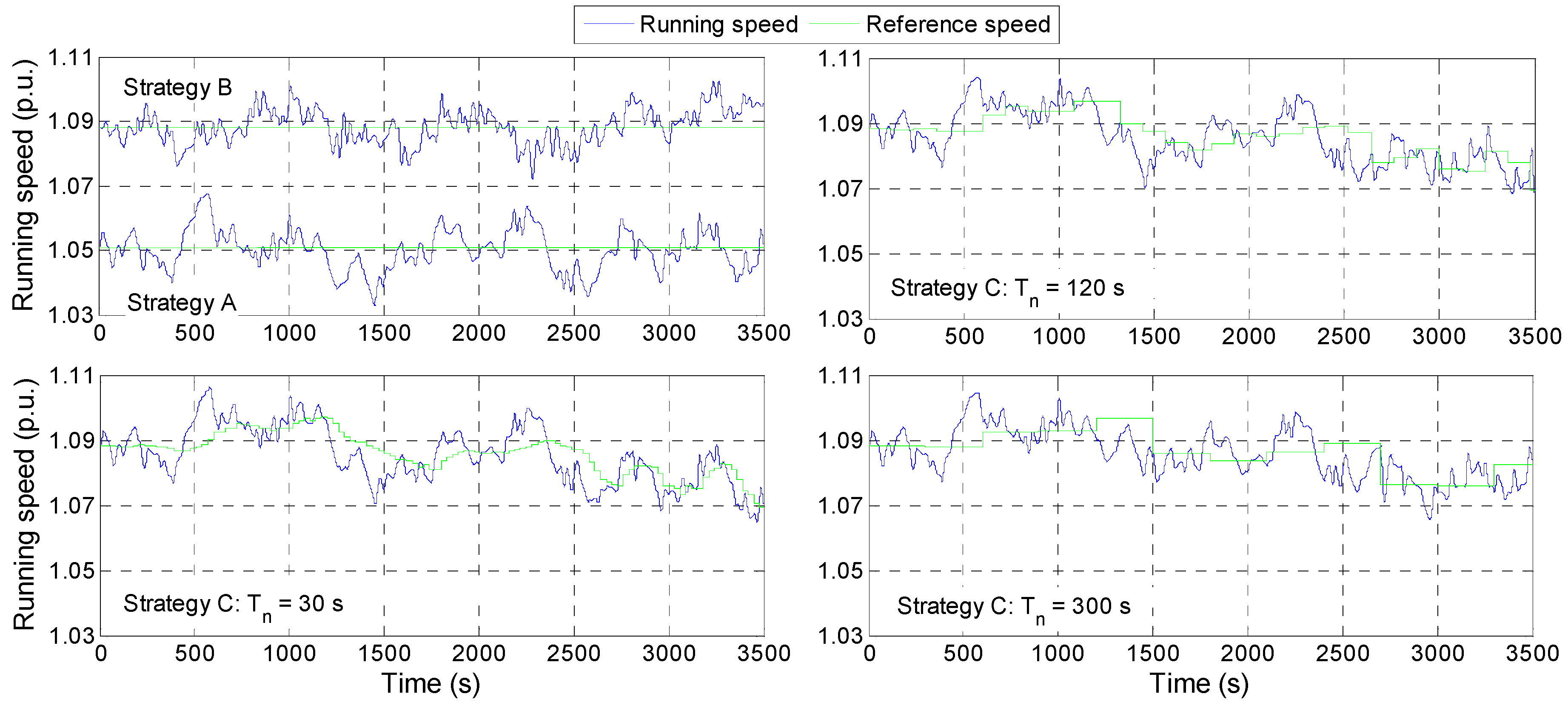
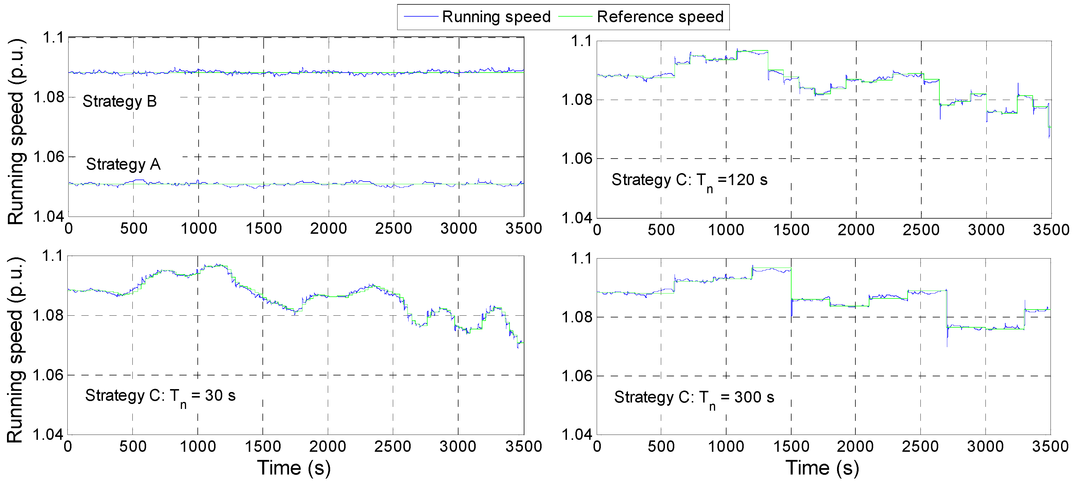
Figure 8 and Figure 9 show the running speed and the reference speed with the three control strategies for the long and short penstock configurations, in scenario 1 and with a specific initial operating point. By comparing Figure 8 and Figure 9 it is observed that the lower water inertia in the short penstock facilitates the governor to maintain the unit speed close to the reference speed albeit at the expense of a considerable increase in the wicket gates fatigue, as shown in Table 5 and Table 6.

Figure 8. Running speed and reference speed with the three strategies. Long penstock configuration, p⁰ = 0.7 p.u., h_c⁰ = 1.131 p.u., scenario 1.

Figure 8. Running speed and reference speed with the three strategies. Long penstock configuration, p⁰ = 0.7 p.u., h_c⁰ = 1.131 p.u., scenario 1.

Figure 9. Running speed and reference speed with the three strategies. Short penstock configuration, p⁰ = 0.7 p.u., h_c⁰ = 1.131 p.u., scenario 1.

Figure 9. Running speed and reference speed with the three strategies. Short penstock configuration, p⁰ = 0.7 p.u., h_c⁰ = 1.131 p.u., scenario 1.

6.2. Initial Power

Table 7 and Table 8 show the results obtained with the three control strategies for different initial powers delivered to the system by the PSHP. The results corresponding to the strategy A are used as a basis for the comparison. The results included in the Tables are the average values across the three initial considered gross heads. The update periods which give the least Vol and the least zvar in Table 5 and Table 6 have been used for the strategy C in this case.

On the one hand, the results shown in Table 7 and Table 8 confirm those discussed in Section 6.1: the strategy B yields a reduction in the amount of water discharged similar to that yielded by the strategy C, with a considerable reduction in the wicket gates fatigue. On the other hand, the results shown in these tables demonstrate that the water savings yielded by the strategies B and C slightly decrease as the initial power decreases; as can be seen in Figure 4, the efficiency barely changes with speed for the lowest initial power (p⁰ = 0.6).

Table 7. Vol and zvar with the three control strategies, and different initial pumped storage hydropower plants (PSHP) powers p⁰, n^fix = 1.0508 p.u.

p0	Strategy	nref	Vol/zvar/ ΔVol/Δzvar	Long Penstock Tn 120/1200 s	Short Penstock Tn 30/1200 s
0.8	A	nfix	Vol (m3)	26,825.2	26,846.5
			zvar	78.7	119.7
	B	nopt,fix	ΔVol (%)	−0.3592	−0.3554
			Δzvar (%)	−3.4901	−0.6819
	C	nopt,var	ΔVol (%)	−0.3869/−0.3589	−0.3839/−0.3532
			Δzvar (%)	45.51/0.1908	233.2/4.957
0.7	A	nfix	Vol (m3)	23,753.1	23,874.9
			zvar	89.0	113.6
	B	nopt.fix	ΔVol (%)	−0.2602	−0.2601
			Δzvar (%)	−3.7764	−1.986
	C	nopt,var	ΔVol (%)	−0.2794/−0.2633	−0.2769/−0.2597
			Δzvar (%)	51.98/0.7453	219.8/3.265
0.6	A	nfix	Vol (m3)	20,972.0	21,038.6
			zvar	74.7	105.7
	B	nopt,fix	ΔVol (%)	−0.1667	−0.4460
			Δzvar (%)	−5.5194	−1.930
	C	nopt,var	ΔVol (%)	−0.1782/−0.1689	−0.4569/−0.4455
			Δzvar (%)	40.60/−1.933	205.3/3.204

Table 7. Vol and zvar with the three control strategies, and different initial pumped storage hydropower plants (PSHP) powers p⁰, n^fix = 1.0508 p.u.

p0	Strategy	nref	Vol/zvar/ ΔVol/Δzvar	Long Penstock Tn 120/1200 s	Short Penstock Tn 30/1200 s
0.8	A	nfix	Vol (m3)	26,825.2	26,846.5
			zvar	78.7	119.7
	B	nopt,fix	ΔVol (%)	−0.3592	−0.3554
			Δzvar (%)	−3.4901	−0.6819
	C	nopt,var	ΔVol (%)	−0.3869/−0.3589	−0.3839/−0.3532
			Δzvar (%)	45.51/0.1908	233.2/4.957
0.7	A	nfix	Vol (m3)	23,753.1	23,874.9
			zvar	89.0	113.6
	B	nopt.fix	ΔVol (%)	−0.2602	−0.2601
			Δzvar (%)	−3.7764	−1.986
	C	nopt,var	ΔVol (%)	−0.2794/−0.2633	−0.2769/−0.2597
			Δzvar (%)	51.98/0.7453	219.8/3.265
0.6	A	nfix	Vol (m3)	20,972.0	21,038.6
			zvar	74.7	105.7
	B	nopt,fix	ΔVol (%)	−0.1667	−0.4460
			Δzvar (%)	−5.5194	−1.930
	C	nopt,var	ΔVol (%)	−0.1782/−0.1689	−0.4569/−0.4455
			Δzvar (%)	40.60/−1.933	205.3/3.204

Table 8. Vol and zvar with the three control strategies, and different initial PSHP powers p⁰, n^fix = 1.0882 p.u.

p0	Strategy	nref	Vol/zvar/ ΔVol/Δzvar	Long Penstock Tn 120/1200 s	Short Penstock Tn 30/1200 s
0.8	A	nfix	Vol (m3)	26,819.2	26,821.9
			zvar	70.3	115.2
	B	nopt,fix	ΔVol (%)	−0.2310	−0.3348
			Δzvar (%)	7.158	1.7152
	C	nopt,var	ΔVol (%)	−0.2587/−0.2307	−0.3632/0.3326
			Δzvar (%)	61.64/10.78	241.30/7.48
0.7	A	nfix	Vol (m3)	23,870.2	23,869.2
			zvar	71.2	110.2
	B	nopt,fix	ΔVol (%)	−0.2245	−0.2319
			Δzvar (%)	1.920	1.084
	C	nopt,var	ΔVol (%)	−0.2455/−0.2289	−0.2486/−0.2314
			Δzvar (%)	52.17/6.13	229.92/6.50
0.6	A	nfix	Vol (m3)	20,963.4	20,962.5
			zvar	70.6	104.1
	B	nopt,fix	ΔVol (%)	−0.0590	−0.0643
			Δzvar (%)	−0.308	−0.4879
	C	nopt,var	ΔVol (%)	−0.0705/−0.0612	−0.0751/−0.0638
			Δzvar (%)	48.46/3.505	209.67/4.724

Table 8. Vol and zvar with the three control strategies, and different initial PSHP powers p⁰, n^fix = 1.0882 p.u.

p0	Strategy	nref	Vol/zvar/ ΔVol/Δzvar	Long Penstock Tn 120/1200 s	Short Penstock Tn 30/1200 s
0.8	A	nfix	Vol (m3)	26,819.2	26,821.9
			zvar	70.3	115.2
	B	nopt,fix	ΔVol (%)	−0.2310	−0.3348
			Δzvar (%)	7.158	1.7152
	C	nopt,var	ΔVol (%)	−0.2587/−0.2307	−0.3632/0.3326
			Δzvar (%)	61.64/10.78	241.30/7.48
0.7	A	nfix	Vol (m3)	23,870.2	23,869.2
			zvar	71.2	110.2
	B	nopt,fix	ΔVol (%)	−0.2245	−0.2319
			Δzvar (%)	1.920	1.084
	C	nopt,var	ΔVol (%)	−0.2455/−0.2289	−0.2486/−0.2314
			Δzvar (%)	52.17/6.13	229.92/6.50
0.6	A	nfix	Vol (m3)	20,963.4	20,962.5
			zvar	70.6	104.1
	B	nopt,fix	ΔVol (%)	−0.0590	−0.0643
			Δzvar (%)	−0.308	−0.4879
	C	nopt,var	ΔVol (%)	−0.0705/−0.0612	−0.0751/−0.0638
			Δzvar (%)	48.46/3.505	209.67/4.724

6.3. Gross Head

The storage capacity of the upper reservoir is small and therefore both the water level and the gross head h_c are expected to vary frequently. Table 9 and Table 10 show the results obtained with the three control strategies for different initial gross heads. The results corresponding to the strategy A are used as a basis for the comparison. The results included in the Tables are the average values across the three initial considered powers (p⁰ = 0.6, 0.7 and 0.8). The update periods which give the least Vol and the least zvar in Table 5 and Table 6 have been used in this case.

Table 9. Vol and zvar with the three control strategies, and different initial gross heads h_c⁰, n^fix = 1.0508 p.u.

hc0	Strategy	nref	Vol/zvar/ ΔVol/Δzvar	Long Penstock Tn 120/1200 s	Short Penstock Tn 30/1200 s
1.068	A	nfix	Vol (m3)	25,386.3	25,505.4
			zvar	68.2	112.8
	B	nopt,fix	ΔVol (%)	−0.0606	−0.0693
			Δzvar (%)	6.324	2.596
	C	nopt,var	ΔVol (%)	−0.0934/−0.0618	−0.1016/−0.0668
			Δzvar (%)	61.53/10.29	237.0/8.359
1.131	A	nfix	Vol (m3)	23,790.5	23,789.6
			zvar	89.7	114.0
	B	nopt,fix	ΔVol (%)	−0.2164	−0.2185
			Δzvar (%)	−4.969	−2.260
	C	nopt,var	ΔVol (%)	−0.2333/−0.2187	−0.2351/−0.2189
			Δzvar (%)	49.97/−0.6262	220.8/3.145
1.250	A	nfix	Vol (m3)	22,373.5	22,408.9
			zvar	84.5	112.3
	B	nopt,fix	ΔVol (%)	−0.5091	−0.4934
			Δzvar (%)	−14.14	−4.934
	C	nopt,var	ΔVol (%)	−0.5179/−0.5106	−0.5006/−0.4923
			Δzvar (%)	26.58/−11.05	200.5/−0.0772

Table 9. Vol and zvar with the three control strategies, and different initial gross heads h_c⁰, n^fix = 1.0508 p.u.

hc0	Strategy	nref	Vol/zvar/ ΔVol/Δzvar	Long Penstock Tn 120/1200 s	Short Penstock Tn 30/1200 s
1.068	A	nfix	Vol (m3)	25,386.3	25,505.4
			zvar	68.2	112.8
	B	nopt,fix	ΔVol (%)	−0.0606	−0.0693
			Δzvar (%)	6.324	2.596
	C	nopt,var	ΔVol (%)	−0.0934/−0.0618	−0.1016/−0.0668
			Δzvar (%)	61.53/10.29	237.0/8.359
1.131	A	nfix	Vol (m3)	23,790.5	23,789.6
			zvar	89.7	114.0
	B	nopt,fix	ΔVol (%)	−0.2164	−0.2185
			Δzvar (%)	−4.969	−2.260
	C	nopt,var	ΔVol (%)	−0.2333/−0.2187	−0.2351/−0.2189
			Δzvar (%)	49.97/−0.6262	220.8/3.145
1.250	A	nfix	Vol (m3)	22,373.5	22,408.9
			zvar	84.5	112.3
	B	nopt,fix	ΔVol (%)	−0.5091	−0.4934
			Δzvar (%)	−14.14	−4.934
	C	nopt,var	ΔVol (%)	−0.5179/−0.5106	−0.5006/−0.4923
			Δzvar (%)	26.58/−11.05	200.5/−0.0772

Table 10. Vol and zvar with the three control strategies, and different initial gross heads h_c⁰, n^fix = 1.0882 p.u.

hc0	Strategy	nref	Vol/zvar/ ΔVol/Δzvar	Long Penstock Tn 120/1200 s	Short Penstock Tn 30/1200 s
1.068	A	nfix	Vol (m3)	25,547.1	25,547.3
			z var	65.1	110.0
	B	nopt,fix	ΔVol (%)	−0.2122	−0.2256
			Δzvar (%)	11.476	5.224
	C	nopt,var	ΔVol (%)	−0.2449/−0.2134	−0.2578/−0.2231
			Δzvar (%)	69.40/15.60	245.66/11.13
1.131	A	nfix	Vol (m3)	23,740.1	23,737.8
			z var	72.1	111.0
	B	nopt,fix	ΔVol (%)	−0.0045	−0.0882
			Δzvar (%)	0.628	−1.344
	C	nopt,var	ΔVol (%)	−0.0232/−0.0081	−0.1049/−0.0887
			Δzvar (%)	50.17/4.671	223.75/4.111
1.250	A	nfix	Vol (m3)	22,365.6	22,368.4
			z var	74.9	108.5
	B	nopt,fix	ΔVol (%)	−0.2978	−0.3171
			Δzvar (%)	−3.333	−1.568
	C	nopt,var	ΔVol (%)	−0.3066/−0.2993	−0.3243/−0.3160
			Δzvar (%)	42.70/0.149	211.48/3.46

Table 10. Vol and zvar with the three control strategies, and different initial gross heads h_c⁰, n^fix = 1.0882 p.u.

hc0	Strategy	nref	Vol/zvar/ ΔVol/Δzvar	Long Penstock Tn 120/1200 s	Short Penstock Tn 30/1200 s
1.068	A	nfix	Vol (m3)	25,547.1	25,547.3
			z var	65.1	110.0
	B	nopt,fix	ΔVol (%)	−0.2122	−0.2256
			Δzvar (%)	11.476	5.224
	C	nopt,var	ΔVol (%)	−0.2449/−0.2134	−0.2578/−0.2231
			Δzvar (%)	69.40/15.60	245.66/11.13
1.131	A	nfix	Vol (m3)	23,740.1	23,737.8
			z var	72.1	111.0
	B	nopt,fix	ΔVol (%)	−0.0045	−0.0882
			Δzvar (%)	0.628	−1.344
	C	nopt,var	ΔVol (%)	−0.0232/−0.0081	−0.1049/−0.0887
			Δzvar (%)	50.17/4.671	223.75/4.111
1.250	A	nfix	Vol (m3)	22,365.6	22,368.4
			z var	74.9	108.5
	B	nopt,fix	ΔVol (%)	−0.2978	−0.3171
			Δzvar (%)	−3.333	−1.568
	C	nopt,var	ΔVol (%)	−0.3066/−0.2993	−0.3243/−0.3160
			Δzvar (%)	42.70/0.149	211.48/3.46

As in the previous case, the water savings yielded by the strategies B and C are of a similar magnitude, whereas the wicket gates fatigue is notably smaller with strategy B. However, the water savings vary as a function of the initial gross head to a larger extent than as a function of the initial PSHP power. As can be seen in Table 9, the higher the initial gross head, the larger the water savings when n^fix = 1.0508 p.u. In turn, as can be seen in Table 10, when n^fix = 1.088 p.u, the further the initial gross head is from the most frequent gross head (h_c = 1.131 p.u.), the larger the water savings. Both results can be justified from Figure 4. As can be seen in said figure, when n^fix = 1.051, the higher the gross head (or the lower the unit speed n₁₁), the further the initial operating points are from the maximum efficiency curve, and therefore the larger the room for improving the efficiency by varying the running speed. In turn, when n^fix = 1.088 p.u, the initial operating points corresponding to the most frequent gross head (referred to as medium gross head in the figure) are very close to the maximum efficiency curve, and thus, the room for improving the efficiency by varying the running speed increases as the initial gross head separates from the most frequent gross head.

7. Conclusions

This paper analyses three different control strategies for the speed-control loop of a PSHP equipped with a pump-turbine and a DFIG when it operates in generating mode. The PSHP is connected to a small isolated power system with thermal, wind and solar generation, and which provides load-frequency control under the orders of an AGC system. The analyzed control strategies differ from each other in the way the reference speed is determined and in the frequency with which the reference speed is updated. In strategy A the reference speed is constant. Two different reference speeds have been considered for this strategy: those which maximize the efficiency for the rated operating conditions and for the most frequent operating point. In strategy B, the reference speed is constant and is optimum for the initial operating point. And in strategy C, the reference speed varies as a function of the actual operating point and is updated every T_n seconds. The control strategies have been evaluated in terms of the amount of water discharged, and the wicket gates fatigue, while providing load-frequency control. Another feasible control strategy not considered in this work would be to optimize the wicket gate fatigue instead of the efficiency or to perform a multi-objective optimization. The wicket gates fatigue has been measured as the number of changes in the sign of the first derivative of the wicket gates position. Different T_n (update periods) have been analyzed for strategy C. For these purposes, several simulations have been performed.

The results of the simulations demonstrate that with respect to strategy A, strategies B and C allow reducing the amount of water discharged while providing load-frequency control. In general, strategy C yields higher water savings than strategy B, albeit at the expense of a significant increase in the wicket gates fatigue. Strategy B yields water savings of a similar magnitude to those yielded by strategy C, and a wicket gates fatigue lower in all cases than that of strategy C, and in most cases than that of strategy A.

The influence of the penstock length, and the initial operating point on the water usage and the wicket gates fatigue has also been analyzed. The results of the simulations show that neither the penstock length nor the initial operating point has a significant influence on the selection of the best control strategy. In general, the longer the penstock the lower the wicket gates fatigue with the three control strategies, what can be expected to a certain extent, due to the higher water inertia. The penstock length does have a considerable influence on the optimum update period for strategy C.

An interesting practical conclusion can be drawn from the results obtained in the paper. According to these results, the best way to implement variable speed in a pump-turbine unit that operates in generating mode and that provides load-frequency control, would be to update the reference speed according to the power generation schedule and keep it constant within each scheduling period (typically 1 h).

Finally, as a future line of work it would be interesting to carry out a similar study with other pump-turbines of different specific speeds. Future studies should also consider different PI tuning criteria as well as the possibility to find a trade-off solution between the hydraulic efficiency and the wicket gates fatigue by means of a multi-objective approach. Additionally, the benefits of variable speed operation from the point of view of the Transmission System Operator (TSO) should be also analyzed.

References

- Eurelectric. Hydro in Europe: Powering Renewables, Full Report; the Union of the Electricity Industry—EURELECTRIC: Brussels, Belgium, 2011; Available online: http://www.eurelectric.org/media/26690/hydro_report_final-2011-160-0011-01-e.pdf (accessed on 12 December 2014).
- Anagnostopoulos, J.; Papantonis, D. Simulation and size of a pumped-storage power plant for the recovery of wind-farms rejected energy. Renew. Energy 2008, 33, 1685–1694. [Google Scholar] [CrossRef]
- Kaldellis, J.; Kavadias, K. Optimal wind-hydro solution for Aegean Sea islands’ electricity-demand fulfilment. Appl. Energy 2001, 70, 333–354. [Google Scholar] [CrossRef]
- Kaldellis, J.; Kavadias, K.; Christinakis, E. Evaluation of the wind-hydro energy solution for remote islands. Energy Convers. Manag. 2001, 42, 1105–1120. [Google Scholar] [CrossRef]
- Ma, T.; Yang, H.; Lu, L.; Peng, J. Technical feasibility study on a standalone hybrid solar-wind system with pumped hydro storage for a remote island in Hong Kong. Renew. Energy 2014, 69, 7–15. [Google Scholar] [CrossRef]
- Suul, J.A.; Uhlen, K.; Undeland, T. Wind power integration in isolated grids enabled by variable speed pumped storage hydropower plant. In Proceedings of the 2008 IEEE International Conference on Sustainable Energy Technologies (ICSET), Singapore, 24–27 November 2008.
- Pérez-Díaz, J.I.; Sarasúa, J.I.; Wilhelmi, J.R. Contribution of a hydraulic short-circuit pumped-storage power plant to the load-frequency regulation of an isolated power system. Int. J. Electr. Power Energy Syst. 2014, 62, 199–211. [Google Scholar] [CrossRef]
- Quintero, J.; Vittal, V.; Heydt, G.T.; Zhang, H. The impact of increased penetration of converter control-based generators on power system modes of oscillation. IEEE Trans. Power Syst. 2014, 29, 2248–2256. [Google Scholar] [CrossRef]
- Boukhezzar, B.; Siguerdidjane, H. Nonlinear control with wind estimation of a DFIG variable speed wind turbine for power capture optimization. Energy Convers. Manag. 2009, 50, 885–892. [Google Scholar] [CrossRef]
- Kopf, E.; Brausewetter, S. Control strategies for variable speed machines-design and optimization criteria. In Proceedings of the 2005 Hydro Conference, Villach, Austria, 17–20 October 2005.
- Erlich, I.; Bachmann, U. Dynamic behavior of variable speed pump storage units in the German electric power system. In Proceedings of the 2002 IFAC Triennial World Congress, Barcelona, Spain, 21–26 July 2002.
- Lung, J.-K.; Lu, Y.; Hung, W.-L.; Kao, W.-S. Modeling and dynamic simulations of doubly fed adjustable-speed pumped storage units. IEEE Trans. Energy Convers. 2007, 22, 250–258. [Google Scholar] [CrossRef]
- Nicolet, C.; Pannatier, Y.; Kawkabani, B.; Schwery, A.; Avellan, F.; Simond, J.-J. Benefits of variable speed pumped storage units in mixed islanded power network during transient operation. In Proceedings of the 2009 Hydro Conference, Lyon, France, 26–28 October 2009.
- Pannatier, Y.; Kawkabani, B.; Nicolet, C.; Simond, J.-J.; Schwery, A.; Allenbach, P. Investigation of control strategies for variable-speed pump-turbine units by using a simplified model of the converters. IEEE Trans. Ind. Electr. 2010, 57, 3039–3049. [Google Scholar] [CrossRef]
- Chaudhry, M.H. Applied Hydraulic Transients; Van Nostrand Reinhold Inc.: New York, NY, USA, 1987. [Google Scholar]
- Pérez-Díaz, J.I.; Wilhelmi, J.R.; Galaso, I.; Fraile-Ardanuy, J.; Sánchez, J.A.; Castañeda, O.; Sarasúa, J.I. Dynamic response of hydro power plants to load variations for providing secondary regulation reserves considering elastic water column effects. Energy 2012, 1, 159–163. [Google Scholar]
- Sarasúa, J.; Elías, P.; Martínez-Lucas, G.; Pérez-Diaz, J.; Wilhelmi, J.; Sánchez, J. Stability analysis of a run-of-river diversion hydropower plant with surge tank and spillway in the head pond. Sci. World J. 2014, 2014. [Google Scholar] [CrossRef] [PubMed]
- Martínez-Lucas, G.; Sarasúa, J.I.; Sánchez, J.Á.; Wilhemi, J.R. Power-frequency control of hydropower plants with long penstocks in isolated systems with wind generation. Renew. Energy 2015, 83, 245–255. [Google Scholar] [CrossRef]
- Carravetta, A.; Fecarotta, O.; Martino, R.; Antipodi, L. Pat efficiency variation with design parameters. Procedia Eng. 2014, 70, 285–291. [Google Scholar] [CrossRef]
- Suul, J.A.; Uhlen, K.; Undeland, T. Variable speed pumped storage hydropower for integration of wind energy in isolated grids-case description and control strategies. In Proceedings of the Nordic Workshop on Power and Industrial Electronics (NORPIE), Espoo, Finland, 9–11 June 2008.
- Morren, J.; Pierik, J.; de Haan, S.W.H. Inertial response of variable speed wind turbines. Electr. Power Syst. Res. 2006, 76, 980–987. [Google Scholar] [CrossRef]
- Margaris, I.D.; Papathanassiou, S.A.; Hatziargiriou, N.D.; Hansen, A.D.; Sorensen, P. Frequency control in autonomous power systems with high wind power penetration. IEEE Trans. Sustain. Energy 2012, 3, 189–199. [Google Scholar] [CrossRef]
- Machowski, J.; Bialek, J.W.; Bumby, J.R. Power System Dynamics: Stability and Control, 2nd ed.; John Wiley & Sons Limited: New York, NY, USA, 2008. [Google Scholar]
- Rodríguez, J.M.; Fernández, J.L.; Beato, D.; Iturbe, R.; Usaola, J.; Ledesma, P.; Wilhelmi, J.R. Incidence on power system dynamics of high penetration of fixed speed and doubly fed wind energy systems: Study of the Spanish case. IEEE Trans. Power Syst. 2002, 17, 1089–1095. [Google Scholar] [CrossRef]
- Grenier, M.-E.; Lefebvre, D.; van Cutsen, T. Quasi steady-state models for long-term voltage and frequency dynamics simulation. In Proceedings of the 2005 IEEE Russia Power Tech, St. Petersburg, Russia, 27–30 June 2005; pp. 1–8.
- Van Cutsen, T.; Grenier, M.-E.; Lefebvre, D. Combined detailed and quasi steady-state time simulations for large-disturbance analysis. Electr. Power Energy Syst. 2006, 28, 634–642. [Google Scholar] [CrossRef]
- Mansoor, S.P.; Jones, D.I.; Bradley, D.A.; Aris, F.C.; Jones, G.R. Reproducing oscillatory behaviour of a hydroelectric power station by computer simulation. Control Eng. Pract. 2000, 8, 1261–1272. [Google Scholar] [CrossRef]
- Egido, I.; Fernández-Bernal, F.; Rouco, L.; Porras, E.; Sáiz-Chicharro, A. Modeling of thermal generating units for automatic generation control purposes. IEEE Trans. Control Syst. Technol. 2004, 12, 205–210. [Google Scholar] [CrossRef]
- Union for the Co-ordination of Transmission of Electricity (UCTE). Continental Europe Operation Handbook. 2004. Available online: https://www.entsoe.eu/publications/system-operations-reports/operation-handbook (accessed on 23 December 2014).
- Wood, A.J.; Wollenberg, B.F. Power Generation Operation and Control, 2nd ed.; John Wiley & Sons Limited: New York, NY, USA, 1996. [Google Scholar]
- Clifton, L. Waterhammer and governor analysis. Int. Water Power Dam Constr. 1987, 39, 31–39. [Google Scholar]
- Kundur, P. Power System Stability and Control; Balu, N.J., Lauby, M.G., Eds.; McGraw-Hill: New York, NY, USA, 1994; Volume 7. [Google Scholar]
- Wada, K.; Yokoyama, A. Load frequency control using distributed batteries on the demand side with communication characteristics. In Proceedings of the 2012 3rd IEEE PES International Conference and Exhibition on Innovative Smart Grid Technologies (ISGT Europe), Berlin, Germany, 14–17 October 2012.
© 2015 by the authors; licensee MDPI, Basel, Switzerland. This article is an open access article distributed under the terms and conditions of the Creative Commons by Attribution (CC-BY) license (http://creativecommons.org/licenses/by/4.0/).