Optimal Subinterval Selection Approach for Power System Transient Stability Simulation

Abstract

Power system transient stability analysis requires an appropriate integration time step to avoid numerical instability as well as to reduce computational demands. For fast system dynamics, which vary more rapidly than what the time step covers, a fraction of the time step, called a subinterval, is used. However, the optimal value of this subinterval is not easily determined because the analysis of the system dynamics might be required. This selection is usually made from engineering experiences, and perhaps trial and error. This paper proposes an optimal subinterval selection approach for power system transient stability analysis, which is based on modal analysis using a single machine infinite bus (SMIB) system. Fast system dynamics are identified with the modal analysis and the SMIB system is used focusing on fast local modes. An appropriate subinterval time step from the proposed approach can reduce computational burden and achieve accurate simulation responses as well. The performance of the proposed method is demonstrated with the GSO 37-bus system.

1. Introduction

Modern power systems operate closer to their operation and stability limits. This is because of load demand growth, the open access of transmission network, and economic operation [1]. Therefore, dynamic security assessment has become increasingly important. Power system transient stability analysis is a fundamental tool for this dynamic security assessment. It determines whether a contingency a power system will reach a new operating point after, and it examines how system values change during transient deviations from an equilibrium following a contingency [2,3]. Based on the simulation results from potentially many contingency cases, system operators can take corrective and preventive actions to maintain stable operation of power systems.

A transient stability simulator solves a set of nonlinear differential and algebraic equations (DAEs) representing machines and controllers placed in the power systems, and the power system network, respectively. It utilizes numerical integration methods to estimate dynamic states at the next time step and uses iterative techniques to solve the nonlinear algebraic equations. Numerical integration methods are divided into two main categories: implicit and explicit methods [4]. Each method has its own advantages and disadvantages in regards to stability and reliability calculations [5]. Due in part from their ease of implementation, explicit numerical integration methods are widely used in commercial transient stability packages [6,7,8]. However, for a stiff power system in which a wide variety of different time frames exist, explicit numerical integration methods might require very small time steps to avoid numerical instability. Entire simulation with very small time steps would require substantial computation.

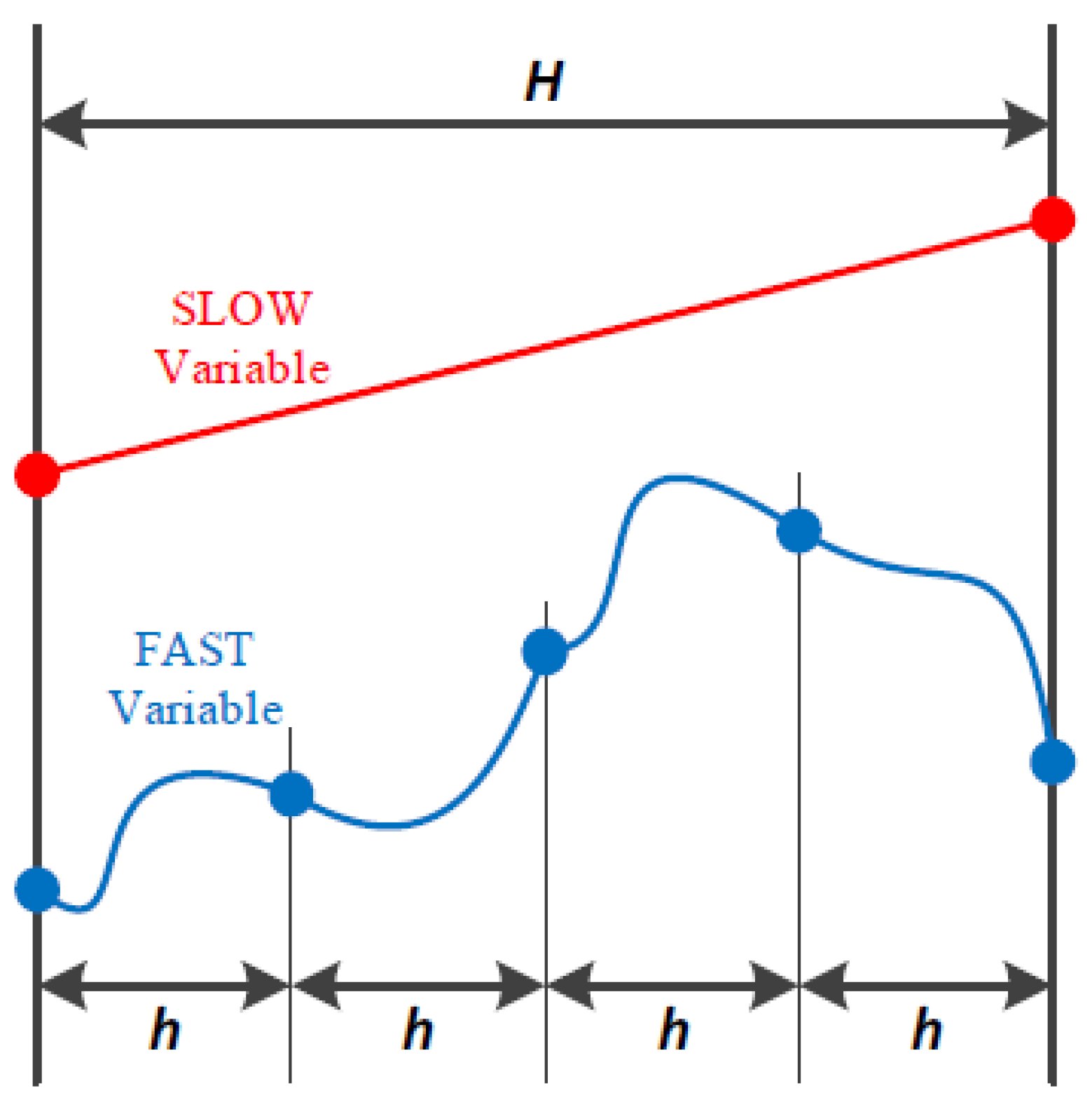
The multi-rate method provides an efficient integration technique for systems exhibiting a wide variety of time responses. The multi-rate method integrates different variables with different time steps [9]. It uses small time steps, called subintervals, for fast varying variables and larger time steps for more slowly varying ones. The subinterval integration approach, coupled with a longer main time step, allows for the network algebraic equations and slow dynamic equations to be evaluated much less frequently and thus computational benefits can be achieved, in particular for a large power system with very few fast variables. The method was applied to power system transient stability problem for the first time in [10] and advanced in [11,12]. Some widely used transient stability packages employ the multi-rate method [6,7,8].

As modern systems have become increasingly complex such as with the introduction of load dynamics, other power electronic models, and renewable energy sources, the system has become potentially more susceptible to numerical instability issues. Appropriate time steps should be carefully determined to prevent the numerical instability. However, commercial transient stability packages that utilize the multi-rate method often do not provide guidelines or a built-in function to select an appropriate subinterval time step. Instead, they use either a fixed value for all models of a type, or in the case of PowerWorld Simulator, heuristics based on model parameters. The tradeoff is between excessive computation if the interval is too short, and potential numeric instability if it is too long.

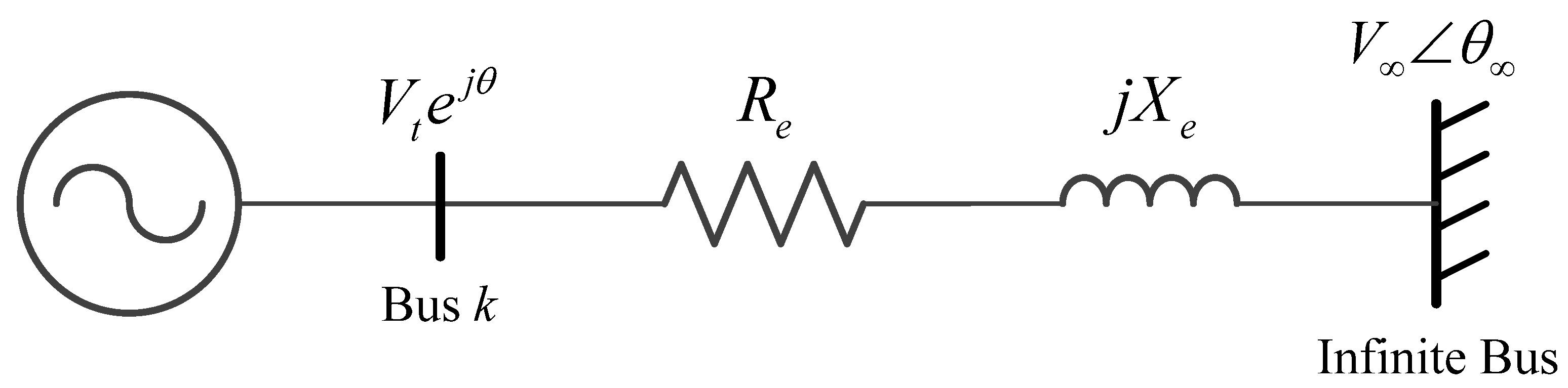
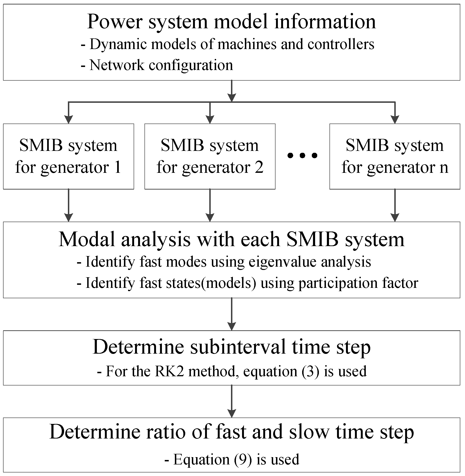
In this paper, a new subinterval selection approach is presented to determine the optimal numerical integration time step for the use with the multi-rate method. An appropriate subinterval can be determined by identifying how fast dynamic states are varying in the considered power system. The proposed approach uses modal analysis for single machine infinite bus (SMIB) models [3]. It analyzes the SMIB model eigenvalues, and thus fast dynamic states can be recognized. A primary source of fast dynamics in power systems are generators and their controllers. Instead of considering the whole system, the SMIB approach focuses on each generator with its controllers to identify the fast dynamics. Thus, the required computation for modal analysis with the SMIB approach can be quite modest, even for large systems. Depending on the SMIB approach eigenvalues, appropriate subinterval values can be determined to avoid numerical instability issues and to minimize the required computations.

This paper is organized as follows: Section 2 presents background information including the explicit numerical integration method, the multi-rate method and eigenvalue analysis with a SMIB system. In Section 3, a problem is defined and a new optimal time step selection method is then proposed. Section 4 illustrates simulation results with the GSO 37-bus case. The conclusion is made in Section 5.

2. Preliminary

2.1. Explicit Numerical Integration Method

Many commercial power system transient stability packages use explicit numerical integration methods, which estimate values for the next time step explicitly using present values. The second-order Runge-Kutta (RK2) method is one example of the explicit methods [2]. With an Ordinary Differential Equation (ODE), the RK2 method approximates the next time step value as:

$$x_n=x_{n-1}+h\cdot (\frac{1}{2}{k}_1+\frac{1}{2}{k}_2)$$

(1)

where, $k_1=f(x_{n-1},t_{n-1})$, $k_2=f(x_{n-1}+k_1,t_{n-1}+h)$, h: numerical integration time step.

When the simplest test equation $\dot{x}$ = λx is given, the region of stability is defined with Equation (2) and the region is shown in Figure 1. More detailed information about Equation (2) can be found in [12]:

$$\left|1+h\mathrm{\lambda }+\frac{1}{2}{(h\mathrm{\lambda })}^2\right|<1$$

(2)

As shown in Figure 1, for a real valued λ, stable region can be defined with Equation (3):

$$-2<h\mathrm{\lambda }<0$$

(3)

Based on Equation (3), minimum eigenvalues that the RK2 method can cover without numerical instability can be determined depending on the time step as shown in Table 1.

Figure 1. Region of stability of the second-order Runge-Kutta (RK2) method.

Figure 1. Region of stability of the second-order Runge-Kutta (RK2) method.

Table 1. Range of eigenvalues depending on the time step using the RK2 method.

Time Step (Cycle)	Range of Eigenvalue
1	−120 < λ < 0
0.25	−480 < λ < 0
0.1	−1200 < λ < 0
0.05	−2400 < λ < 0

Table 1. Range of eigenvalues depending on the time step using the RK2 method.

Time Step (Cycle)	Range of Eigenvalue
1	−120 < λ < 0
0.25	−480 < λ < 0
0.1	−1200 < λ < 0
0.05	−2400 < λ < 0

2.2. Multi-Rate Method

In practical power systems, only a small portion of the dynamic states are associated with fast dynamics and thus the use of very small time step for the entire simulation is not efficient in terms of computational time and storage. To avoid this computational burden, the multi-rate method that uses different time steps in a numerical integration scheme, has been commonly used [9]. The approach is shown in Figure 2. For the fast changing variables, a small time step (h) is used, while for the relatively slower changing variables, an integer multiple of the small time step (H) is used. As one can see from Figure 2, the ratio of the fast time step to the slow time step for this case is four. The equations for the fast variables must be solved at points where the slow ones have not been solved. This can be done by using a linear solution value interpolated from the slow variables [12].

Figure 2. Multi-rate method.

Figure 2. Multi-rate method.

2.3. SMIB System and Eigenvalue Analysis

The SMIB system models the machine of interest in detail, while the rest of the system is represented with a Thevenin equivalent circuit of a voltage behind an impedance. The Thevenin equivalent impedance at bus k is equal to the kth diagonal element of the Z matrix representing the entire power system [13,14]. The infinite bus voltage is set such that the total machine complex power output is the same in between the SMIB model and the entire system. In the SMIB system depicted in Figure 3, the multi-machine power system is reduced to a single machine that is connected to an infinite bus system in order to simplify the analysis and focus on one machine. The SMIB system does not capture the inter-area modes attributed to interaction among generators, but the local modes related to the generator including controllers can be identified.

Figure 3. Single machine infinite bus (SMIB) system.

Figure 3. Single machine infinite bus (SMIB) system.

For small perturbations, it is sufficient to analyze the linearized power system model. Linear models are simpler to understand and have many useful tools for analysis. One such tool is eigenvalue analysis. Eigenvalues indicate the system stability and how close the system is to becoming unstable. It also shows what frequencies and modes exist in the system, as well as how the system states interact with these modes.

The SMIB system can be modeled with Equations (4) and (5) which represent the power system dynamics and the stator and network algebraic equations, respectively [3]. The x variables show the dynamic state variables such as generator rotor angle and speed. The y variables show the algebraic variables such as the network bus voltage and angle:

$${\dot{x}}_{SMIB}=f(x_{SMIB},y_{SMIB})$$

(4)

$$0=g(x_{SMIB},y_{SMIB})$$

(5)

where:

• f: a vector of dynamic equations;
• g: a vector of algebraic equations;
• x_SMB: a vector of dynamic state variables of SMIB system;
• y_SMIB: a vector of algebraic state variables of SMIB system.

The power system equations shown in Equations (4) and (5) are nonlinear. Hence, they need to be linearized around the operating point in order to find out the eigenvalues. The equations of the linearized power system are given by Equations (6) and (7):

$$\text{Δ}{\dot{x}}_{SMIB}=A\text{Δ}{x}_{SMIB}+B\text{Δ}{y}_{SMIB}$$

(6)

$$0=C\text{Δ}{x}_{SMIB}+D\text{Δ}{y}_{SMIB}$$

(7)

where:

• $A={\frac{\partial f}{\partial x_{SMIB}}|}_{(x_{SMIB}^o,y_{SMIB}^o)}; B={\frac{\partial f}{\partial y_{SMIB}}|}_{(x_{SMIB}^o,y_{SMIB}^o)}; C={\frac{\partial g}{\partial x_{SMIB}}|}_{(x_{SMIB}^o,y_{SMIB}^o)}; D={\frac{\partial g}{\partial y_{SMIB}}|}_{(x_{SMIB}^o,y_{SMIB}^o)}; x_{SMIB}^o,y_{SMIB}^o$: SMIB system operating points.

Then, the system modal matrix is obtained by incorporating Equation (7) into (6) as following:

$$\text{Δ}\dot{x}=A_{sys}\text{Δ}x=(A-B{D}^{-1}C)\text{Δ}x$$

(8)

With the system modal matrix (A_sys), eigenvalues corresponding to fast local modes can be identified. Real components of eigenvalues provide information about how fast the corresponding modes are varying. The required time step to prevent the numerical instability can then be determined.

3. Problem Definition and Proposed Approach

3.1. Problem Definition

As described in Section 2.2, the multi-rate method requires the ratio of the fastest variables to the main time step (H in Figure 2) in order to determine the subinterval step size. However, it is not easy to identify the ratio with higher order, nonlinear power system models. Commercial transient stability packages usually use either a fixed value based on the model type, or heuristics that depend on model parameters. In designing such heuristics, in case of numerical instability for particular parameters, the subinterval time step is changed to a smaller value. On the other hand, choosing too small an interval can cause increased computation. Therefore, an optimal subinterval time step for use with the multi-rate method could remove unnecessary computations while avoiding numerical instability. Such an approach is presented in the next section.

3.2. Proposed Approach

In the approach presented here, the optimal subinterval time step is determined by analyzing the fast dynamics in each SMIB system. This works because the fast varying states are related to the local oscillations rather than inter-area oscillations. In the proposed method, the modal matrix is constructed by linearizing the SMIB system equations around an operating point. The SMIB eigenvalues can then be found, of which their magnitudes describe how rapidly the dynamics vary. By the use of the participation factor in linear system theory [2,3], it can be determined which dynamic states are associated with the fast modes. However, we note that in commercial packages, the subinterval is usually applied to all the differential equations for a particular model, such as an exciter. Hence, the participation factors only need to determine the particular model (e.g., the machine model, the exciter model, etc.) not the individual differential equations.

Finally, the subinterval step size for the fast dynamic states is determined by considering the region of stability equation of numerical integration method in use. For the RK2 method, explained in Section 2.1, Equation (3) is used to determine the appropriate step size. For the multi-rate method, the slow time step is obtained from the user specified value and the ratio between fast and slow time steps are then identified with Equation (9):

$$\text{Minimum subinterval ratio}=\frac{\text{Step size for slow variables (User specified)}}{\text{Required step size for fast variables}}$$

(9)

Figure 4 shows the overall procedure of the proposed approach. Note that the SMIB systems can be determined and analyzed quite quickly, so this approach could be efficiently used for a large system.

Figure 4. Flowchart of the proposed approach.

Figure 4. Flowchart of the proposed approach.

4. Case Study

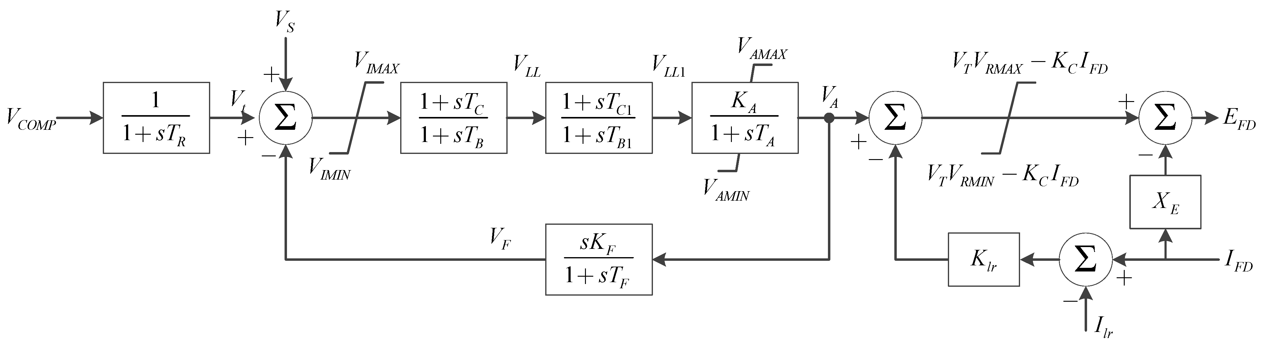
The proposed approach was tested with the PowerWorld Simulator, which provides SMIB eigenvalue analysis and uses a multi-rate numerical integration method [5]. The GSO 37-bus system shown in Figure 5 is used to demonstrate the proposed method. The case has nine generators, 25 loads and 57 branches [15]. One common exciter, the EXST1 (IEEE Type ST1 excitation system model) shown in Figure 6, quite commonly introduces very fast modes to the system because fast electronic controllers are incorporated. For test purposes, parameters for each of the EXST1 exciters for the two generators at bus 28 were changed as shown in Table 2.

Figure 5. GSO 37-bus system.

Figure 5. GSO 37-bus system.

Figure 6. Block diagram of EXST1 exciter.

Figure 6. Block diagram of EXST1 exciter.

Table 2. EXST1 Exciter model parameters.

Tr = 0	Vimax = 10	Vimin = −10	Tc = 1
Tb = 1	Ka = 150	Ta = 0.01	Vrmax = 3.6
Vrmin = 0	Kc = 0	Kf = 0.04	Tf = 0.4
Tc1 = 1	Tb1 = 1	Vamax = 99	Vamin = −99
Xe = 0	Ilr = 0	Klr = 0

Table 2. EXST1 Exciter model parameters.

Tr = 0	Vimax = 10	Vimin = −10	Tc = 1
Tb = 1	Ka = 150	Ta = 0.01	Vrmax = 3.6
Vrmin = 0	Kc = 0	Kf = 0.04	Tf = 0.4
Tc1 = 1	Tb1 = 1	Vamax = 99	Vamin = −99
Xe = 0	Ilr = 0	Klr = 0

4.1. SMIB Eigenvalue Analysis

With the test case considered, SMIB systems for all generators were created and modal analysis of each SMIB system was then performed. The results in Table 3 indicate that two big negative eigenvalues (−1602) are originated from the two generators at bus 28. The participation factors in Table 4 identify that these modes are solely contributed by exciter dynamic state V_A. Therefore, the required time step for the state V_A to avoid numerical instability can be determined with the real part of eigenvalue information, which represents how much the dynamic state varies.

Table 3. Single machine infinite bus (SMIB) eigenvalue analysis with the GSO 37-bus case.

Bus Number	Generator ID	Max Eigenvalues	Bus Number	Generator ID	Max Eigenvalues
28	1	−1602	54	1	−44
28	2	−1602	53	1	−42
31	1	−49	44	1	−42
14	1	−45	50	1	−38
48	1	−44	–	–	–

Table 3. Single machine infinite bus (SMIB) eigenvalue analysis with the GSO 37-bus case.

Bus Number	Generator ID	Max Eigenvalues	Bus Number	Generator ID	Max Eigenvalues
28	1	−1602	54	1	−44
28	2	−1602	53	1	−42
31	1	−49	44	1	−42
14	1	−45	50	1	−38
48	1	−44	–	–	–

Table 4. Participation factor of a generator at bus 28.

Real Part of Eigenvalues	Machine Angle	Machine Speed	Machine Eqp	Machine PsiDp	Machine PsiQpp	Exciter VA	Exciter VF
−1602	0	0	0.0001	0	0	1	0.0015
−45	0.0178	0.0183	0	0	0.9997	0	0
−32	0.0008	0.0007	0.0511	0.9987	0.0001	0.0001	0.0002
−22	0	0.0017	0	0	0.0002	0	0
−0.6	0.709	0.6983	0.0329	0.0056	0.0915	0	0.0007

Table 4. Participation factor of a generator at bus 28.

Real Part of Eigenvalues	Machine Angle	Machine Speed	Machine Eqp	Machine PsiDp	Machine PsiQpp	Exciter VA	Exciter VF
−1602	0	0	0.0001	0	0	1	0.0015
−45	0.0178	0.0183	0	0	0.9997	0	0
−32	0.0008	0.0007	0.0511	0.9987	0.0001	0.0001	0.0002
−22	0	0.0017	0	0	0.0002	0	0
−0.6	0.709	0.6983	0.0329	0.0056	0.0915	0	0.0007

4.2. Subinterval Step Size

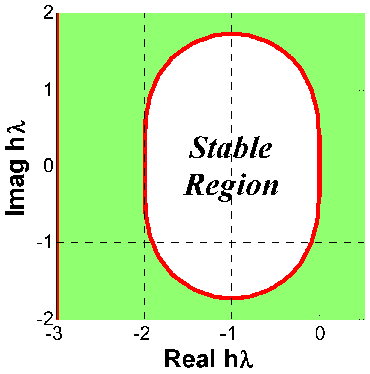
Due to the extremely fast modes (−1602), if a single rate approach was used, the time step for the entire system would need to be just 0.05 cycles to avoid numerical instability; this can be determined with Equation (3) and Table 1. On the other hand, the use of the multi-rate method can increase the step size by using the subinterval time step only for the dynamic states associated with the fastest modes (or as previously mentioned more commonly for all the states associated with the fast exciter model). When a quarter-cycle is selected as the step size for the entire simulation, the subinterval ratio should be greater than five based on Equation (9). The following equation shows how the ratio can be determined:

$$\begin{array}{l}\text{Minimum subinterval ratio}\\ =\frac{\text{Step size for slow variables (User speficied)}}{\text{Required step size for fast variables}}\\ =\frac{0.25\text{ cycles}}{0.05\text{ cycles}}=5\end{array}$$

4.3. Simulation Comparisons

PowerWorld Simulator has options that allow the user to override the built-in heuristics and directly specify the desired number of subintervals (in powers of two from two up to 128) for specific models. Hence, eight subintervals were chosen here to meet the minimum. In order to validate the performance of the proposed method, simulation comparisons were made by changing the subinterval step ratio. A three-phase bus to ground fault was applied at bus 28, which has the two EXST1 exciter generators. The fault was applied at 1.0 s and cleared at 1.1 s.

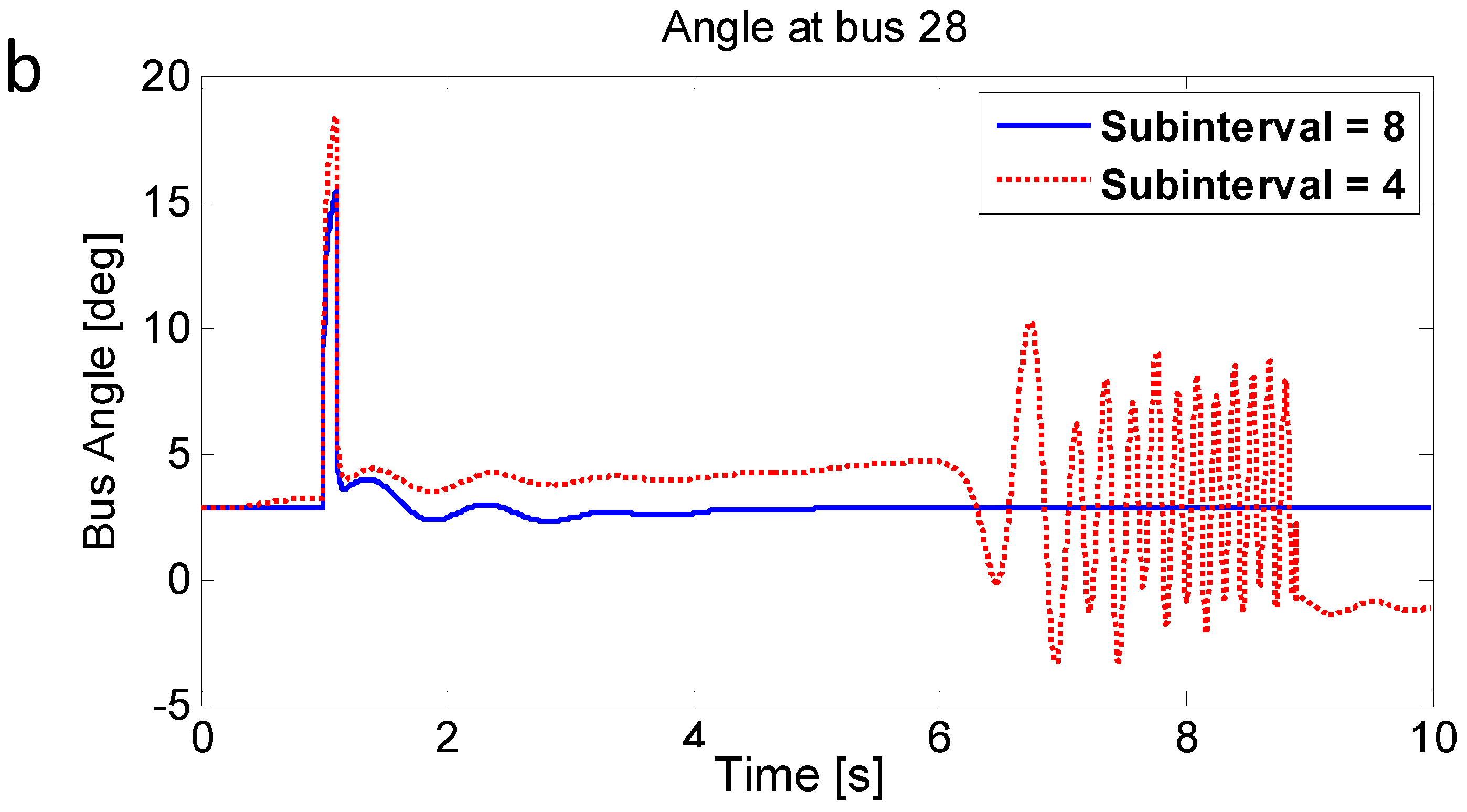
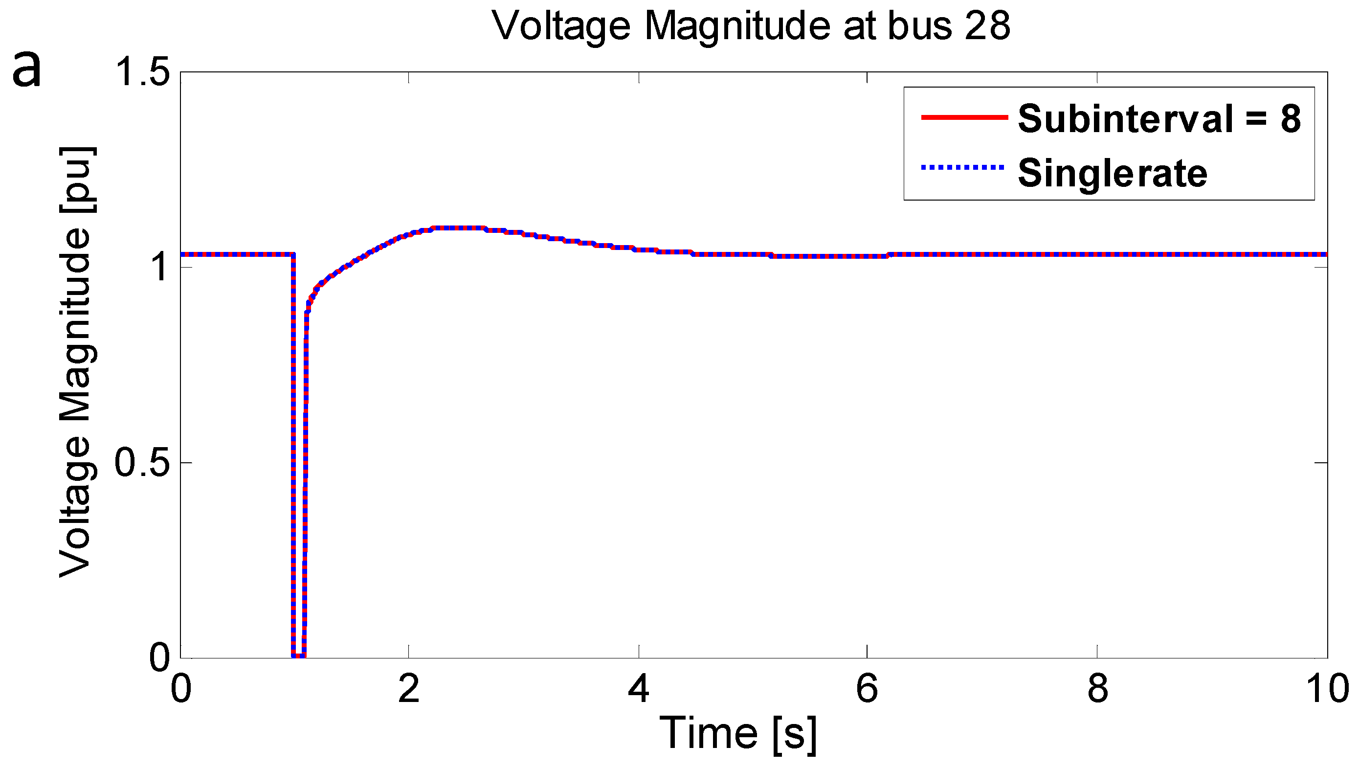
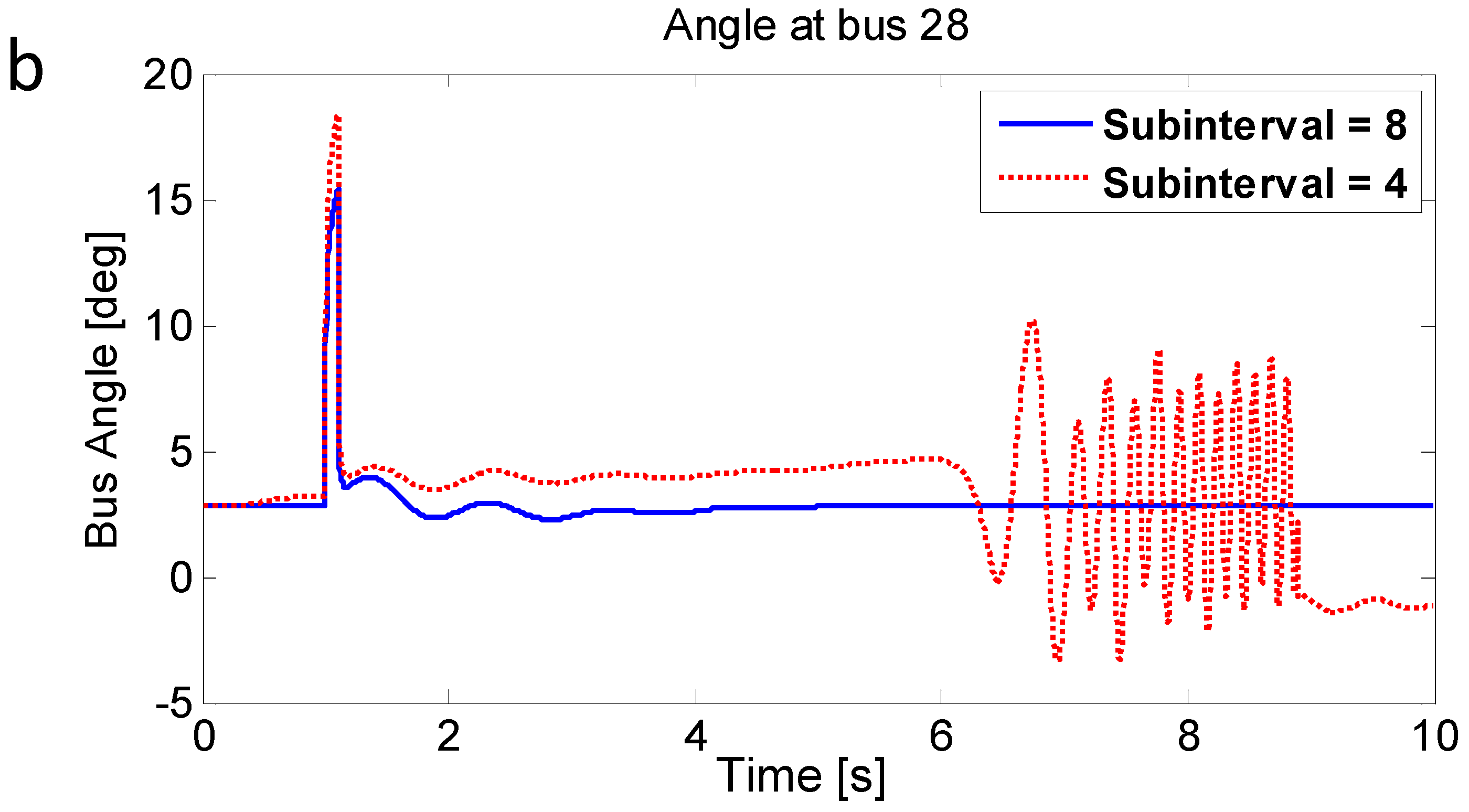
Figure 7 shows the bus voltage magnitude at bus 28 with two different subintervals (eight and four). When the subinterval was set to four, the simulation results show numerical instability even before the fault. This is because the subinterval step size for the fast variables is still bigger than the requirements. However, when the number of subinterval is increased to eight, it shows a stable simulation response. The appropriate step size for the fast ones is correctly estimated with the proposed method.

Figure 7. Simulation comparison between four and eight subintervals: (a) Voltage magnitude; (b) Angle.

Figure 7. Simulation comparison between four and eight subintervals: (a) Voltage magnitude; (b) Angle.

Next, a comparison was made between single rate and multi-rate methods. With the single rate method, 0.05 cycles was used for the time step, which is determined based on Table 1 to prevent numerical instability. For the multi-rate method, a quarter-cycle (0.25 cycles) for the slow dynamics and an eight subinterval option was used, which showed a stable response in Figure 7. As shown in Figure 8, the two simulation results are essentially identical. Table 5 shows the computation time with two different simulation approaches. The computation time is an average of running the simulation ten times and it does not include the required computation for SMIB eigenvalue analysis. Because the SMIBs are only associated with the local machines, they can be computed quite quickly. For example, in benchmarking, the PowerWorld simulator can perform complete SMIB eigenvalue analysis for a 3500 generator system within two seconds; for this nine generator system, the time would be less than a millisecond. The multi-rate method shows excellent computational performance by reducing the simulation time by about 80% compared to the single rate method.

Figure 8. Simulation comparison with single-rate and multi-rate methods: (a) Voltage magnitude; (b) Angle.

Figure 8. Simulation comparison with single-rate and multi-rate methods: (a) Voltage magnitude; (b) Angle.

Table 5. Computational time comparison.

Method Used	Time Step (Cycle)	Subinterval for Fast States	Computation Time (s)	Ratio of the Computation Time
Singlerate	0.05	–	51.3	1
Multirate	0.25	8	10.6	0.21

Table 5. Computational time comparison.

Method Used	Time Step (Cycle)	Subinterval for Fast States	Computation Time (s)	Ratio of the Computation Time
Singlerate	0.05	–	51.3	1
Multirate	0.25	8	10.6	0.21

5. Conclusions

When extremely large negative eigenvalues exist with power system dynamics being integrated using explicit methods, special considerations should be required to avoid numerical instability during power system transient stability analysis. The multi-rate numerical integration method is a common approach to reduce this computational issue. For the use of the multi-rate approach, the ratio between the user-specified time step and the subinterval for fast variables should be determined. This task is not easily identified in commercial transient stability packages. In this paper, an optimal subinterval selection method has been proposed. The method utilizes SMIB eigenvalue analysis, which identifies fast modes and dynamic states related to those modes. Based on the region of stability of numerical integration method in use, the appropriate step size can then be determined by comparing a user-defined time step for slow variables with very small time steps for fast variables. Optimum step size can reduce computational demands as well as avoid numerical instability. Test simulations with the GSO 37-bus case confirm that the proposed method provides quite a good performance in terms of accuracy and computational speed.

References

1. Fouad, A.A.; Aboytes, F.; Carvalho, V.F.; Corey, S.L.; Dhir, K.J.; Vierra, R. Dynamic security assessment practices in North America. IEEE Trans. Power Syst. 1998, 3, 1310–1321. [Google Scholar] [CrossRef]
2. Kundur, P. Power System Stability and Control; McGraw-Hill: New York, NY, USA, 1994. [Google Scholar]
3. Sauer, P.W.; Pai, M.A. Power System Dynamics and Stability; Prentice Hall: Upper Saddle River, NJ, USA, 1998. [Google Scholar]
4. Griffths, D.F.; Higham, D.J. Numerical Methods for Ordinary Differential Equations: Initial Value Problems; Springer: London, UK, 2010. [Google Scholar]
5. Stott, B. Power system dynamic response calculation. Proc. IEEE 1979, 67, 219–241. [Google Scholar] [CrossRef]
6. PowerWorld Corporation. Available online: http://www.powerworld.com/ (accessed on 1 September 2015).
7. Simens PSS/E. Available online: http://www.siemens.com/ (accessed on 1 September 2015).
8. General Electric Company. PSLF Version 18.0 User Manual; General Electric Company: Schenectady, NY, USA, 2011. [Google Scholar]
9. Gear, C. Multirate Methods for Ordinary Differential Equations; Technical Report; University of Illinois at Urbana-Champaign: Champaign, IL, USA, 1974. [Google Scholar]
10. Crow, M.L.; Chen, J.G. The multirate method for simulation of power system dynamics. IEEE Trans. Power Syst. 1994, 9, 1684–1690. [Google Scholar] [CrossRef]
11. Crow, M.L.; Chen, J.G. The multirate simulation of FACTS devices in power system dynamics. IEEE Trans. Power Syst. 1996, 11, 376–382. [Google Scholar] [CrossRef]
12. Chen, J.G.; Crow, M.L. A Variable Partitioning Strategy for the Multirate Method in Power Systems. IEEE Trans. Power Syst. 2008, 23, 259–266. [Google Scholar] [CrossRef]
13. Haque, M.H. A fast method for determining the voltage stability limit of a power system. Electr. Power Syst. Res. 1995, 32, 35–43. [Google Scholar] [CrossRef]
14. Haque, M.H. Novel method of assessing voltage stability of a power system using stability boundary in P–Q plane. Electr. Power Syst. Res. 2003, 64, 35–40. [Google Scholar] [CrossRef]
15. Glover, J.D.; Sarma, M.S.; Overbye, T.J. Power System Analysis and Design; Cengage Learning: Stamford, CT, USA, 2012. [Google Scholar]