A Neural Network Combined Inverse Controller for a Two-Rear-Wheel Independently Driven Electric Vehicle

Abstract

Vehicle active safety control is attracting ever increasing attention in the attempt to improve the stability and the maneuverability of electric vehicles. In this paper, a neural network combined inverse (NNCI) controller is proposed, incorporating the merits of left-inversion and right-inversion. As the left-inversion soft-sensor can estimate the sideslip angle, while the right-inversion is utilized to decouple control. Then, the proposed NNCI controller not only linearizes and decouples the original nonlinear system, but also directly obtains immeasurable state feedback in constructing the right-inversion. Hence, the proposed controller is very practical in engineering applications. The proposed system is co-simulated based on the vehicle simulation package CarSim in connection with Matlab/Simulink. The results verify the effectiveness of the proposed control strategy.

1. Introduction

Due to the drastic issues of environmental pollution and the energy-consumption crisis, many kinds of electric vehicles (EVs) are quickly being developed. Among them, the multi-wheel independently-driven EVs driven by either two or four motors are considered as a future trend. These motors are integrated into the drive wheels and can be controlled independently [1,2,3,4]. In this configuration, the motors directly drive the wheels so that the power train is shortened and EV efficiency is raised. Furthermore, since the driving/braking force of each wheel can be independently controlled, some vehicle safety system such as anti-brake system and direct yaw-moment control (DYC) become more flexible and feasible [5,6,7,8,9]. Moreover, the driving/braking force can be estimated in real time so that the observer or estimate technique can be applied easily. Therefore, the performances of the EVs are greatly improved.

It is well known that the vehicle dynamics are not completely independent in both directions. This is due to three major types of the coupling effects, namely the kinetic coupling, the tire force coupling and the weight shift coupling. These coupling effects become increasingly significant as maneuvers involve higher accelerations, larger tire forces, or reduced road friction [10]. It also has been verified that the dynamic coupling compensation does significantly improve the control performance of the vehicles [11]. However, the majority of the existing research has focused on either pure longitudinal or pure lateral control. In fact, the integration of both control problems is one of the most challenging issues. Only a handful of works have been reported on merging both control tasks into one goal [12,13,14]. Furthermore, as a typical nonlinear, time-varying and coupled system together with dynamic uncertainties, the vehicle precise dynamic model cannot be obtained in practices [15].

In fact, the performance of a vehicle active safety system depends not only on the control algorithm, but also on the accurate measurement of the vehicle motion states. In the DYC system, it is necessary to accurately measure yaw rate and sideslip angle. The yaw rate information is easily obtained by using low-cost gyro sensors, but unfortunately, the direct measurement of the sideslip angle is only provided by special devices (optical sensors or global positioning system inertial sensors combinations), which are nowadays very expensive and unsuitable for ordinary vehicles [16,17]. Thus, the sideslip angle must be estimated in real-time. For this reason, a variety of estimation methods have been studied extensively, such as Kalman filter/extended Kalman filter observers [18,19], recursive least square algorithms [20], adaptive observers [21] and else observers [22,23,24,25]. Most of these state observers and related algorithms rely heavily on an accurate tire model or a vehicle model. They are able to provide a satisfactory estimate results only these models are accurately known. However, the tire model and the vehicle model will vary during the vehicle operation.

Since the neural network (NN) has certain self-learning ability to adapt to environment and system characteristics, it has been used to estimate the sideslip angle [13,14,26,27]. In these literatures, the sideslip angle was considered as a map or function of the vehicle dynamics usually measured on board such as the lateral acceleration and the yaw rate. The results obtained seem to be promising, but these methods need a large amount of experimental data and the results depend on the data accuracy. Furthermore, these NN-based methods were seldom theoretically proved for its selection of training parameters. In addition, these methods have poor adaptability for the complex vehicle operating conditions. Therefore, these methods are limited in practice.

The main contribution of this paper is proposing a new control method, named NN combined inverse (NNCI) controller for the two-rear-motor independently driven EV to address two issues: (1) A new NN left inversion (NNLI) soft-sensor which combines the NN and the inverse system is employed to accurately estimate the sideslip angle; (2) The NN right-inversion (NNRI) controller is used to decouple the sideslip angle and the yaw rate. The remainder of this paper is organized as follows: Section 2 briefly describes the model of the vehicle, and Section 3 shows the design of the NNCI controller in detail. The simulated results are presented in Section 4. Finally, some conclusions and future works are presented in Section 5.

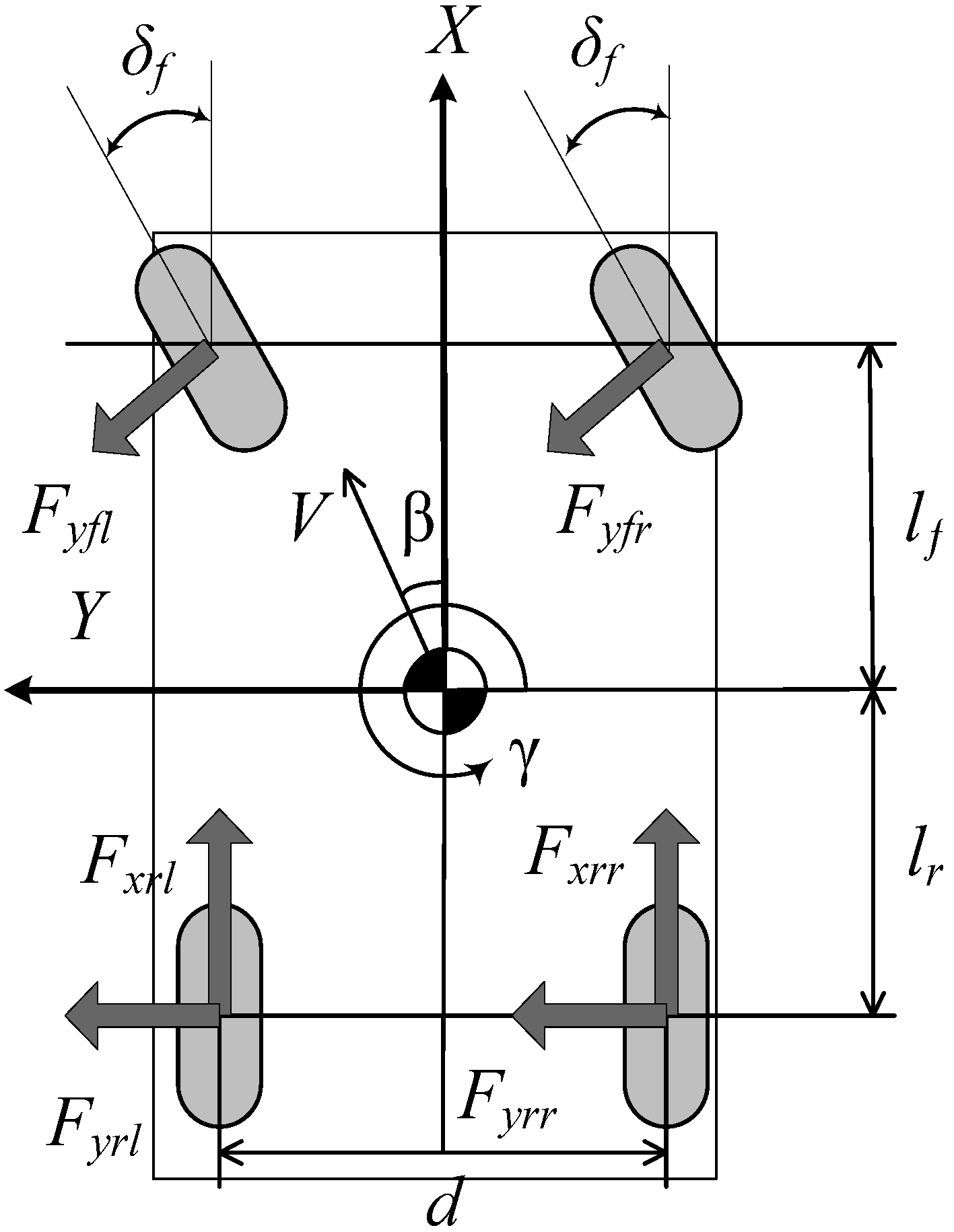
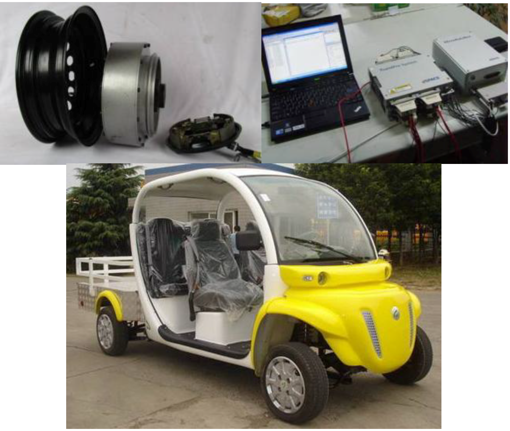
2. Two-Rear-Wheel Independently Driven EV

In this section, the vehicle with the front-wheel-steering and two-rear-wheel independently driven is assumed to be a constant velocity. By ignoring body roll, the vehicle model includes four degrees-of-freedom (4DOF), namely the lateral, the yaw motions and the two drive wheels. Figure 1 shows the two-wheel independently driven EV. The lateral and yaw motions of the vehicle can be expressed as follows:

(1)

where v_x is the longitudinal vehicle velocity; v_y is the lateral vehicle velocity; γ is the yaw rate and β is the sideslip angle; F_x and F_y are the longitudinal and lateral tire forces, respectively; The abbreviations fl, fr, rl and rr are front left, front right, rear left and rear right, respectively; δ_f is the front steering angle input; l_f and l_r are the distances from the center of gravity to front and rear axle; d is the width of the vehicle; m represents the vehicle mass; I_Z is the moment of inertia about the yaw axis.

Figure 1. Two-rear-wheel independently driven EV.

Figure 1. Two-rear-wheel independently driven EV.

The lateral tire forces of the front and rear tires are determined by using a linear approximation as follows:

F_yf = C_f α_f

(2)

F_yf = C_r α_r

(3)

where C_f and C_r are the lateral cornering stiffness of the front and rear tires; α_f and α_r are the slip angles of the front and rear tires. Furthermore, they can be expressed as:

(4)

(5)

The wheel rotational dynamics is represented by:

(6)

where ù_i is the tire rotational speed; R is the tire effective rolling radius; J_w is the wheel rotational inertia; T_i is the torque of the motor i ∈ {rr, rl}.

The additional yaw moment M_Z is:

(7)

By applying small angle assumption cosδ_f ≈ 1 and sinδ_f ≈ δ_f, the state equation of the 4DOF vehicle can be written as:

(8)

3. Neural Network Combined Inverse Control

The NN inverse method combines the merits of the inverse system theory and the NN technology together [28,29,30]. It solves the problems that the analytical inverse system method excessively depends on the exact system model and the expression of the inverse system.

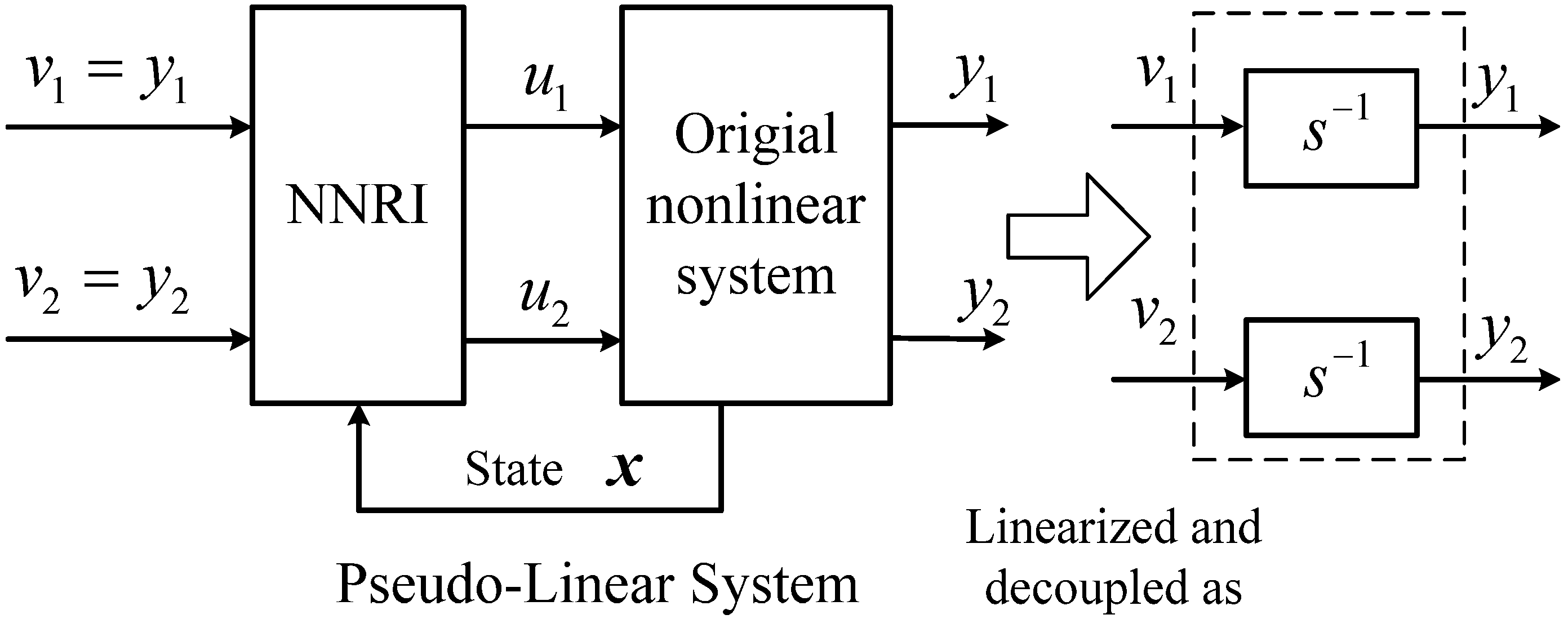
3.1. Neural Network Right Inversion Controller

For the system in Equation (8), the system state variable is:

x = (x₁,x₂)^T = (β,γ)^T

(9)

The system control variable is:

u = (u₁,u₂)^T = (δ_f,M_z)^T

(10)

and the system output variable is:

y = (y₁,y₂)^T = (β,γ)^T

(11)

The state equation of the 4DOF vehicle can be rewritten as:

ẋ = f (x,u)

(12)

where:

(13)

Using the Interactor algorithm [30], the Jacobi matrix is:

(14)

Due to:

(15)

the A(x,u) is nonsingular. Also, the system relative-order α = [α₁,α₂]^T = [1,1]^T, and the system order is α₁ + α₂ = 2. Therefore, this system is invertible. By setting and , the inverse system Φ can be described as:

u = Φ(x,v₁,v₂)

(16)

A back-propagation NN is trained offline to approximate the inverse system in Equation (16). When the learning process is over, the NNRI system is constructed. A pseudo-linear composite system can be obtained by cascading this NNRI system before the original nonlinear system. Then, a complex multi-variable vehicle dynamic system with strong coupling and uncertainties is linearized and decoupled into two linear integral subsystems (ã subsystem and â subsystem), as shown in Figure 2. As a result, the closed-loop control can be realized by using linear control theory.

Figure 2. Diagram of pseudo-linear system.

Figure 2. Diagram of pseudo-linear system.

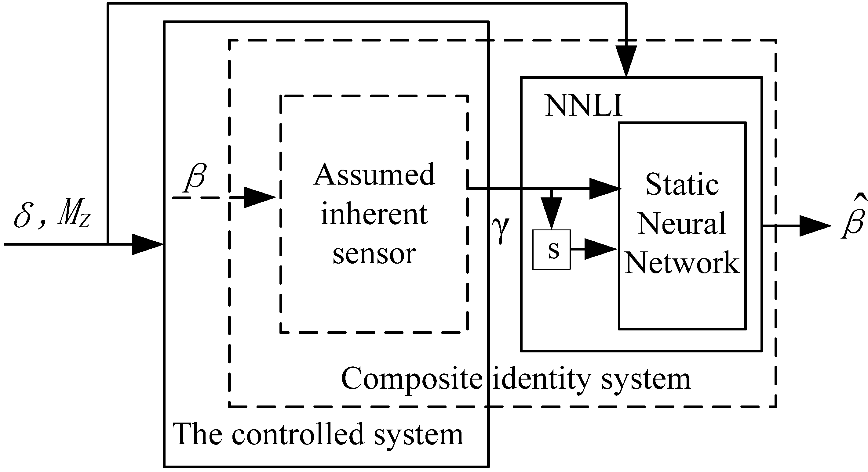
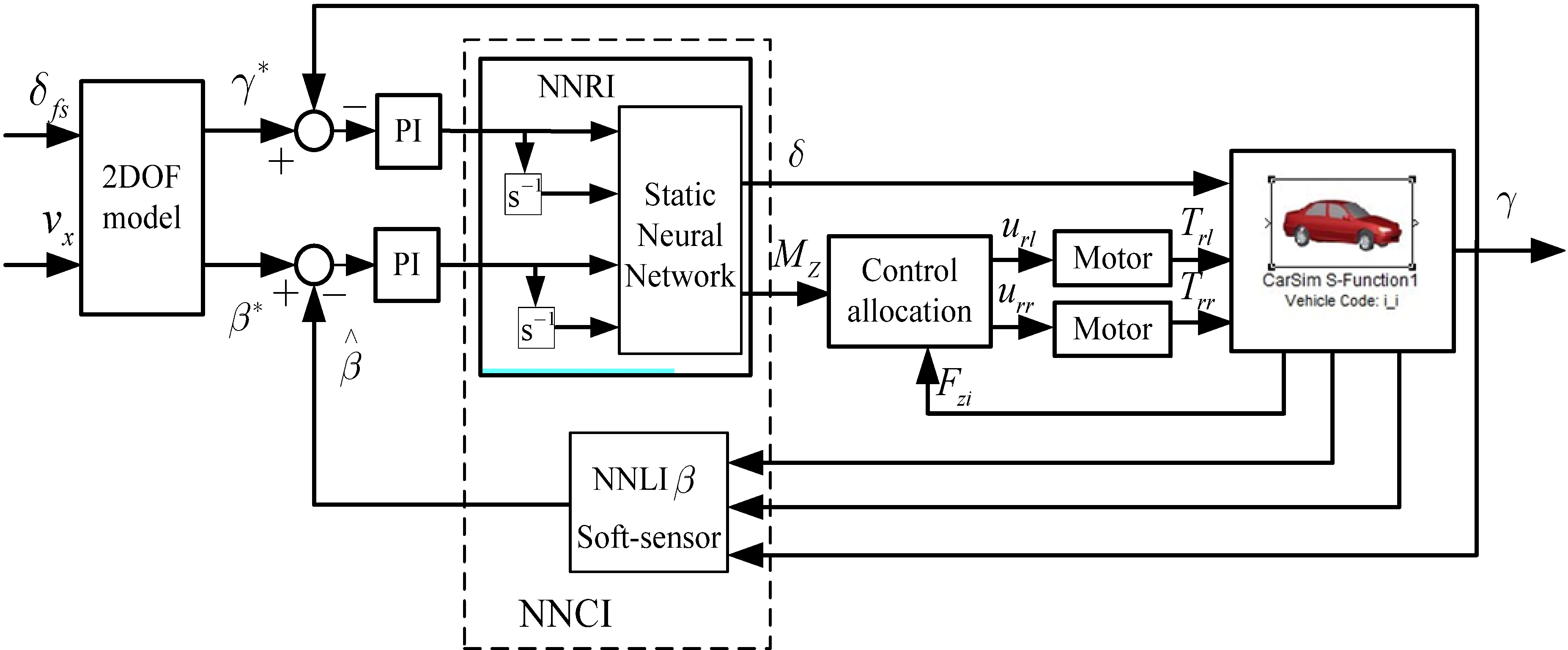
3.2. Neural Network Left Inversion Sideslip Angle Soft-Sensor

From Equation (16), it can be known that the input variables of the inverse system are the derivative of output variables of the original vehicle system i.e., and . In other words, to construct the NNRI controller, it is essential to obtain the state variables. As mentioned above, the soft-sensor to estimate the sideslip angle is needed for some reasons such as system cost.

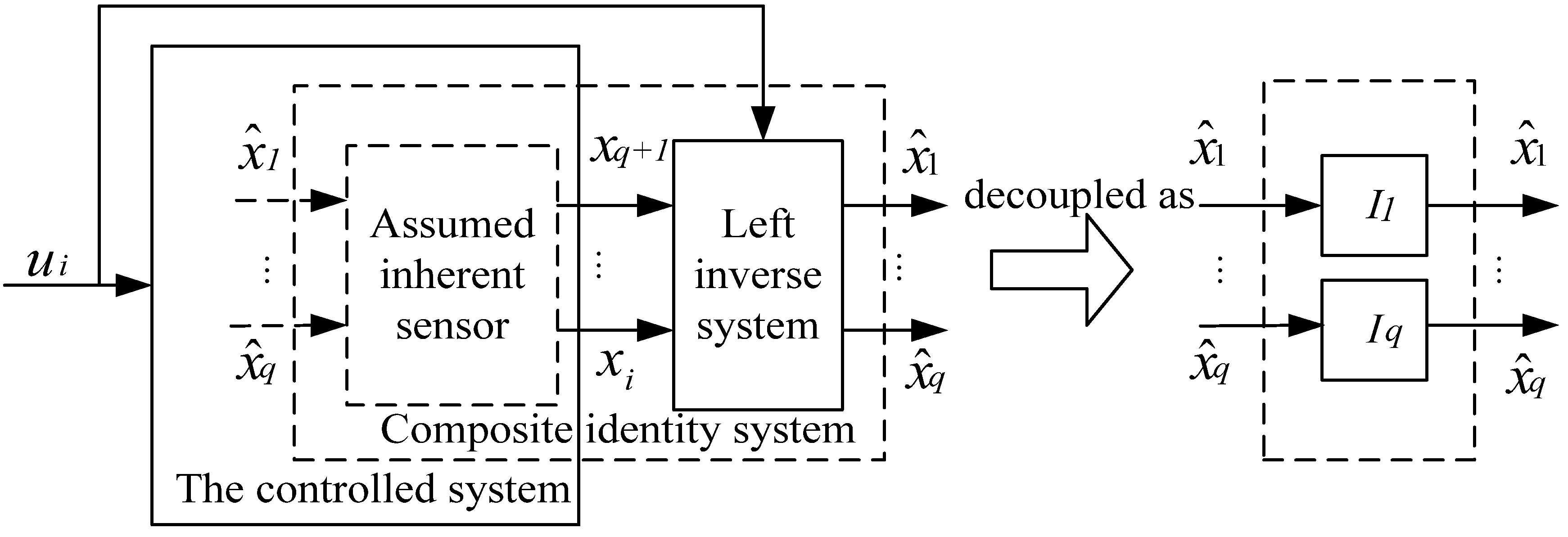
Generally speaking, for a non-linear system, in its interior, it can be assumed that there exists an “assumed inherent sensor” subsystem as shown in Figure 3. The variables (can be estimated) are the inputs of the subsystem, while the variables x_q+1⋯x_i which can be measured directly are the outputs. The variables u_i are the input variables of the controlled system. If a left inversion of the “assumed inherent sensor” can be constructed and cascaded behind the assumed inherent sensor, a so-called composite identity system is obtained, whose outputs would be the identity mapping of its inputs. It means that the outputs of the “assumed inherent sensor” inversion will reproduce completely the inputs of the “assumed inherent sensor”. Therefore, the non-directly measured variables of the controlled system can be estimated from the variables x_q+1⋯x_i, which can be measured directly.

Figure 3. Measuring principle based on left inversion.

Figure 3. Measuring principle based on left inversion.

For the system in Equation (12), its state variable is:

x = (x₁,x₂,x₃,x₄)^T = (γ,β,v_x,a_x)^T

(17)

The input of the system is:

u = (u₁,u₂)^T = (δ_f,M_z)^T

(18)

The directly measured variable is:

z = (z₁,z₂,z₃)^T = (γ,v_x,a_x)^T

(19)

The non-directly measured variable is:

x = (x₁)^T = (β)^T

(20)

According to the modeling algorithm, the Jacobian matrix rank is obtained:

(21)

Since the rank is not equal to the number of the non-directly measured variables, it can further derivate as:

(22)

Therefore, the model of the “assumed inherent sensor” is left invertible. And the left inversion of the “assumed inherent sensor” for sideslip angle can be written as:

(23)

Since the system is complex in mathematical model, it is difficult to construct the above “assumed inherent sensor” inversion by analytic means. Hence, another static NN is used to approximate the above nonlinear function in Equation (23). Then, the NNLI dynamic soft-sensor is finally completed, which is composed of a static NN and a series of differentiators. It simplifies the construction of the proposed NN-based soft-sensor in practical use, while is strict enough in theory. The structure of the NNLI sideslip angle soft-sensor is shown in Figure 4.

Figure 4. NNLI sideslip angle soft-sensor.

Figure 4. NNLI sideslip angle soft-sensor.

3.3. Neural Network Combined Inverse Controller

Taking full advantage of the powerful ability of the left-inversion soft-sensor to estimate system state, the combination of NNRI controller with NNLI soft-sensor results in a new nonlinear control method, which is called NNCI control. The NNLI soft-sensor can estimate the sideslip angle, while the NNRI is used to decouple the sideslip angle and the yaw rate. Then, the proposed NNCI controller not only linearizes and decouples the original nonlinear system, but also directly obtains immeasurable state feedback in constructing the right-inversion.

After being linearized by the proposed NNCI, the ultimate closed vehicle active safety system can be controlled by a traditional Proportional-Integral (PI) controller as shown in Figure 5, where the 2DOF model is used to generate the desired yaw rate and the desired sideslip angle [9]. The additional yaw moment M_Z is allocated into the torques of two driving motors through the control allocation. The control allocation method is that one side of the wheel driving torque decreases, while the other side of the wheel driving torque increases.

Figure 5. Block diagram of proposed NNCI control system.

Figure 5. Block diagram of proposed NNCI control system.

4. Verification

The performance of the control algorithm is evaluated by Matlab/Simulink-CarSim cosimulation. A vehicle with two motors at the rear wheels is developed using CarSim. The NNRI controller and NNLI soft-sensor are constructed by using Matlab/Simulink. To verify proposed controller, the dynamics of the NNCI vehicle are compared with those of the integrated AFS + DYC one.

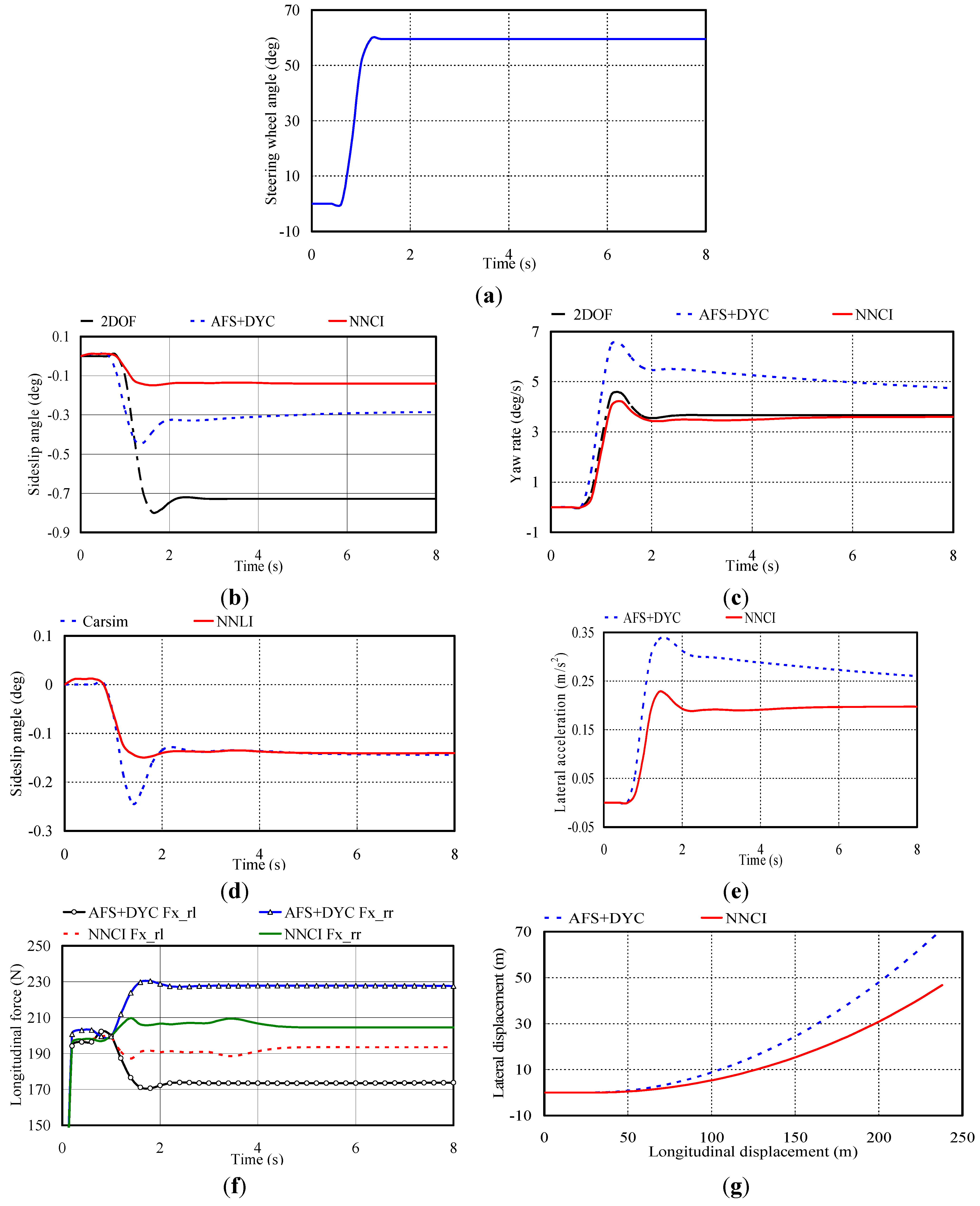
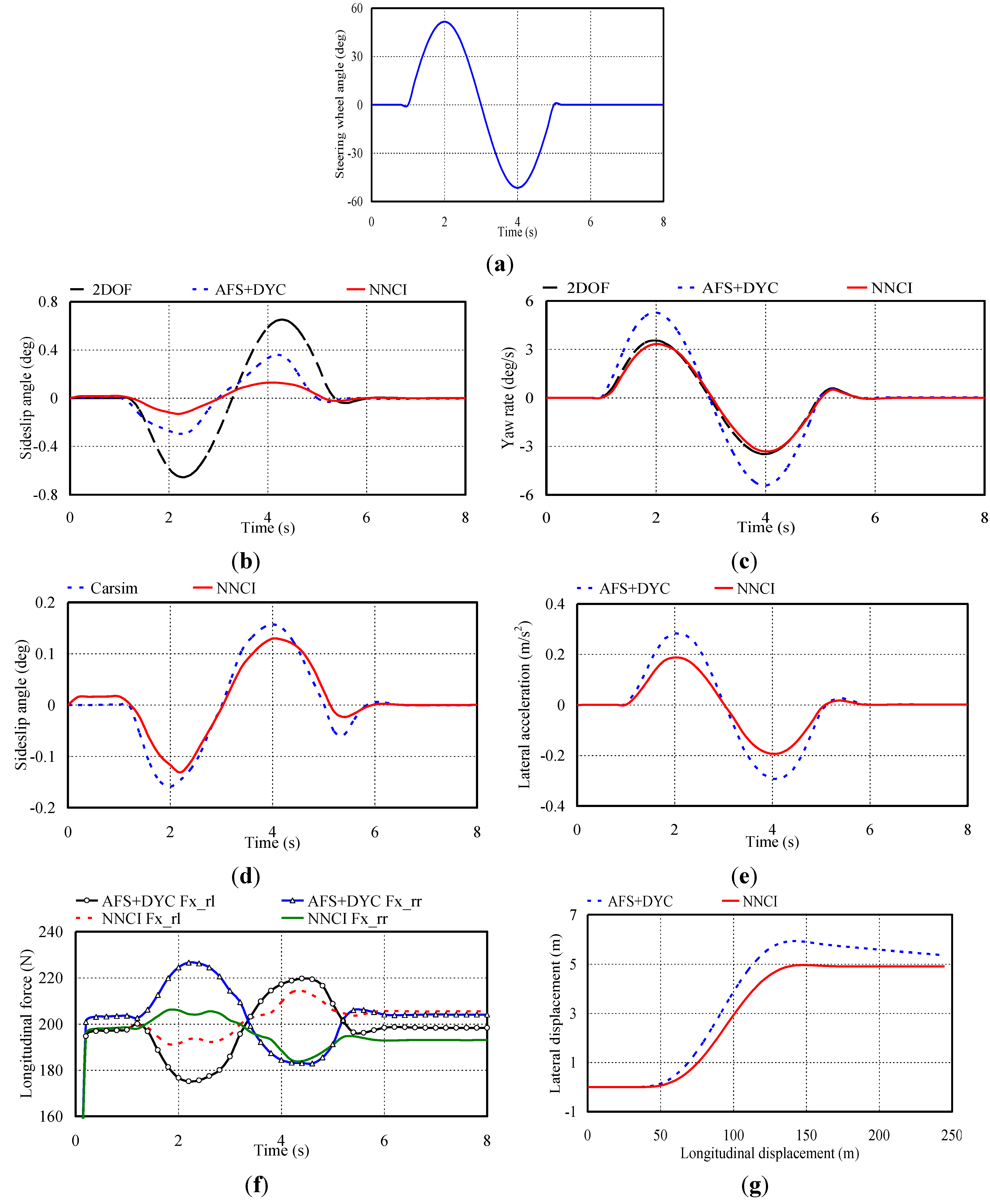
4.1. Ramp Steering Maneuver

Firstly, in the ramp steering maneuver, the proposed NNCI vehicle is evaluated as compared with the AFS + DYC one. A ramp steering maneuver is performed by comprising a ramp steering wheel input shown in Figure 6a. The vehicle travels on a wet road (μ = 0.4) at a constant speed of 100 km/h. In this case, the NNCI vehicle has smaller slip angle than the AFS + DYC one, as shown in Figure 6b. This is due to the employed NNCI controller, which decouple the yaw rate and the slip angle. While as shown in the Figure 6c,e, the NNCI vehicle has slower yaw rate and smaller lateral acceleration than the AFS + DYC one. As a result, the NNCI vehicle has an increased turning radius as shown in Figure 6g. This is because NNCI controller needs longer time to perform the control strategy than AFS + DYC one. Figure 6d shows the NNLI soft-sensor’s estimated results in the ramp steering maneuver. Furthermore, from the Figure 6f, the longitudinal forces of the two rear wheels of the NNCI vehicle are smaller than those of the AFS + DYC one.

Figure 6. Comparison of AFS + DYC vehicle and NNCI vehicle in ramp steering maneuver. (a) Ramp steering; (b) Sideslip angle; (c) Yaw rate; (d) Estimated sideslip angle; (e) Lateral acceleration; (f) Two-rear-wheel longitudinal forces; (g) Lateral displacement.

Figure 6. Comparison of AFS + DYC vehicle and NNCI vehicle in ramp steering maneuver. (a) Ramp steering; (b) Sideslip angle; (c) Yaw rate; (d) Estimated sideslip angle; (e) Lateral acceleration; (f) Two-rear-wheel longitudinal forces; (g) Lateral displacement.

4.2. Single Lane Change Steering Maneuver

Secondly, they are compared in the single lane change maneuver. A single lane change is performed comprising a single sine steering wheel input shown in Figure 7a. The vehicle also travels on a wet road (μ = 0.4) at a constant speed of 100 km/h. The yaw rate and the slip angle responses to the sine steering are presented in Figure 7b,c. The NNCI vehicle traces the desired yaw rate more precisely than the AFS + DYC one. In particular, the NNCI vehicle has much lower sideslip angle than the AFS + DYC one, and the yaw rate and sideslip angle are decoupled very well. The longitudinal forces of the two rear wheels are compared in Figure 7f. The lateral displacement of the NNCI vehicle is also smaller than that of the AFS + DYC one as shown in Figure 7g.

Figure 7. Comparison of AFS+DYC vehicle and NNCI vehicle in single lane change maneuver. (a) Single lane change steering; (b) Sideslip angle; (c) Yaw rate; (d) Estimated sideslip angle; (e) Lateral acceleration; (f) Two rear wheels longitudinal forces; (g) Lateral displacement.

Figure 7. Comparison of AFS+DYC vehicle and NNCI vehicle in single lane change maneuver. (a) Single lane change steering; (b) Sideslip angle; (c) Yaw rate; (d) Estimated sideslip angle; (e) Lateral acceleration; (f) Two rear wheels longitudinal forces; (g) Lateral displacement.

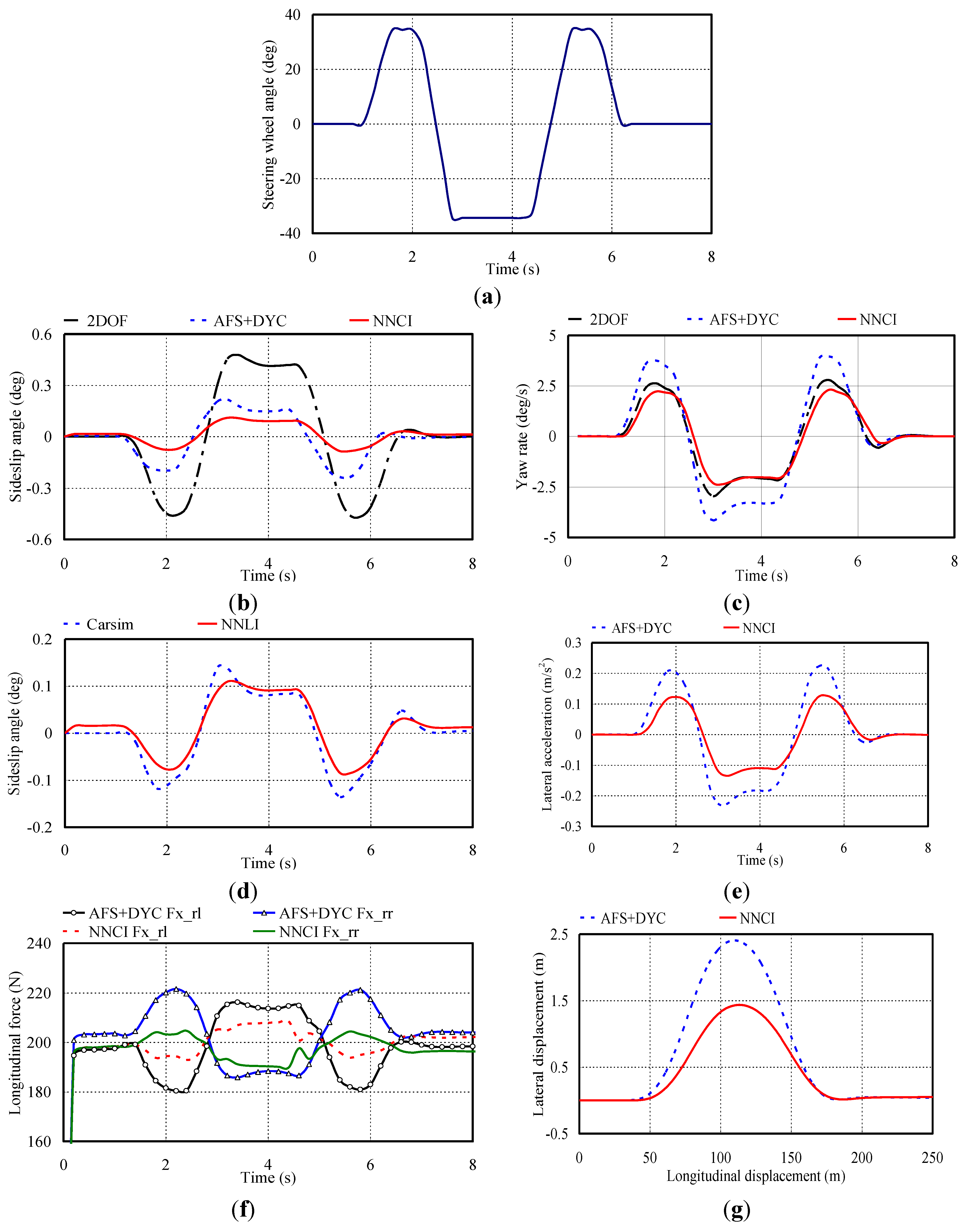
4.3. Double Lane Changing Maneuver

Finally, in the double lane changing maneuver shown in Figure 8a, the yaw rate and the slip angle responses are compared in Figure 8b,c. The NNLI estimated result is displayed in Figure 8d. The lateral acceleration of the NNCI vehicle is less than 0.2 g on the slippery road surfaces in Figure 8e. It is indicated that controlling the vehicle sideslip angle is beneficial to maintain the vehicle stable in this critical driving conditions. The longitudinal forces of the two rear wheels and the vehicle trajectories are also shown in Figure 8f,g. It can be concluded that the AFS + DYC vehicle provide larger lateral displacements than the NNCI one owing to the large yaw rate and lateral acceleration.

These three maneuver results verify that the actual and estimated values of the sideslip angle agree well. Therefore, the NNLI soft-sensor can accurately estimate the sideslip angle. On the other hand, both vehicles can successfully track the desired yaw rate as well as minimize the sideslip angle to maintain stable. Meanwhile, by comparing Figure 6 Figure 7 and Figure 8, it can be seen that the sideslip angle of the NNCI vehicle is smaller than that of the AFS + DYC one. Therefore, the stability of the NNCI vehicle is significantly improved in critical driving condition.

In contrast, the AFS + DYC vehicle has relatively higher yaw rate than the NNCI one, because the proposed decoupling controller needs longer time to calculate the additional yaw moment. Therefore, compared with the AFS + DYC vehicle, the NNCI one decreases the maneuverability, but it significantly decouples the yaw rate and sideslip angle. Furthermore, in all the cases, the longitudinal forces of the two rear wheels of the NNCI vehicle are smaller than those of the AFS + DYC one. This means that comparing with the integrated AFS + DYC controller, the NNCI one needs lower electric power energy to drive the EV under the same operation condition.

Figure 8. Comparison of AFS + DYC vehicle and NNCI vehicle in double lane changing maneuver. (a) Double lane changing steering; (b) Sideslip angle; (c) Yaw rate; (d) Estimated sideslip angle; (e) Lateral acceleration; (f) Two rear wheels longitudinal forces; (g) Lateral displacement.

Figure 8. Comparison of AFS + DYC vehicle and NNCI vehicle in double lane changing maneuver. (a) Double lane changing steering; (b) Sideslip angle; (c) Yaw rate; (d) Estimated sideslip angle; (e) Lateral acceleration; (f) Two rear wheels longitudinal forces; (g) Lateral displacement.

5. Conclusions and Future Works

In this paper, a new NNCI decoupling controller has been designed for the two-rear-wheel independently driven EV in order to improve the maneuverability and stability performance. To estimate the sideslip angle, an “assumed inherent sensor” left inversion has been treated as the dynamic soft-sensor, which consists of a NN and a series of differentiators. The yaw rate and the sideslip angle have been decoupled by using the proposed NNCI controller. Also, the NNLI soft-sensor can estimate the sideslip angle accurately. A co-simulation model has been developed and the results have been given, it has been proved that the proposed vehicle offers improved stability and maneuverability. In the future, these results will be experimentally verified based on a two-rear-wheel independently driven prototype EV which shown in Figure 9.

Figure 9. In-wheel motor, dSPACE and prototype EV.

Figure 9. In-wheel motor, dSPACE and prototype EV.

References

1. Hori, Y. Future vehicle driven by electricity and control-research on four-wheel-motored “UOT March II”. IEEE Trans. Ind. Electron. 2004, 51, 954–962. [Google Scholar] [CrossRef]
2. Wang, R.; Chen, Y.; Feng, D.; Huang, X.; Wang, J. Development and performance characterization of an electric ground vehicle with independently actuated in-wheel motors. J. Power Sources 2011, 196, 3962–3971. [Google Scholar] [CrossRef]
3. Chau, K.T.; Chan, C.C.; Liu, C. Overview of permanent magnet brushless drives for electric and hybrid electric vehicles. IEEE Trans. Ind. Electron. 2008, 55, 2246–2257. [Google Scholar] [CrossRef] [Green Version]
4. Magallan, G.A.; Angelo, C.H.D.; García, G.O. Maximization of the traction forces in a 2WD electric vehicle. IEEE Trans. Veh. Technol. 2011, 60, 369–380. [Google Scholar] [CrossRef]
5. Long, B.; Lim, S.T.; Ryu, J.H.; Chong, K.T. Energy-regenerative braking control of electric vehicles using three-phase brushless direct-current motors. Energies 2014, 7, 99–114. [Google Scholar]
6. Xu, G.; Li, W.; Xu, K.; Song, Z. An Intelligent regenerative braking strategy for electric vehicles. Energies 2011, 4, 1461–1477. [Google Scholar] [CrossRef]
7. Shuai, Z.; Zhang, H.; Wang, J.; Li, J.; Ouyang, M. Lateral motion control for four-wheel-independent-drive electric vehicles using optimal torque allocation and dynamic message priority scheduling. Control Eng. Pract. 2014, 24, 55–66. [Google Scholar] [CrossRef]
8. Kang, J.; Yoo, J.; Yi, K. Driving control algorithm for maneuverability, lateral stability, and rollover prevention of 4WD electric vehicles with independently driven front and rear wheels. IEEE Trans. Veh. Technol. 2011, 60, 2987–3001. [Google Scholar] [CrossRef]
9. Mirzaei, M. A new strategy for minimum usage of external yaw moment in vehicle dynamic control system. Transp. Res. Part C Emerg. Technol. 2010, 18, 213–224. [Google Scholar] [CrossRef]
10. Lim, E.H.M.; Hedrick, J.K. Lateral and longitudinal vehicle control coupling for automated vehicle operation. In Proceedings of the American Control Conference, San Diego, CA, USA, 2–4 June 1999; pp. 3676–3680.
11. Mrino, R.; Cinili, F. Input-output decoupling control by measurement feedback in four wheel steering vehicles. IEEE Trans. Control Syst. Technol. 2009, 17, 1163–1172. [Google Scholar] [CrossRef]
12. Jia, Y. Robust control with decoupling performance for steering and traction of 4WS vehicles under velocity-varying motion. IEEE Trans. Control Syst. Technol. 2000, 8, 554–569. [Google Scholar] [CrossRef]
13. Kumarawadu, S.; Lee, T. Neuroadaptive output tracking of fully autonomous road vehicles with an observer. IEEE Trans. Intell. Transp. Syst. 2009, 10, 335–345. [Google Scholar] [CrossRef]
14. Fernando, W.U.N.; Kumarawadu, S. Discrete-time neuroadaptive control using dynamic state feedback with application to vehicle motion control for intelligent vehicle highway systems. IET Control Theory Appl. 2010, 4, 1465–1477. [Google Scholar] [CrossRef]
15. Zhang, Z.; Chau, K.T.; Wang, Z. Analysis and stabilization of chaos in the electric-vehicle steering system. Trans. Veh. Technol. 2013, 62, 118–126. [Google Scholar] [CrossRef] [Green Version]
16. Bevly, D.M.; Ryu, J.; Gerdes, J.C. Integrating INS sensors with GPS measurements for continuous estimation of vehicle sideslip, roll, and tire cornering stiffness. IEEE Trans. Intell. Transp. Syst. 2006, 7, 483–493. [Google Scholar] [CrossRef]
17. Nam, K.; Oh, S.; Fujimoto, H. Estimation of sideslip and roll angles of electric vehicles using lateral tire force sensors through RLS and kalman filter approaches. IEEE Trans. Ind. Electron. 2013, 60, 988–1000. [Google Scholar] [CrossRef]
18. Wenzel, T.A.; Burnham, K.J.; Blundell, M.V.; Williams, R.A. Dual extended kalman filter for vehicle state and parameter estimation. Veh. Syst. Dyn. 2006, 44, 153–171. [Google Scholar] [CrossRef]
19. Doumiati, M.; Victorino, A.C.; Charara, A.; Lechner, D. On board real-time estimation of vehicle lateral tire-road forces and sideslip angle. IEEE ASME. Trans. Mechatron. 2011, 16, 601–614. [Google Scholar] [CrossRef]
20. Ding, N.; Taheri, S. Application of recursive least square algorithm on estimation of vehicle sideslip angle and road friction. Math. Probl. Eng. 2010. [Google Scholar] [CrossRef]
21. You, S.; Hahn, J.; Lee, H. New adaptive approaches to real-time estimation of vehicle sideslip angle. Control Eng. Pract. 2009, 17, 1367–1379. [Google Scholar] [CrossRef]
22. Gao, X.; Yu, Z.; Neubeck, J.; Wiedemann, J. Sideslip angle estimation based on input-output linearization with tire-road friction adaptation. Veh. Syst. Dyn. 2010, 48, 217–234. [Google Scholar] [CrossRef]
23. Solmaz, S. Simultaneous estimation of road friction and sideslip angle based on switched multiple non-linear observers. IET Control Theory Appl. 2012, 6, 2235–2247. [Google Scholar] [CrossRef]
24. Nam, K.; Fujimoto, H.; Hori, Y. Lateral stability control of in-wheel-motor-driven electric vehicles based on sideslip angle estimation using lateral tire force sensors. IEEE Trans. Veh. Technol. 2012, 61, 1972–1985. [Google Scholar] [CrossRef]
25. Piyabongkarn, D.; Rajamani, R.; Grogg, J.; Lew, J. Development and experimental evaluation of a slip angle estimator for vehicle stability control. IEEE Trans. Control Syst. Technol. 2009, 17, 78–88. [Google Scholar] [CrossRef]
26. Melzi, S.; Sabbioni, E. On the vehicle sideslip angle estimation through neural networks: Numerical and experimental results. Mech. Syst. Signal Process. 2011, 25, 2005–2019. [Google Scholar] [CrossRef]
27. Subudhi, B.; Ge, S.S. Sliding-mode-observer-based adaptive slip ratio control for electric and hybrid vehicles. IEEE Trans. Intell. Transp. Syst. 2012, 13, 1617–1626. [Google Scholar] [CrossRef]
28. Dai, X.; Wang, W.; Ding, Y. “Assumed inherent sensor” inversion based ANN dynamic soft-sensing method and its application in erythromycin fermentation process. Comput. Chem. Eng. 2006, 30, 1203–1225. [Google Scholar] [CrossRef]
29. Ding, Y.; Liu, G.; Dai, X. Soft-sensing method based on modified ANN inversion and its application in erythromycin fermentation. In Proceedings of the IEEE International conference on Information and Automation, Shenyang, China, 6–8 June 2012; pp. 900–905.
30. Liu, G.; Yu, K.; Zhao, W. Neural network based internal model decoupling control of three-motor drive system. Electr. Power Comp. Syst. 2012, 40, 1621–1638. [Google Scholar] [CrossRef]