SDP Policy Iteration-Based Energy Management Strategy Using Traffic Information for Commuter Hybrid Electric Vehicles

Abstract

This paper demonstrates an energy management method using traffic information for commuter hybrid electric vehicles. A control strategy based on stochastic dynamic programming (SDP) is developed, which minimizes on average the equivalent fuel consumption, while satisfying the battery charge-sustaining constraints and the overall vehicle power demand for drivability. First, according to the sample information of the traffic speed profiles, the regular route is divided into several segments and the statistic characteristics in the different segments are constructed from gathered data on the averaged vehicle speeds. And then, the energy management problem is formulated as a stochastic nonlinear and constrained optimal control problem and a modified policy iteration algorithm is utilized to generate a time-invariant state-dependent power split strategy. Finally, simulation results over some driving cycles are presented to demonstrate the effectiveness of the proposed energy management strategy.

1. Introduction

During the recent decade, HEVs have been a research focus in the trend to reduce fuel consumption and emissions. The improvement of fuel economy in HEVs strongly depends on the energy management strategy employed. The primary objective of any energy management strategy is to satisfy the driver’s power demand by determining the power distribution between the engine and the electric machines, as well as the optimal gear ratio of the transmission, if any, to minimize fuel consumption and simultaneously satisfying other constraints such as regulation of the battery state of charge (SOC), emissions and drivability. In order to meet these requirements, many optimal control strategies for HEVs have been proposed in the past. For instance, the dynamic programming (DP) approach dependent on the specific driving cycle was investigated in several publications [1,2,3,4,5]. Stochastic dynamic programming (SDP), which exploits a probabilistic distribution of the power demand obtained from many driving cycles, is suggested in [6,7,8,9]. Moreover, the equivalent consumption minimization strategy (ECMS) are suggested in [9,10,11], Pontryagin’s minimum principle (PMP) is introduced as an optimal control solution in [12,13,14], and model predictive control (MPC) is presented in [15]. It should be noted that, research efforts in these publications mostly focus on developing the control scheme of power split optimization for fuel economy. Besides, the proposed control strategies depend on the reference driving cycle information, however, the inherent character of the driving condition excludes the availability of future information.

In contrast to the aforementioned studies, the emphasis of this paper is on investigating the use of traffic information in the real-time implementation of energy management satisfying the demands of power splitting. In view of traffic information, a number of studies on its definition and assessment have been presented, for instance, in [16,17,18]. Indeed, as described in these publications, traffic information is complex and includes many characteristic parameters of the traffic situation, such as the roadway type, driving style of the driver, driving mode, and driving trend. While as to precise definition of these parameters there is no consensus, the characteristics of traffic information are generally extracted in terms of the intended use. The purpose of this paper is to determine an energy management strategy whose effectiveness is influenced by the driving conditions as little as possible, so as to achieve performance improvements in the fuel economy and charge sustenance of hybrid electric vehicles in real driving situations. To this end, the design approach in this paper is to extract the available statistical characteristics of traffic information on a regular route to model a stochastic process based on the collected data. Then, the energy management problem is formulated as a stochastic nonlinear and constrained optimal control problem with the battery state of charge as the system state, the average vehicle speeds of traffic flow as the stochastic disturbance, furthermore, a modified policy iteration algorithm is utilized to generate a time-invariant state-dependent power split strategy to guarantee the performance on the fuel economy and charge sustenance of hybrid electric vehicles irrespective of traffic flow conditions in real driving.

The remainder of the paper is organized as follows: in Section 2, the research problem targeting the energy management under consideration of traffic information is described. In particular, for the problem formulation, the powertrain structure with planetary gear and the relationship of power flows among engine, generator, motor, and battery are presented for commuter hybrid electric vehicles. Moreover, in relation to the real-time implementation of energy management, the available traffic-environment information is discussed. In Section 3, the traffic information model based on sampling collected data is developed, and the optimization problem is formulated and the solution method is presented. In Section 4 the simulation validation results are illustrated. Finally, concluding remarks are made in Section 5.

2. Problem Description

The issue under consideration in this paper is how a private commuter car with non-plug-in hybrid electrical vehicle powertrain can manage its power splitting in an urban area without express highways, using traffic information, and it can in the long run improve fuel economy, while satisfying the battery charge-sustaining constraints and the overall vehicle power demands for drivability. With this in mind, the powertarin architecture, each component model, and the relationship of power flows among its components are presented first.

2.1. Powertrain Model

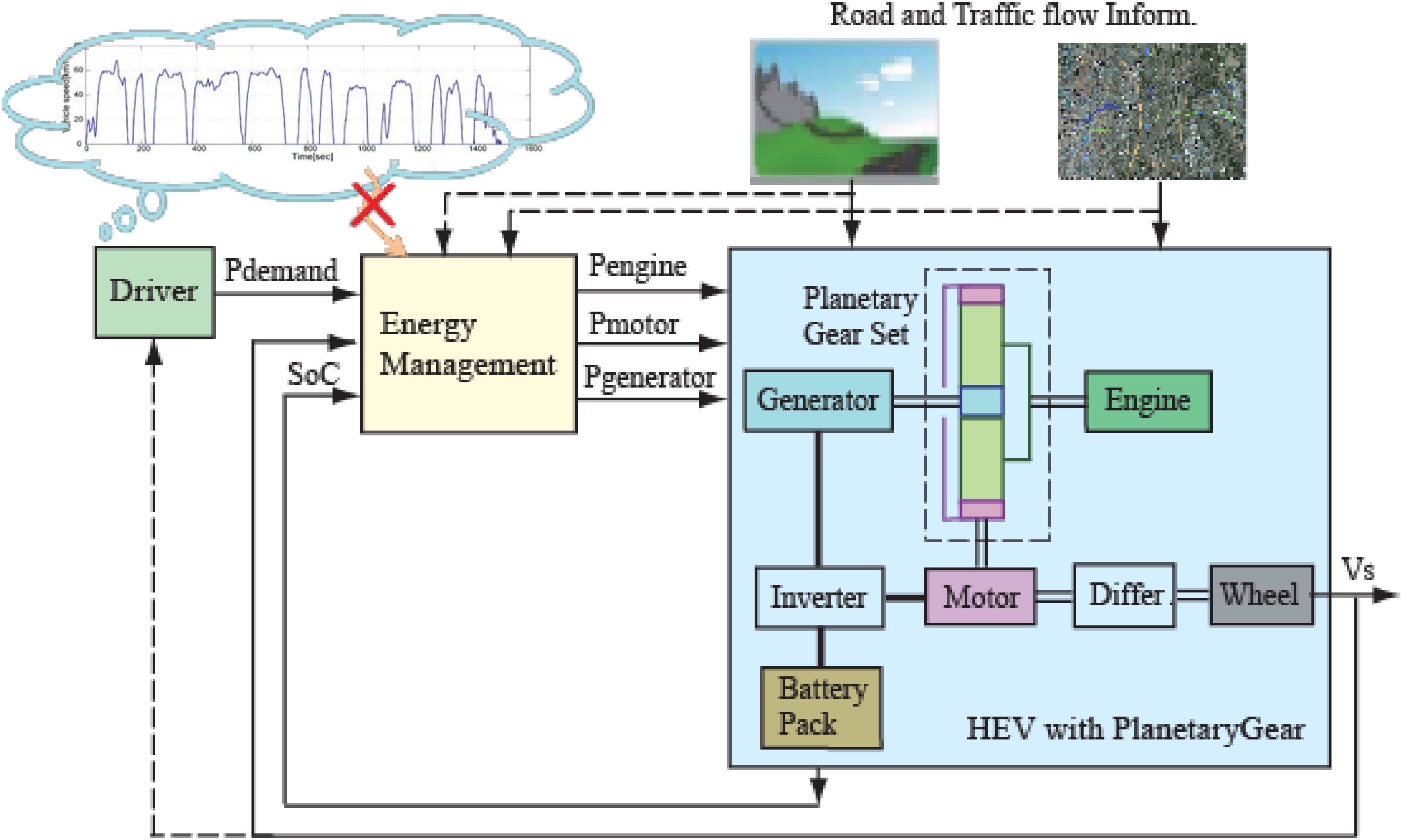
The powertrain configuration of the Toyota hybrid system (THS) shown in Figure 1 is considered. As is shown, the powertrain architecture consists of a planetary gear set, three power sources including an internal combustion engine, a motor and a generator, and a battery pack. Three nodes of the planetary gear, the sun gear, the carrier gear, and the ring gear, are connected to the generator, engine and motor, respectively.

Figure 1. Powertrain configuration of hybrid electric vehicle.

Figure 1. Powertrain configuration of hybrid electric vehicle.

For power split task, the power flow paths in the following basic operation modes should be one of primary concerns:

(1)

Motor alone propels the vehicle. The motor can be powered by either the battery or the generator that transforms the mechanical power generated by the engine into the electrical power. i.e., the driver propelling power demand P_trac,dem, and battery discharge power P_batt,dis can be written as:

P_trac,dem = P_m = T_mω_m

(1)

P_batt,dis = P_m / η_m

(2)

where P_m, T_m, ω_m are the motor power, torque and speed, respectively. η_m is the motor efficiency, which is generally a function of the motor torque and speed.

(2)

Engine alone propels the vehicle, in which the mechanical power generated by the engine is transmitted to the vehicle from the carrier gear directly to the ring gear connected to the final drive. Meanwhile, the excess engine power can be transformed to the electrical form through the generator and then pumped into the battery. i.e., the driver propelling power demand P_trac,dem, and battery charge power P_batt,ch can be written as:

P_trac,dem = T_rω_r = T_rω_m

(3)

P_batt,ch = η_gP_g = η_gT_gω_g

(4)

where P_g, T_g, ω_g are the generator power, torque and speed, respectively. η_g is the generator efficiency, generally, which also is a function of its torque and speed. T_r, ω_r are the ring gear torque and speed, respectively.

(3)

Engine and motor jointly propel the vehicle, i.e., the demand power of the vehicle is provided by both engine and motor. However, the motor may be powered by the generator, besides by the battery. i.e., the driver propelling power demand P_trac,dem, and battery power P_batt can be written as:

P_trac,dem = T_rω_r + T_mω_m = (T_r + T_m)ω_m

(5)

P_batt = η_gP_g + P_m / η_m = η_gT_gω_g + T_mω_m / η_m

(6)

(4)

The vehicle experiences braking. Here we only consider when the demanded braking power is less than the maximum regenerative braking power that the motor can supply. Then, the motor is controlled to function as a generator to produce a braking power that equals the commanded braking power. i.e., the driver braking power demand P_brak,dem, and battery charge power P_batt,ch can be written as:

P_brak,dem = T_mω_m

(7)

P_batt,ch = η_mP_m = η_mT_mω_m

(8)

Accordingly, the driver power demand P_dem and the battery power P_batt can be represented as:

P_dem = T_eω_e + T_gω_g +T_mω_m

(9)

(10)

where P_batt > 0 indicates the battery is discharging and P_batt < 0 means charging state. P_m < 0, P_g < 0 represent generating states and P_m > 0, P_g > 0 represent motoring states, and:

Obviously, the usage of the planetary gear set results in the redundancy of power flow paths. This merit, together with battery storage capacity and power sources with suitable size, can help to design the energy management strategy for improving the fuel economy while meeting the overall vehicle power demand.

For the planetary gear unit, as a result of the mechanical connection through gear teeth meshing, the speeds of the sun gear ω_s, ring gear ω_r, and carrier gear ω_c, have the relationship:

(R_r + R_s)ω_c = R_rω_r + R_sω_s

(11)

where R_r, R_s are the radii (or number of teeth) of the ring gear and sun gear respectively.

Neglecting the energy losses in steady-state operation, the torques acting on the sun gear T_s, ring gear T_r, and carrier gear T_c have the relationship:

(12)

And the dynamics with respect to the rotational speeds of generator, engine and motor can be described as follows, respectively:

(13)

(14)

(15)

where J_g, J_e, J_m, are the inertia of the generator, the engine, and the motor, respectively. T_trac is the torque on the axle of the differential gear, and g_f is the final differential gear ratio.

Moreover, assuming that the connecting shafts are rigid, the following speed relationships hold:

(16)

where v is the vehicle velocity, and R_tire is the radius of the tire.

The dynamics of the vehicle velocity is modeled as:

(17)

where M is the vehicle mass, and g denotes the gravity acceleration; η_f is the transmission efficiency of differential gear; T_br the friction brake torque; μ_r coefficient of rolling resistance; ρ air density; A frontal area of vehicle; C_d drag coefficient; and θ road angle (grading).

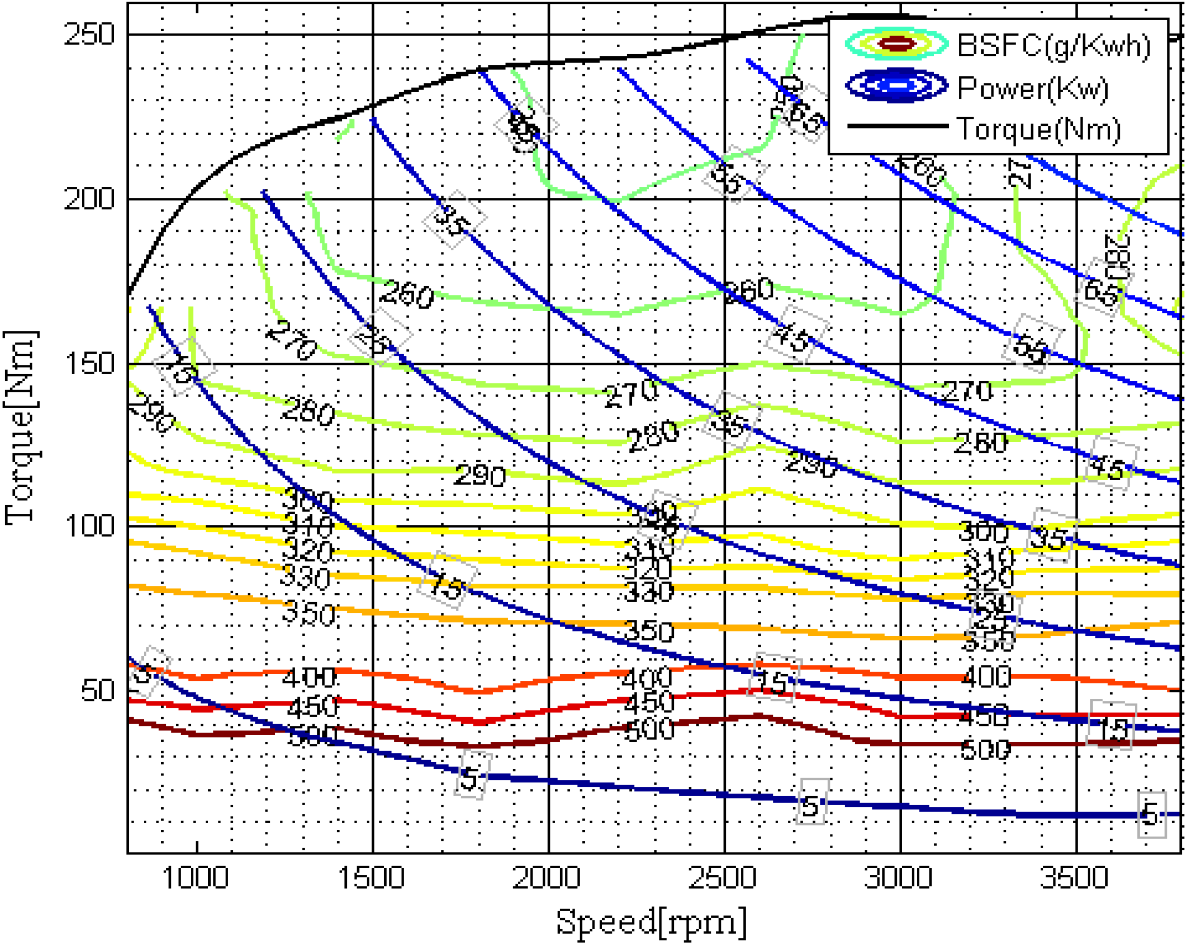
For power splitting with fuel economy, the break specific fuel consumption (BSFC (g/kWh)) should be an important parameter, which generally can be described by a map of the engine torque and speed. For example, the BSFC map of a certain gasoline engine is shown in Figure 2. The fuel consumption is measured by the fuel mass flow rate ṁ_f (g/s), which is defined as follows:

ṁ_f = BSFC × P_e × 10⁻⁵ / 36

(18)

Similarly, electricity consumption is evaluated by the instantaneous rate of change of the battery’s internal energy, i.e.:

P_elec = V_ocI_batt = −V_ocI_battSȯC

(19)

where V_oc, I_batt, Q_batt, SoC are battery open-circuit voltage, cuurent, maximum charge capacity, and state of charge, respectively. The dynamics of battery SoC can be represented by:

(20)

where R_b is battery internal resistance. Both V_oc and R_b are functions on battery SoC, which can be obtained through curve-fitting a predefined map.

Figure 2. BSFC map of a gasoline engine.

Figure 2. BSFC map of a gasoline engine.

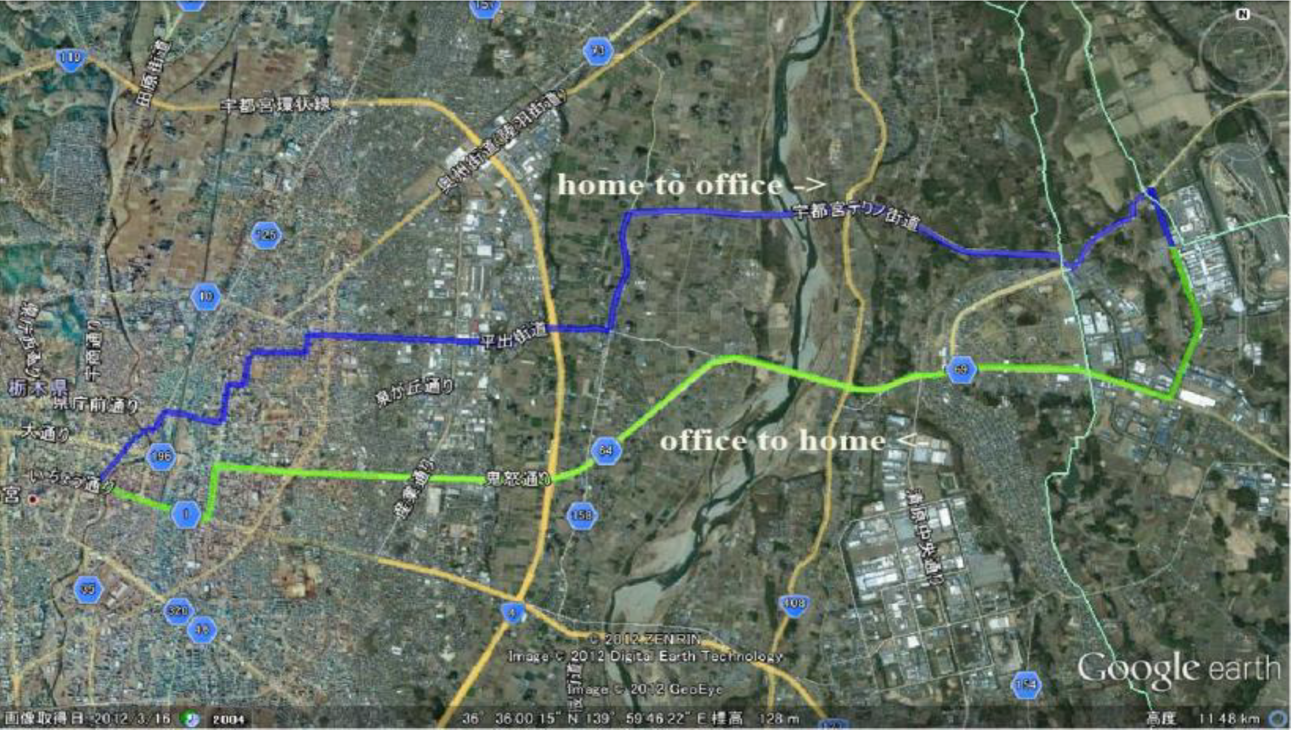
2.2. Traffic Information

For commuter vehicles, a certain amount of traffic-environment information can be available, such as traffic speed and road slope. Although a private commuter car does not have a fixed route like a public bus, according to the empirical evidence, a regular route can mostly be determined after a long run. On this regular route, information about the position for every crossing, intersection, speed bump, and traffic light, together with the road slope of each segment, is completely known, while, uncertainty and randomness still exists in the traffic flow information even if the departure time of the commuter car is usually during rush hour.

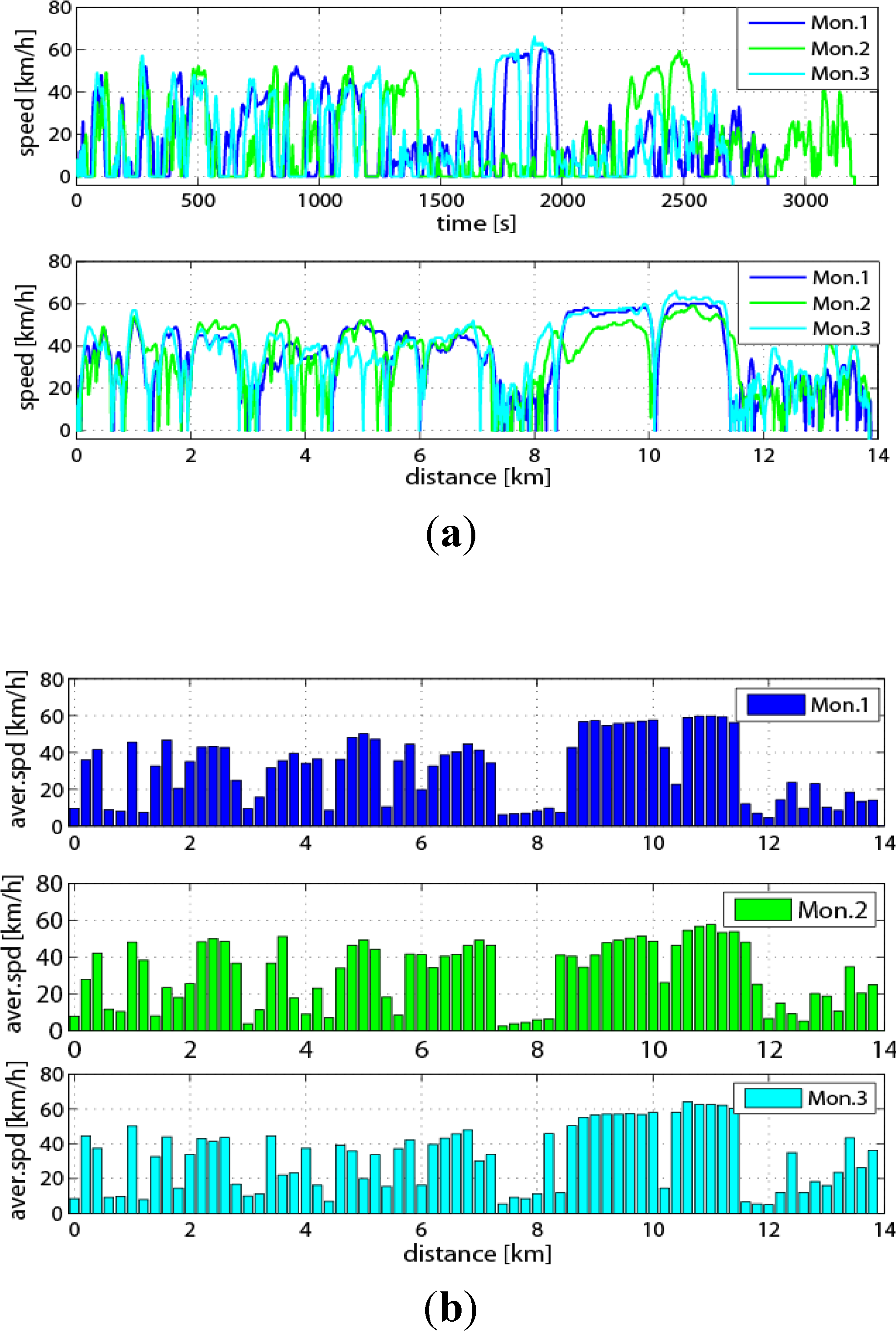
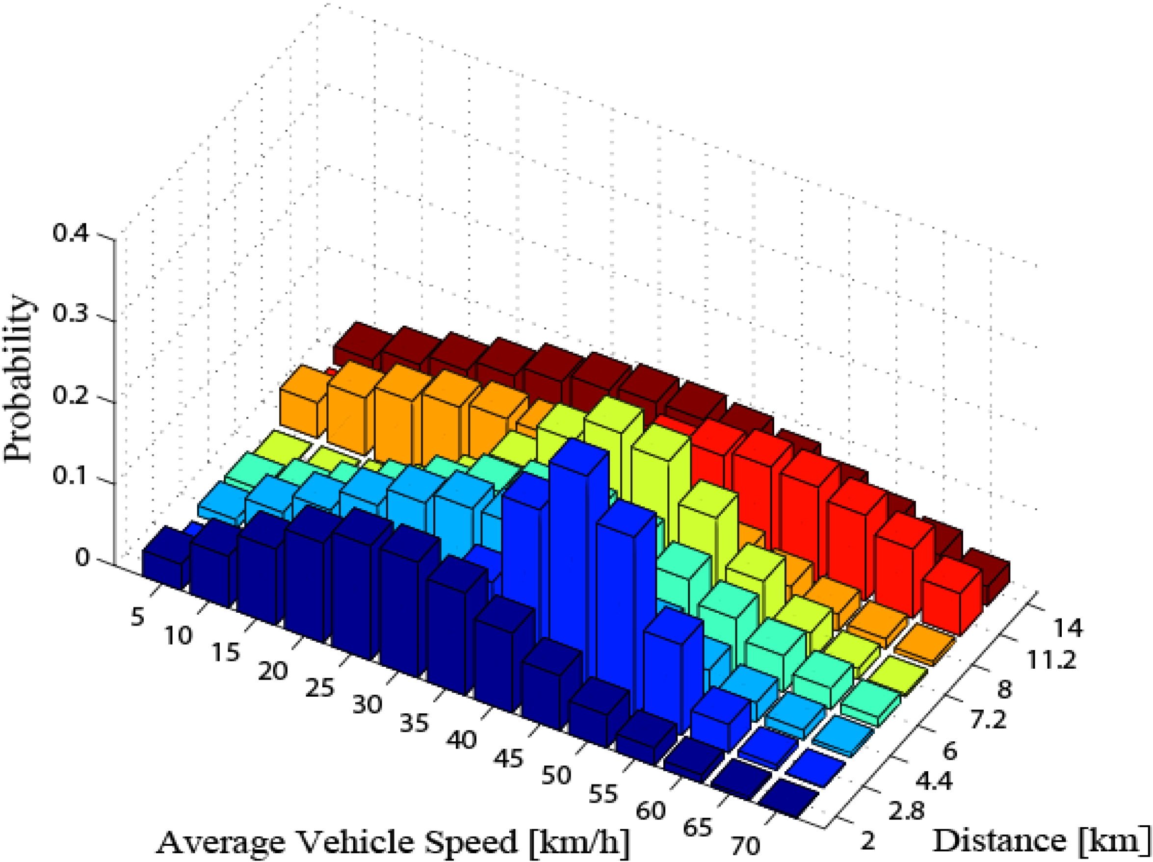
For example, on the same route, the instantaneous speeds during rush hour are still different for different workdays in the same week, as shown in Figure 3a, and for the same workday in the different weeks, as shown in Figure 4a. However, the statistical characteristics of the traffic speed can be captured in a certain segment of the route. It can be seen from Figure 3b and Figure 4b that the distribution of the average speed based on the trip distance in a certain segment has similar statistical characteristics, such as the segment-1 from 0 to 2 km, the segment-j from 6.0 to 7.2 km. Accordingly, the regular route can be divided into a number of segments according to the similar statistic characteristic in each segment.

Admittedly, it is complex to extract the characteristics of traffic information, which includes many characteristic parameters, such as roadway type, driving mode and driving trend. However, it should be noted that the characteristics is generally extracted in terms of the intended use. The study purpose of this paper is to determine the energy management strategy, whose effectiveness is influenced by the driving conditions as little as possible, so as to achieve the performance improvement on the fuel economy and charge sustenance of hybrid electric vehicles in real driving. To this end, the statistical characteristics in traffic speed profile are captured with a stochastic model, which in turn can be used to generate an optimal control policy to minimize, on average, automotive vehicle fuel-electricity consumption. The details will be described in next Section.

Figure 3. Traffic speed information on Monday, Wednesday, Friday in one week. (a) The instantaneous speed vs. time and vs. distance; (b) the average speed vs. distance.

Figure 3. Traffic speed information on Monday, Wednesday, Friday in one week. (a) The instantaneous speed vs. time and vs. distance; (b) the average speed vs. distance.

Figure 4. Traffic speed information on Mondays in three weeks. (a) The instantaneous speed vs. time and vs. distance; (b) the average speed vs. distance.

Figure 4. Traffic speed information on Mondays in three weeks. (a) The instantaneous speed vs. time and vs. distance; (b) the average speed vs. distance.

2.3. Problem Formulation

The energy management problem will be investigated for the hybrid electric commuter vehicle described above. Certainly, the objective of energy management is also normally as much as possible to reduce the fuel consumption while satisfying the battery charge-sustaining constraints and the overall vehicle power demands.

It should be noted that the hybrid powertrain utilized here is a normal hybrid electric vehicle, not a plug-in type. Therefore, like in most hybrid electric vehicles (HEVs), a charge sustaining strategy is adopted, which implies that the electricity used during a battery discharge phase must be replenished at a later phase using the fuel from the engine (either directly or indirectly through a regenerative path), such that at the end of driving path, the battery state of charge (SoC) should remain within a prescribed range, rather than achieve the minimum limit value.

Figure 5. System configuration of the HEV with energy management using traffic information.

Figure 5. System configuration of the HEV with energy management using traffic information.

Furthermore, the emphasis of this paper is on investigating the use of traffic information rather than the reference driving cycle to manage the distribution of the demand power so as to guarantee the effectiveness of energy management in real driving. Figure 5 illustrates the system configuration of this kind of HEV. Therefore, the following missions will be accomplished in the design of energy management of this paper:

(1)

The statistical characteristic of the traffic speed profile information from the collected data is modeled for achieving and generating scenarios in the stochastic approach for energy management.

(2)

The design objective of the energy management is achieved, i.e., the statistical characteristic, rather than the reference driving cycle, is utilized to design energy management strategy so as to guarantee the optimization for fuel-electricity consumption, the battery state-of-charge maintained within some specified limits, and the power demand for drivability of hybrid electric vehicles irrespective of real traffic flow and driving conditions.

(3)

The compromises, between the benefit of reduced trip information and computing requirement, and the expense of reduced performance, are considered in the design of the control policy.

3. Energy Management Based on SDP

By taking the statistics of traffic speed profiles in the driving route into account, a stochastic approach for the energy management is adopted to optimize fuel-electricity consumption in an average sense. The charge sustaining goal is incorporated into the control design process through the control strategy based on the SDP to obtain a time-invariant control policy for the SoC.

3.1. Traffic Information Modeling

As indicated already in the problem description, the approach in this paper is stochastic modeling of driving cycle by using collected speed data in urban traffic. The various steps involved in the modeling work will be described in more detail below.

The construction of traffic speed statistics is based on the actual commute driving speed data collected along the regular route as shown in Figure 6, which is provided by JSAE-SICE benchmark problem 2, see [19].

Figure 6. The actual route profile.

Figure 6. The actual route profile.

The data set included commuter driving between the user’s home and office on weekdays and city driving for shopping on weekends during three weeks, where the commute driving only is stop and go type driving, not including freeways. Here we only consider how to use the traffic information to deal with the energy management problem for the commute driving, moreover, the difference of the traffic information between the going and the returning route is taken into account, thus the 15 days commute driving speed data in the going route (from home to office) are sampled to model the statistics of the traffic speed profile, and further utilized to formulate the stochastic control problem for the energy management. We used the 15 days of driving data from home to office in this study to determine the probability distribution as follows:

(1)

To calculate the average speed according to a distance of 200 m to obtain the average speed profile vs. the distance for the adequate speed profile sampled, which on Monday, Wednesday and Friday in one week has been shown in Figure 3.

(2)

To divide the total distance into a number of segments, according to the similar statistics of the averaged speed vs. distance observed in a certain segment for all sampled day data. In this study, the total distance is 14 km and divided into eight segments, in which the distance of the each segment is:

L = [0–2 km, 2–2.8 km, 2.8–4.4 km, 4.4–6 km, 6–7.2 km, 7.2–8 km, 8–11.2 km, 11.2–14 km]

(3)

To determine the probability distribution of the average speeds for each segment. Each segment has a different probability distribution of the average speed profile, but, it can be assumed that its probability distribution is invariant in the segment and fitted to the normal distribution.

By using nearest-neighbor quantization, the averaged speeds are quantized as:

v = [5, 10, 15, 20, 25, 30, 35, 40, 45, 50, 55, 60, 65, 70] km/h

The probability distribution of the quantized speed can be estimated by the maximum likelihood estimation method. The corresponding mean μ and standard deviation σ are estimated according to the all sampled data of the 15 days in the i-th segment as:

(21)

where are the estimate of the mean and deviation, respectively. x_j is the j-th sampled data of the total sampled data n in the i-th segment.

The probability distribution of the i-th segment can be estimated through the following normal cumulative distribution function:

(22)

Figure 7 shows example of obtaining the probability distribution Prob₁(v) in the first segment. Similarly, the probability distribution Prob_j(v), j = 1,2,···,8 in each segment of the driving route can be obtained, which is shown in Figure 8.

Figure 7. Example of obtaining the probability distribution.

Figure 7. Example of obtaining the probability distribution.

Figure 8. Probability distribution in each segment of the driving route.

Figure 8. Probability distribution in each segment of the driving route.

The approach to the energy management in this paper is to model a stochastic process based on the traffic information model, and to formulate a stochastic optimal problem with infinite horizon, further, to derive an invariant state feedback optimal control policy by the policy iteration of the SDP.

3.2. Stochastic Process Model and Optimization Problem

Considering the objective of energy management and the feature of SDP, in the constructed stochastic process model, only the battery SoC is regarded as system state, the motor torque T_m and the generator speed ω_g are control inputs, and the average vehicle speed in term of distance as stochastic disturbance. Meanwhile, for obtaining control laws T_m and ω_g by the discrete stochastic dynamic programming, the battery dynamics Equation (20) is rewritten in the following discrete form:

SoC_k+1 = f(SoC_k,ω_g,k,T_m,k,v_k) = SoC_k + ΔSoC_k

(23)

where:

P_batt(ω_g,k,T_m,k,v_k) is described as:

(24)

and P_dem is also the average power, which can be determined by:

(25)

Consequently, for the each segment in the regular route, the control-oriented model of HEVs is described as a discrete stochastic process with stationary Markov chain. Where the system state is x_k = SoC_k, the control input is u_k = (ω_g,k,T_m,k) and the stochastic disturbance is w_k = v_k. And x_k ∈ S, u_k ∈ C, v_k ∈ D,S,C,D are finite sets and S = {1, 2, ···, s}. u_k is constrained to take values in a given nonempty subset U(x_k) of C, i.e., u_k ∈ U(x_k), ∀x_k ∈ S. The random disturbances w_k has identical statistics [20]. Furthermore, the stochastic optimization problem is formulated as follows:

The optimal control policy in the each segment can be extracted by minimizing the cost function:

(26)

subject to the system state Equation (23) and the constraints:

SoC_min ≤ SoC ≤ SoC_max, ω_emin ≤ ω_e ≤ ω_emax, ω_gmin ≤ ω_g ≤ ω_gmax,
T_emin ≤ T_e ≤ T_emax, T_mmin ≤ T_m ≤T_mmax, P_e ≤ P_erated, P_m ≤ P_mrated, P_g ≤ P_grated

where α is a discount factor and 0 < α < 1. The cost functional g is defined as the sum of the fuel consumption and electricity consumption g = g_fuel,comp + g_elec,comp, which are expressed as:

g_fuel,comp (ω_g,k,v_k)=ṁ_f,k · H_l · ΔL/v_k = BSFC_k · P_e,k · H_l· 10^-3 · ΔL/v_k

(27)

g_elec,comp (SoC_k,ω_g,k,T_m,k,v_k)= γ · P_elec,k · ΔL/v_k · 3.6 · 10⁻³

(28)

where BSFC_k is utilized in term of the following formula, which is a map fitting by the least-square algorithm:

(29)

and:

(30)

It should be noted that the Equation (23) is of discrete vs. a small distance ΔL, and v_k ,ω_g,k,T_m,k represent the average measure of the vehicle speed, generator speed and motor torque at the end of the interval ΔL.

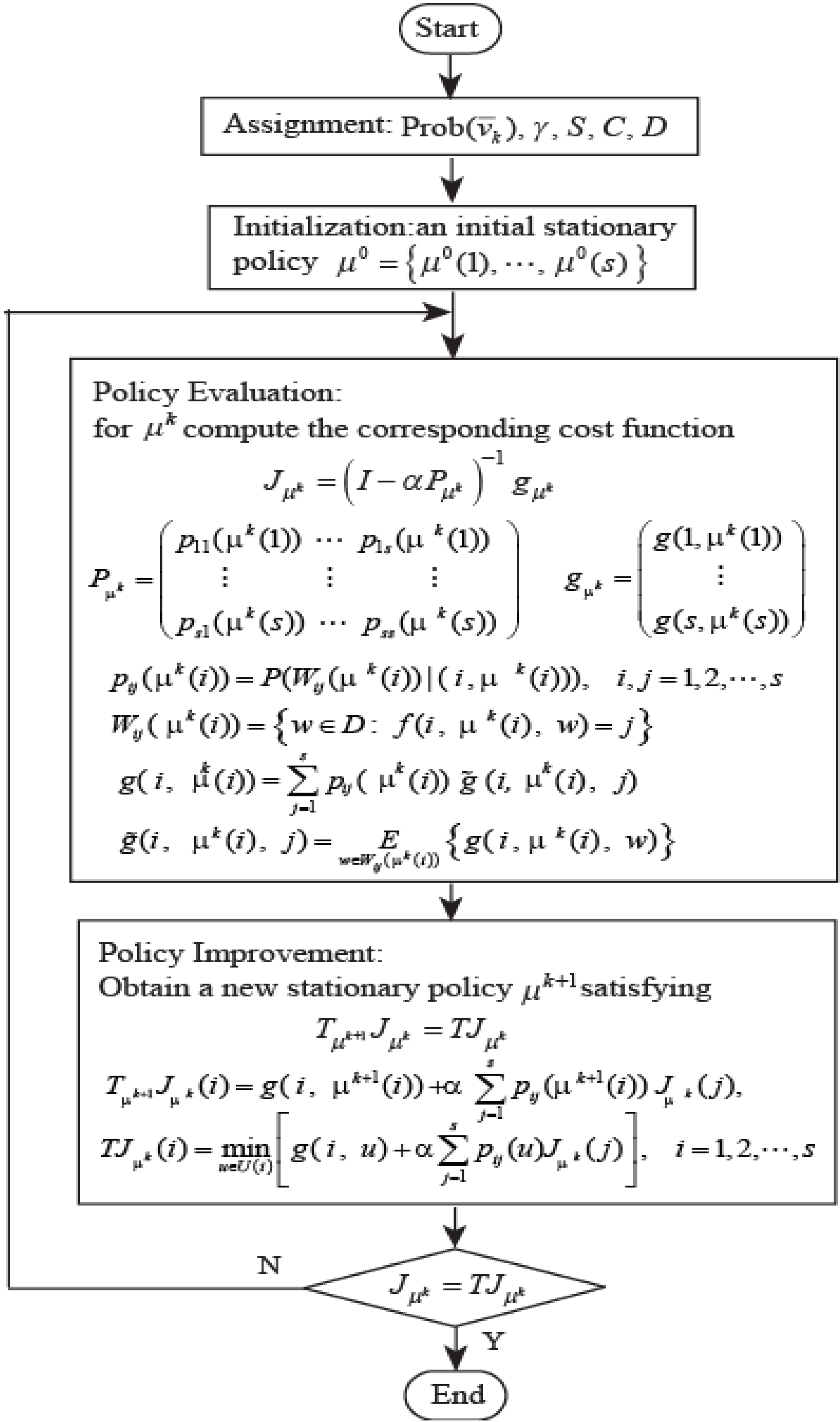
3.3. Control Policy Iteration of SDP for Optimal Solution

The SDP problem is solved through a policy iteration algorithm, which consists of a policy evaluation step and a policy improvement step. This algorithm is solved iteratively until the cost function converges. The algorithm procedure is shown in Figure 9.

Figure 9. The procedure of the control policy iteration.

Figure 9. The procedure of the control policy iteration.

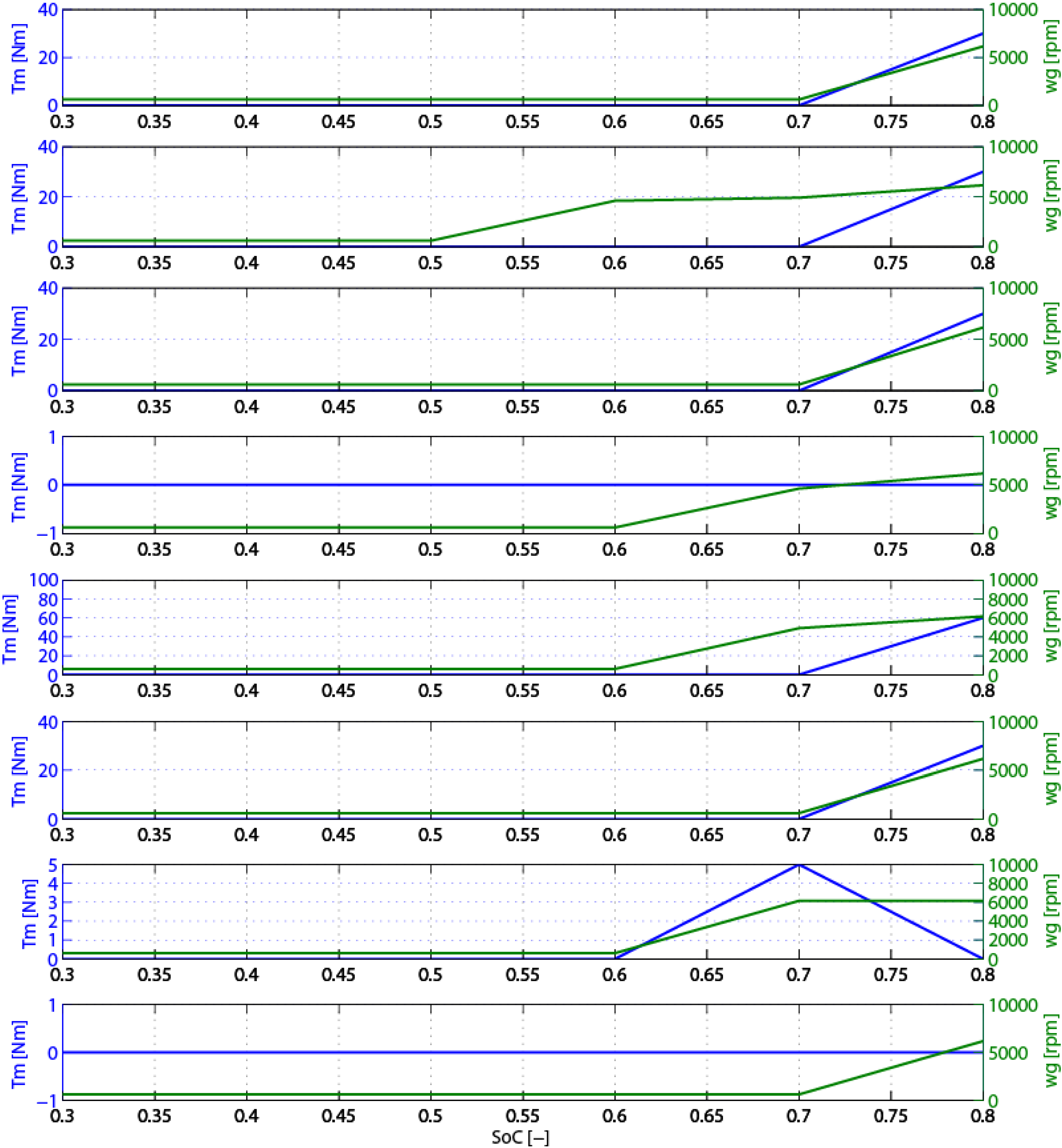
This process is repeated until converges within a selected tolerance level. The control policy generated is time-invariant and causal and has the form of nonlinear full-state feedback laws. An example of the control law maps (SoC, ω_g) and (SoC, T_m) are shown in Figure 10, notice that the accuracy is limited by the grid size on each state.

It should be noted that the control policy obtained from the above SDP-policy iteration algorithm only applies to the basic operation modes of powertrain. Furthermore, note that through determining the generator speed ω_g and the motor torque T_m, the demand torques T_er, T_gr, T_mr for the power sources can be obtained. Since engine can be controlled at its optimal operating area as long as it is operating, which indicates the engine torque T_e can be a function on the engine speed ω_e through the curve-fitting the optimal torque operating line. Consequently, combining the determined ω_g and the vehicle speed can derive the engine speed ω_e, and then the demand torque for engine T_er is obtained. Meanwhile, combining the determined T_mr and the traction power demand can derive the demand torque for generator T_gr.

Figure 10. Control policy in the regular route.

Figure 10. Control policy in the regular route.

4. Simulation Validation and Observation

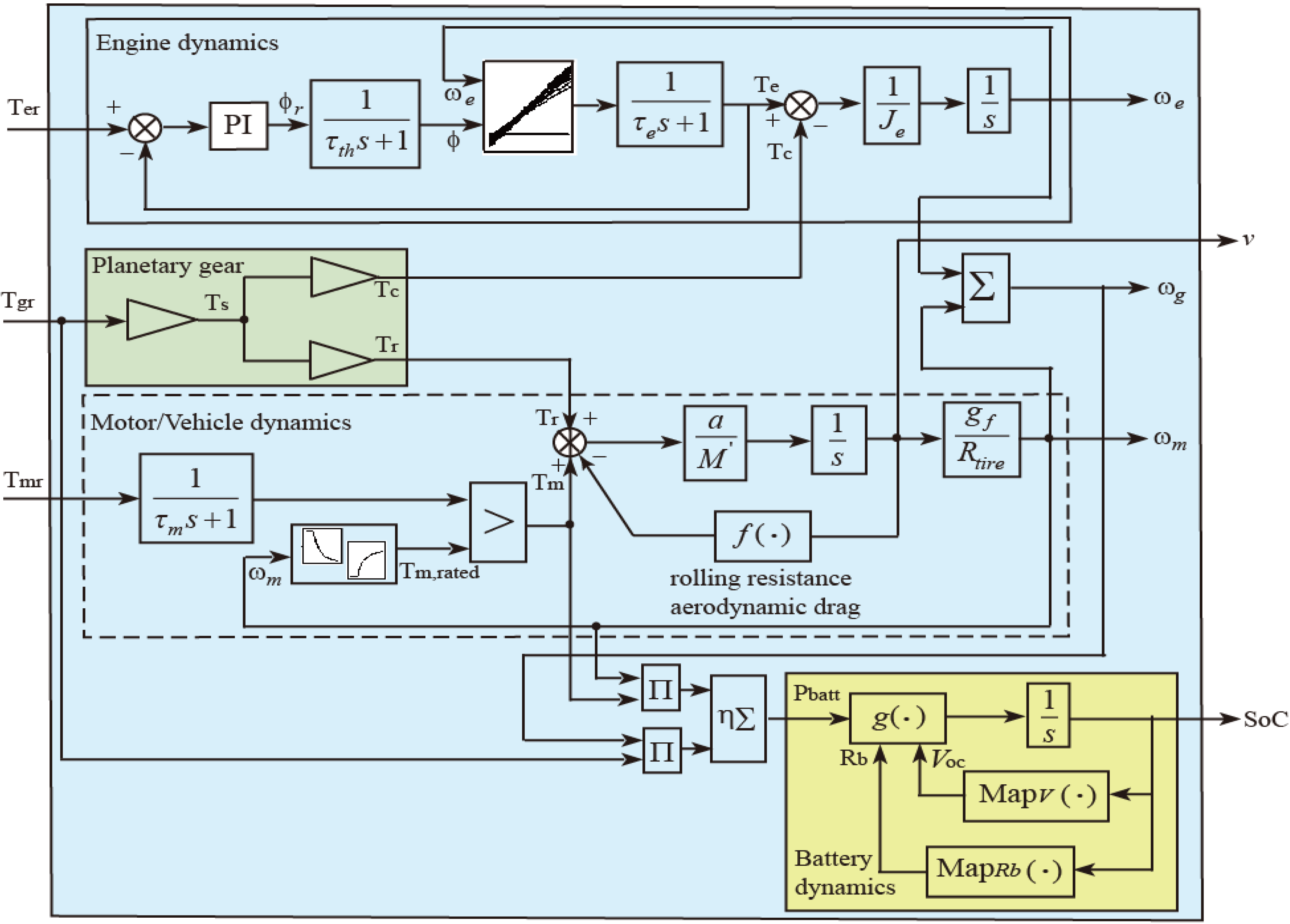
Simulation of the presented energy management strategy for the HEV is executed to verify the effectiveness for the fuel economy, battery charge-sustaining constraints and the power demand for drivability. In simulation, the HEV system with the energy management is constructed as shown in Figure 11, where a model resembling a real engine includes the dynamics of electric throttle, the process of the engine torque generation, the process of the start-up, and the limitations for the rated power, the maximum torque, the maximum speed, besides the dynamics of the rotational speed Equation (14) and the fuel consumption Equation (18) and the BSFC map as Figure 2. The model resembling real motor consists of the dynamics of the rotational speed Equation (15), the dynamical response of torque and the limitations for the maximum torque, the maximum speed. The model resembling real battery is comprised of the SoC nonlinear dynamical description Equation (20) with Equation (10), maps of battery open-circuit voltage and internal resistance. The vehicle model and the planetary gear are constructed as the description Equations (17) and (11)–(12), respectively, The connecting shafts are assumed to be rigid and described as the relationship Equation (16). This suite of subsystems created in Matlab/Simulink is shown in Figure 12.

Figure 11. Schematic of HEV system with torque-split control in simulation.

Figure 11. Schematic of HEV system with torque-split control in simulation.

Figure 12. Schematic diagram of model resembling real powertrain in simulation.

Figure 12. Schematic diagram of model resembling real powertrain in simulation.

The physical parameters used of the HEV model are listed in Table 1 [19]. It should be noted that the motor efficiency is adopted as a constant coefficient rather than a map of the motor speed and torque since the used physical parameter values in simulation are from the GT-Suite HEV model provided by Dr. Yuji Yasui, Honda R&D Co., where the EM efficiency only is a constant.

Table 1. Basic parameters of the HEV powertrain used in simulation.

Notation	Meaning	Value (Unit)
M	Vehicle mass	1460 (kg)
ρ	Air density	1.293 (kg/m3)
Cd	Air drag coefficient	0.33
A	Frontal area of vehicle	3.8 (m2)
μ	Coefficent of rolling resistance	0.015
gf	Final differential gear ratio	4.113
Rtire	Radius of the tire	0.2982 (m)
Je	Inertia of the engine crankshaft	0.16 (kg·m2)
Jm	Inertia of the motor	0.035 (kg·m2)
Jg	Inertia of the generator	0.0265 (kg·m2)
ε	planetary gear ratio	0.3846
ηm	Efficiency of EM as motor	0.8301
ηg	Efficiency of EM as generator	0.876
Qmax	Battery maximum charge capacity	6.5 (Ah)

Table 1. Basic parameters of the HEV powertrain used in simulation.

Notation	Meaning	Value (Unit)
M	Vehicle mass	1460 (kg)
ρ	Air density	1.293 (kg/m3)
Cd	Air drag coefficient	0.33
A	Frontal area of vehicle	3.8 (m2)
μ	Coefficent of rolling resistance	0.015
gf	Final differential gear ratio	4.113
Rtire	Radius of the tire	0.2982 (m)
Je	Inertia of the engine crankshaft	0.16 (kg·m2)
Jm	Inertia of the motor	0.035 (kg·m2)
Jg	Inertia of the generator	0.0265 (kg·m2)
ε	planetary gear ratio	0.3846
ηm	Efficiency of EM as motor	0.8301
ηg	Efficiency of EM as generator	0.876
Qmax	Battery maximum charge capacity	6.5 (Ah)

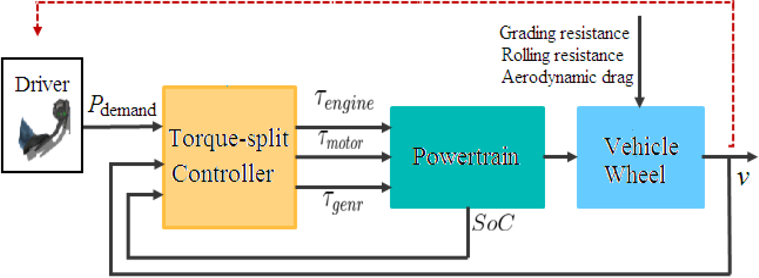
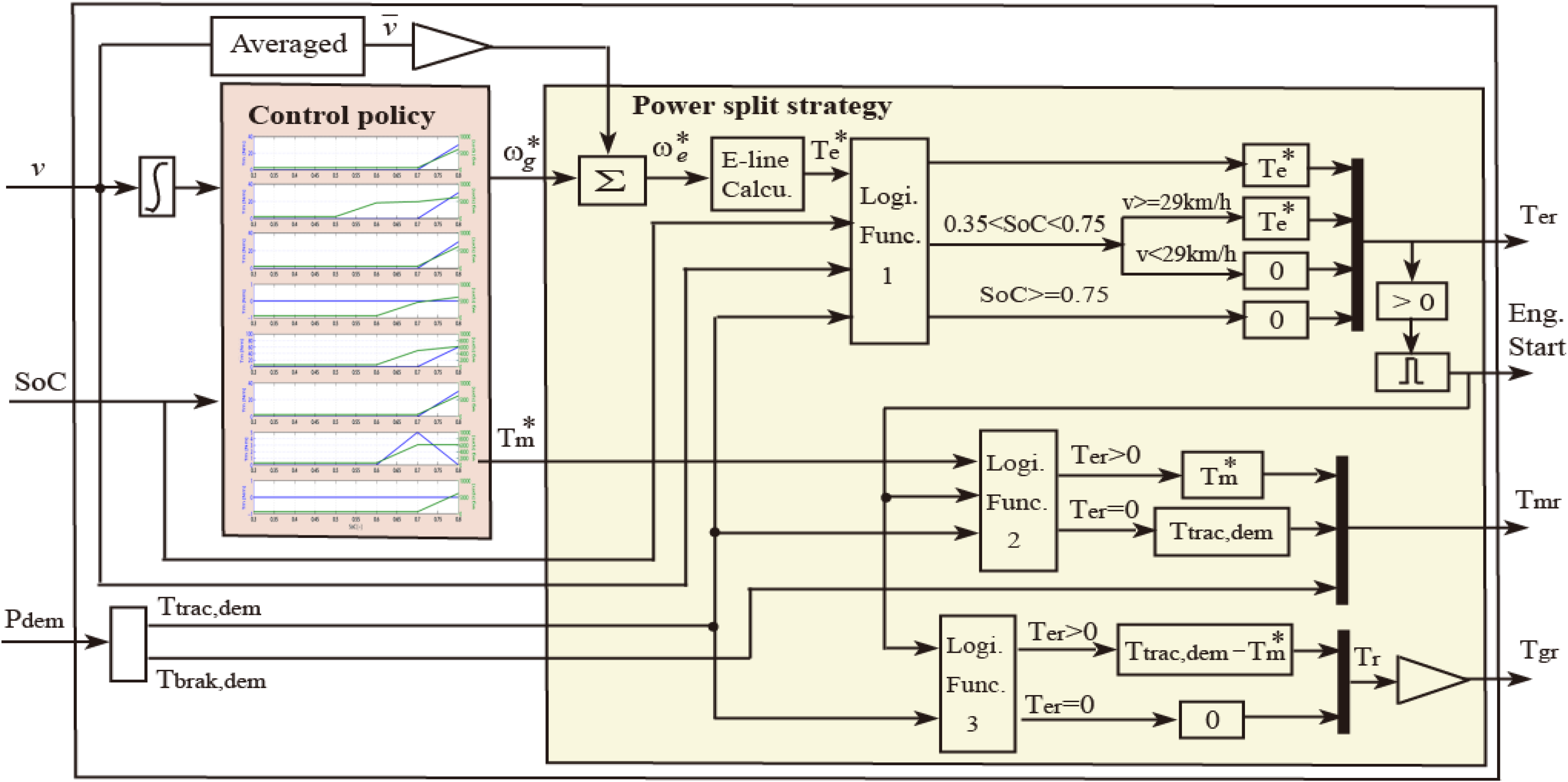
Furthermore, the driver’s throttle and brake pedal commands are interpreted as a power demand to be satisfied by the powertrain. The driver power demand is an input to the torque-split controller, the real-time implementation of the designed SDP-based energy management strategy. The torque-split controller is comprised of the component obtaining control policy command ω_g^*, T_m^* from SDP-based management strategy, the component transforming the control policy command ω_g^*, T_m^* into the torque demands T_er, T_gr, T_mr distributed to the power sources, and some logical strategies in terms of the limitations for thermal and/or mechanical conditions as well as a whole operation range of boundary conditions. The schematic diagram of the torque-split controller is shown in Figure 13.

For purposes of validating the effectiveness of the proposed management strategy, the following three test cases are done on some driving cycles from the 15 days sample driving speed profile:

(1)

For sensory evaluation, the designed control policy shown in Figure 10, i.e., each segment in whole route has itself policy C_i → L_i, i = 1, 2, ···, 8, is executed in the HEV powertrain control system as shown Figure 11, to show the performance on the fuel-electricity consumption, charge sustenance, and drivability. Where the policy C_i → L_i, i = 1, 2, ···, 8, is called full-policy.

(2)

For comparative evaluation, a fixed single policy, such as C₂ is used for the whole route, i.e., the whole route only adopts the policy C₂ corresponding to the second segment L₂, executed in the HEV powertrain control system, to show the comparative performance on the fuel-electricity between the full-policy and the fixed policy C_i, i = 1, 2, ···, 8.

(3)

Similarly, a comparative evaluation is given by the results of driving speed profile only for a certain segment in the whole route. The comparison is made between the single policy corresponding to this segment and other single policies. For example, in terms of the driving speed profile in the segment L₃, comparison is given between the result of executing C₃ and that of executing C₇.

First, the third Monday driving speed profile and the first Wednesday driving speed profile are chosen as examples for Test case 1. The simulation results are shown in Figure 14 and Figure 15, respectively.

Figure 13. Schematic diagram of the torque-split controller in simulation.

Figure 13. Schematic diagram of the torque-split controller in simulation.

Figure 14. Result with the full-policy for the third Monday speed profile. (a) Vehicle speed, SoC and fuel-electricity consumption; (b) batter powery, demand power and engine, generator and motor power outputs; (c) engine, generator, motor speeds and their torques; (d) engine operating point densities.

Figure 14. Result with the full-policy for the third Monday speed profile. (a) Vehicle speed, SoC and fuel-electricity consumption; (b) batter powery, demand power and engine, generator and motor power outputs; (c) engine, generator, motor speeds and their torques; (d) engine operating point densities.

Figure 15. Result with the full-policy for the first Wednesday speed profile. (a) Vehicle speed, SoC and fuel-electricity consumption; (b) Batter power, demand power and engine, generator and motor power outputs; (c) Engine, Generator, motor speeds and their torques; (d) Engine operating point densities.

Figure 15. Result with the full-policy for the first Wednesday speed profile. (a) Vehicle speed, SoC and fuel-electricity consumption; (b) Batter power, demand power and engine, generator and motor power outputs; (c) Engine, Generator, motor speeds and their torques; (d) Engine operating point densities.

Then, 15 days sample driving speed profiles are chosen to perform test case 2 for comparative validation of the performance on fuel-electricity consumption. Table 2 shows the comparison between the full-policy and fixing single policy in 15 days driving speed profiles, where the result of full-policy is listed in the second column of Table 2, and the result of fixing single policy C_i, i = 1, 2, ···, 8 lie in the third column to the 10th column, respectively.

Table 2. Comparison of fuel-electricity consumption between the full-policy and single policy.

[km/L]	Full-poli	S1-poli	S2-poli	S3-poli	S4-poli	S5-poli	S6-poli	S7-poli	S8-poli
Mon1	30.9056	30.9056	30.8669	30.9056	30.9056	30.9056	30.9056	30.9056	30.9056
Mon2	28.3881	28.3881	27.5434	28.3881	28.3881	28.3881	28.3881	28.3881	28.3881
Mon3	33.7096	33.7096	33.7096	33.7096	33.7096	33.7096	33.7096	33.7096	33.7096
Tue1	25.5455	25.5455	25.4511	25.5455	25.5455	25.5455	25.5455	25.5455	25.5455
Tue2	19.8163	19.8163	16.2463	19.8163	19.2507	19.2163	19.8163	19.0881	19.8163
Tue3	20.7915	16.2526	15.2868	16.2526	21.0331	14.5505	16.2526	18.6054	20.2932
Wed1	22.1123	22.1123	19.0863	22.1123	22.1123	22.1123	22.1123	22.1123	22.1123
Wed2	28.8094	28.8094	28.6970	28.8094	28.8094	28.8094	28.8094	28.8094	28.8094
Wed3	26.7733	26.7733	26.7733	26.7733	26.7733	26.7827	26.7733	26.7827	26.7733
Thur1	26.6242	26.6242	26.3172	26.6242	26.6242	26.6242	26.6242	26.6242	26.6242
Thur2	22.3535	22.3535	19.2765	22.3535	22.3229	22.3207	22.3535	22.3124	22.3535
Thur3	25.5654	25.5654	25.5654	25.5654	25.5654	25.5654	25.5654	25.5654	25.5654
Fri1	30.4161	30.4161	17.5464	30.4161	30.4161	30.4161	30.4161	30.4161	30.4161
Fri2	23.3546	23.3546	20.8797	23.3552	23.2168	23.2069	23.3552	23.1733	23.3546
Fri3	25.5654	25.5654	25.5654	25.5654	25.5654	25.5654	25.5654	25.5654	25.5654
Averg	26.0487	25.7462	23.9208	25.7462	26.0159	25.5892	25.7462	25.8401	26.0155

Table 2. Comparison of fuel-electricity consumption between the full-policy and single policy.

[km/L]	Full-poli	S1-poli	S2-poli	S3-poli	S4-poli	S5-poli	S6-poli	S7-poli	S8-poli
Mon1	30.9056	30.9056	30.8669	30.9056	30.9056	30.9056	30.9056	30.9056	30.9056
Mon2	28.3881	28.3881	27.5434	28.3881	28.3881	28.3881	28.3881	28.3881	28.3881
Mon3	33.7096	33.7096	33.7096	33.7096	33.7096	33.7096	33.7096	33.7096	33.7096
Tue1	25.5455	25.5455	25.4511	25.5455	25.5455	25.5455	25.5455	25.5455	25.5455
Tue2	19.8163	19.8163	16.2463	19.8163	19.2507	19.2163	19.8163	19.0881	19.8163
Tue3	20.7915	16.2526	15.2868	16.2526	21.0331	14.5505	16.2526	18.6054	20.2932
Wed1	22.1123	22.1123	19.0863	22.1123	22.1123	22.1123	22.1123	22.1123	22.1123
Wed2	28.8094	28.8094	28.6970	28.8094	28.8094	28.8094	28.8094	28.8094	28.8094
Wed3	26.7733	26.7733	26.7733	26.7733	26.7733	26.7827	26.7733	26.7827	26.7733
Thur1	26.6242	26.6242	26.3172	26.6242	26.6242	26.6242	26.6242	26.6242	26.6242
Thur2	22.3535	22.3535	19.2765	22.3535	22.3229	22.3207	22.3535	22.3124	22.3535
Thur3	25.5654	25.5654	25.5654	25.5654	25.5654	25.5654	25.5654	25.5654	25.5654
Fri1	30.4161	30.4161	17.5464	30.4161	30.4161	30.4161	30.4161	30.4161	30.4161
Fri2	23.3546	23.3546	20.8797	23.3552	23.2168	23.2069	23.3552	23.1733	23.3546
Fri3	25.5654	25.5654	25.5654	25.5654	25.5654	25.5654	25.5654	25.5654	25.5654
Averg	26.0487	25.7462	23.9208	25.7462	26.0159	25.5892	25.7462	25.8401	26.0155

Where the unit [km/L] represents the moving distance (km) per liter fuel consumption for Unleaded Petrol No. 97. From both the 15 days driving speed profiles results in Table 2 and the averaged value in 15 days, it can be seen that in general the performance of full-policy is better than that of fixing a single policy even though there exists the case that not the longest distance [km] per liter fuel consumption for full-policy in individual driving speed profile exits. It follows that the proposed control strategy C_i → L_i can guarantee better fuel economy in an average sense than the control strategy with a fixed single policy in the whole route. It should be noted that the so-called summing-up in an average sense results not from the averaged value meanings, but rather the essential characteristic of the stochastic optimization. On the other hand, there is no doubt that the control policy of the stochastic optimization problem is dependent of the adequate statistical analysis. Thus, it is presumable that the appearance of not always optimal results from the question of whether the collected data is adequate enough for statistical analysis.

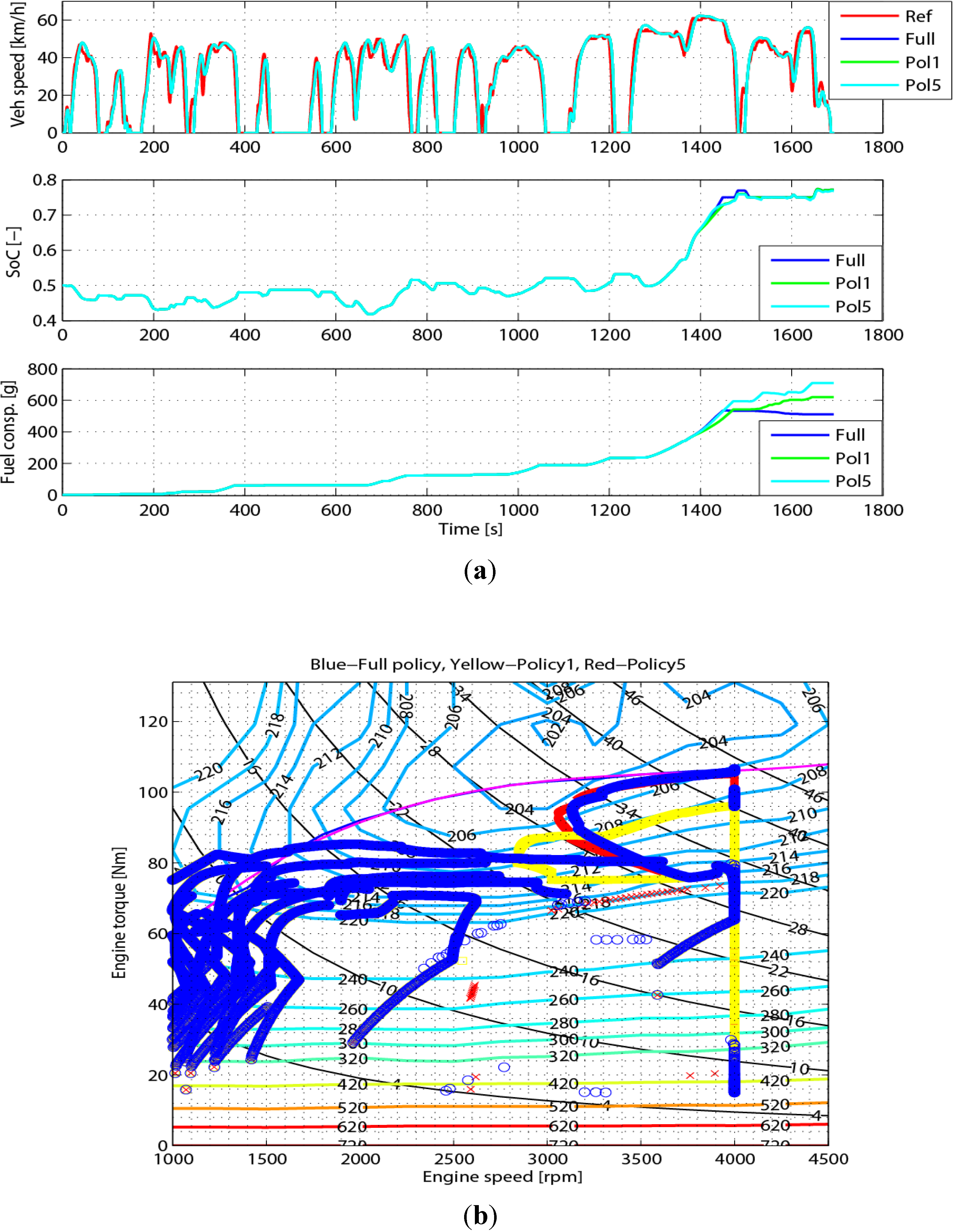
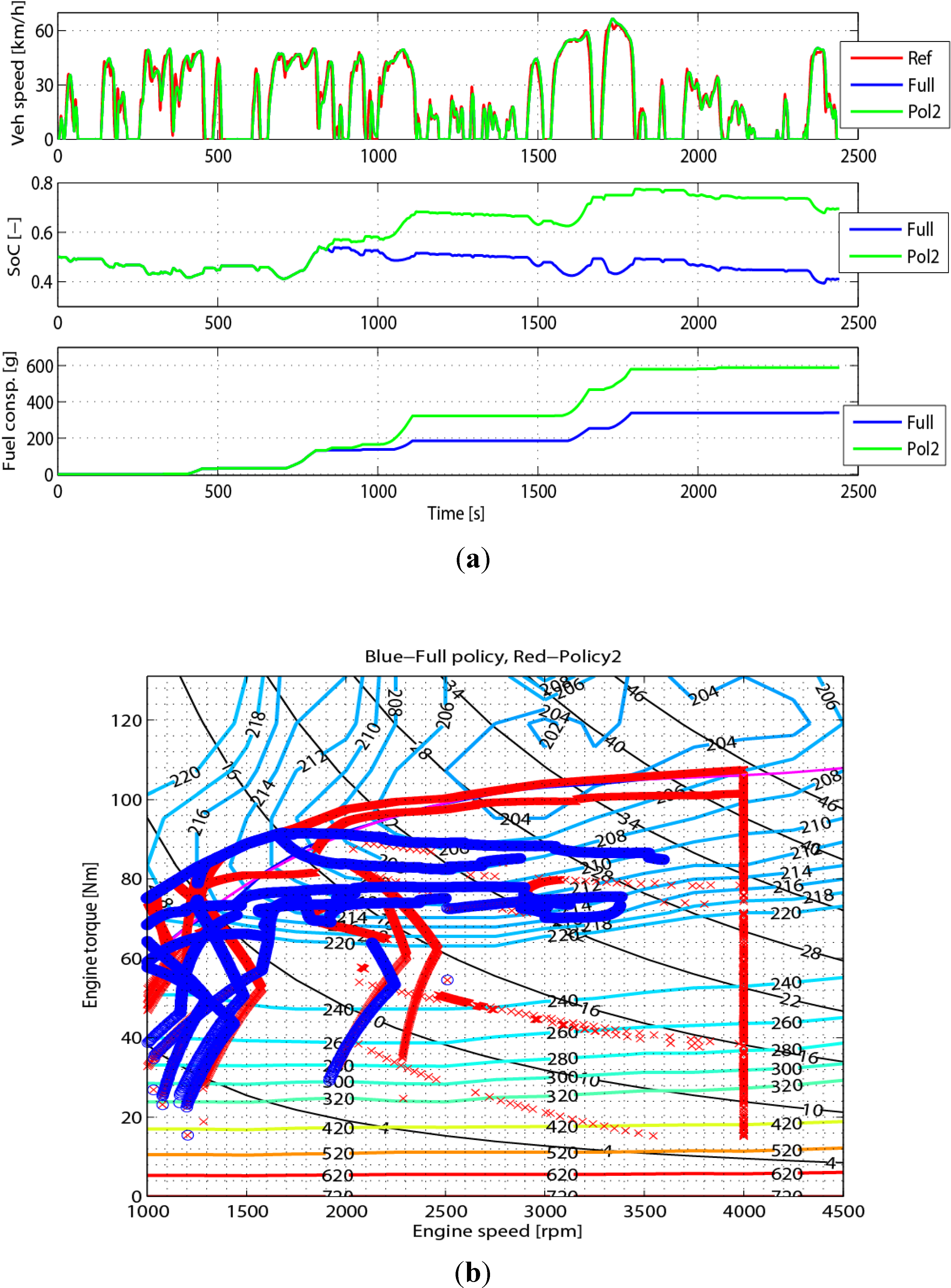
Meanwhile, for clear display, as examples, Figure 16 and Figure 17 also give the results of utilizing full-policy and a fixed single one in the third Tuesday and the first Friday speed profiles, respectively. These compared results of the SoC, the fuel consumption and the engine operating point density further demonstrate the effectiveness of the proposed energy management strategy on the improvement of fuel economy.

Figure 16. Comparison of the full-policy and a fixing single policy-1, single policy-5 in the third Tuesday speed profile. (a) Vehicle speed, SoC and fuel-electricity consumption; (b) engine operating point densities.

Figure 16. Comparison of the full-policy and a fixing single policy-1, single policy-5 in the third Tuesday speed profile. (a) Vehicle speed, SoC and fuel-electricity consumption; (b) engine operating point densities.

Figure 17. Comparison of the full-policy and a fixing single policy-2 in the first Friday speed profile. (a) Vehicle speed, SoC and fuel-electricity consumption; (b) engine operating point densities.

Figure 17. Comparison of the full-policy and a fixing single policy-2 in the first Friday speed profile. (a) Vehicle speed, SoC and fuel-electricity consumption; (b) engine operating point densities.

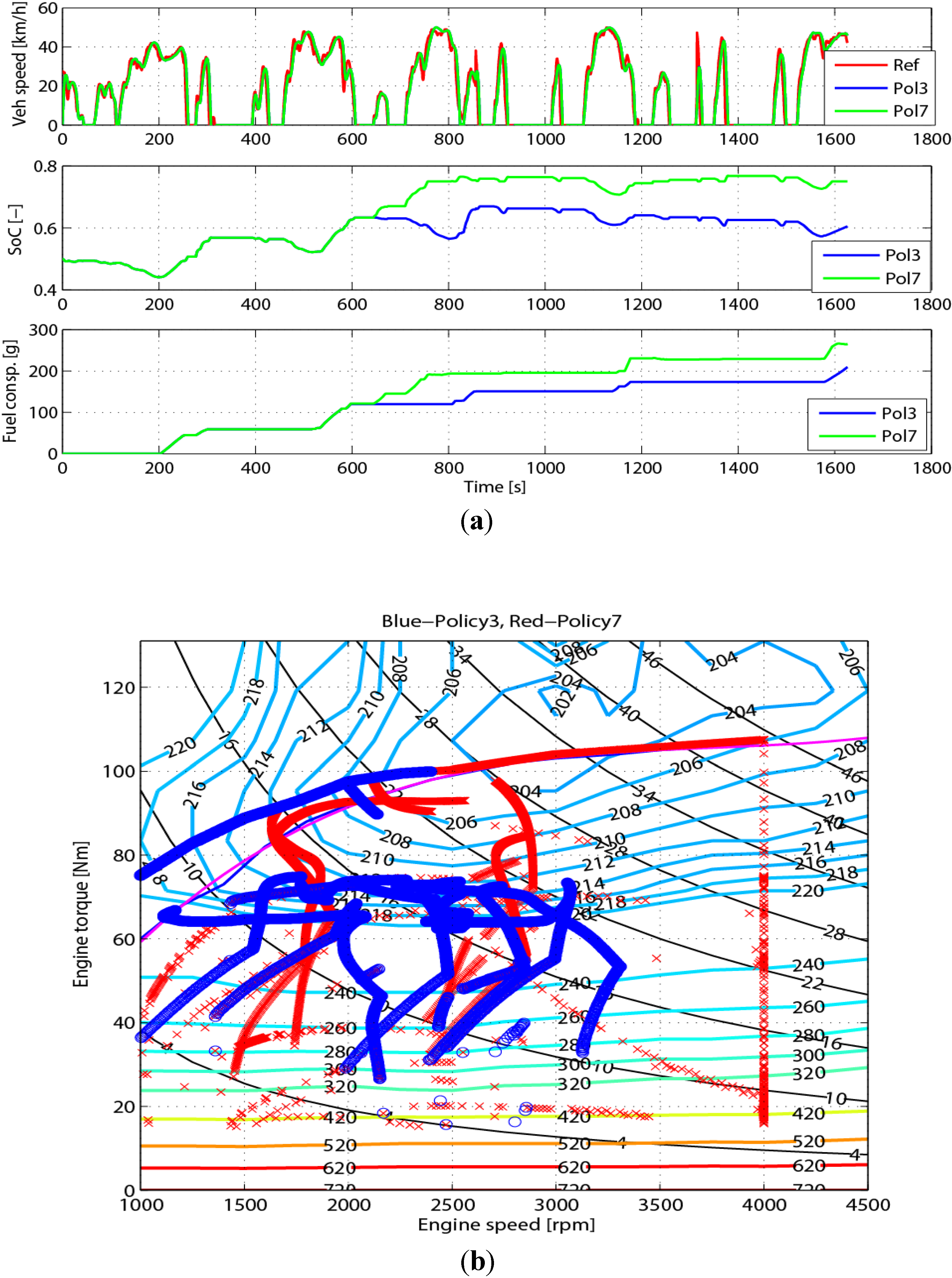
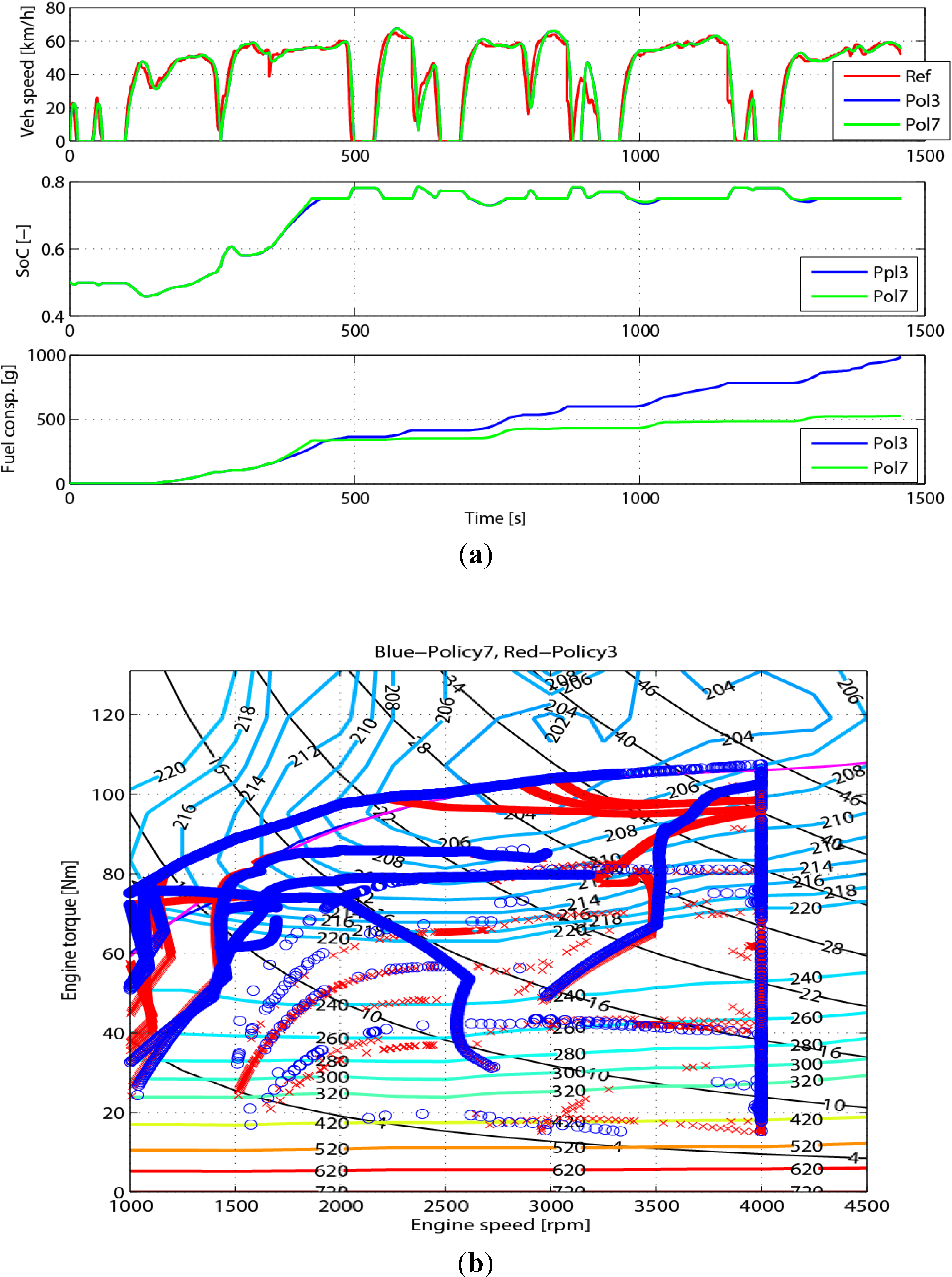
For Test case 3, the single policy-3 C₃ corresponding to the third segment and the single policy-7 C₇ corresponding to the seventh segment are chosen as examples to give the comparative validations. The comparison results of two single policies in the corresponding segment and the opposite side segment are shown in Figure 18 and Figure 19, respectively, which illustrate the effectiveness of the control policy in the corresponding segments.

Figure 18. Comparison of the policy-3 and the policy-7 in the third segment driving data. (a) Vehicle speed, SoC and fuel-electricity consumption; (b) engine operating point densities.

Figure 18. Comparison of the policy-3 and the policy-7 in the third segment driving data. (a) Vehicle speed, SoC and fuel-electricity consumption; (b) engine operating point densities.

Figure 19. Comparison of the policy-3 and the policy-7 in the seventh segment driving data. (a) Vehicle speed, SoC and fuel-electricity consumption; (b) engine operating point densities.

Figure 19. Comparison of the policy-3 and the policy-7 in the seventh segment driving data. (a) Vehicle speed, SoC and fuel-electricity consumption; (b) engine operating point densities.

5. Conclusions

Utilizing traffic information instead of some reference driving cycles, we present a power splitting strategy to minimize fuel-electricity consumptions for commuter hybrid electric vehicles. The traffic information in a certain segment of the route is modeled as a stationary Markov chain by extracting the statistical characteristic of driving speed profiles. Consequently, the power split problem is converted into a discrete stochastic optimization problem, in which considering the compromises between the benefit of computing requirement and the expense of reduced performance, only SoC is regarded as system state, and the averaged speed in term of distance is interpreted as stochastic disturbance.

It is noted that the stochastic optimization problem is formulated in terms of segments with similar statistical characteristics. Therefore, by a modified policy iteration algorithm of the SDP, the optimal solution is the control policy in a certain segment. The control policy in the route should consist of the corresponding control policy applicable to each segment of the whole route. Furthermore, the designed control strategy applies to the basic operation modes of the HEV powertrain. Besides that, the torque-split controller in the real-time implementation of energy management includes some logical strategies in terms of the limitations for thermal and/or mechanical conditions as well as a whole operation range of boundary conditions.

For the effectiveness validation, three test cases are done in a HEV simulator on the Matlab/Simulink platform by utilizing a 15 day sample of driving speed profiles. In general, the simulation results show the better performance of the proposed strategy on fuel economy, charge sustenance, and drivability, even though there are exceptions in individual driving speed profiles.

On the other hand, since there is no doubt that the control policy of the stochastic optimization problem is dependent on the adequate statistical analysis, admittedly, it is necessary to probe further into the issue whether the collected data adequate enough for statistical analysis.