Experimental Analysis of the Input Variables’ Relevance to Forecast Next Day’s Aggregated Electric Demand Using Neural Networks


Abstract
:1. Introduction
2. Data, Tools and Methodologies to Be Used in the Study
2.1. Dataset Employed
2.2. Methodology
2.2.1. Analysis of the Variables of Interest
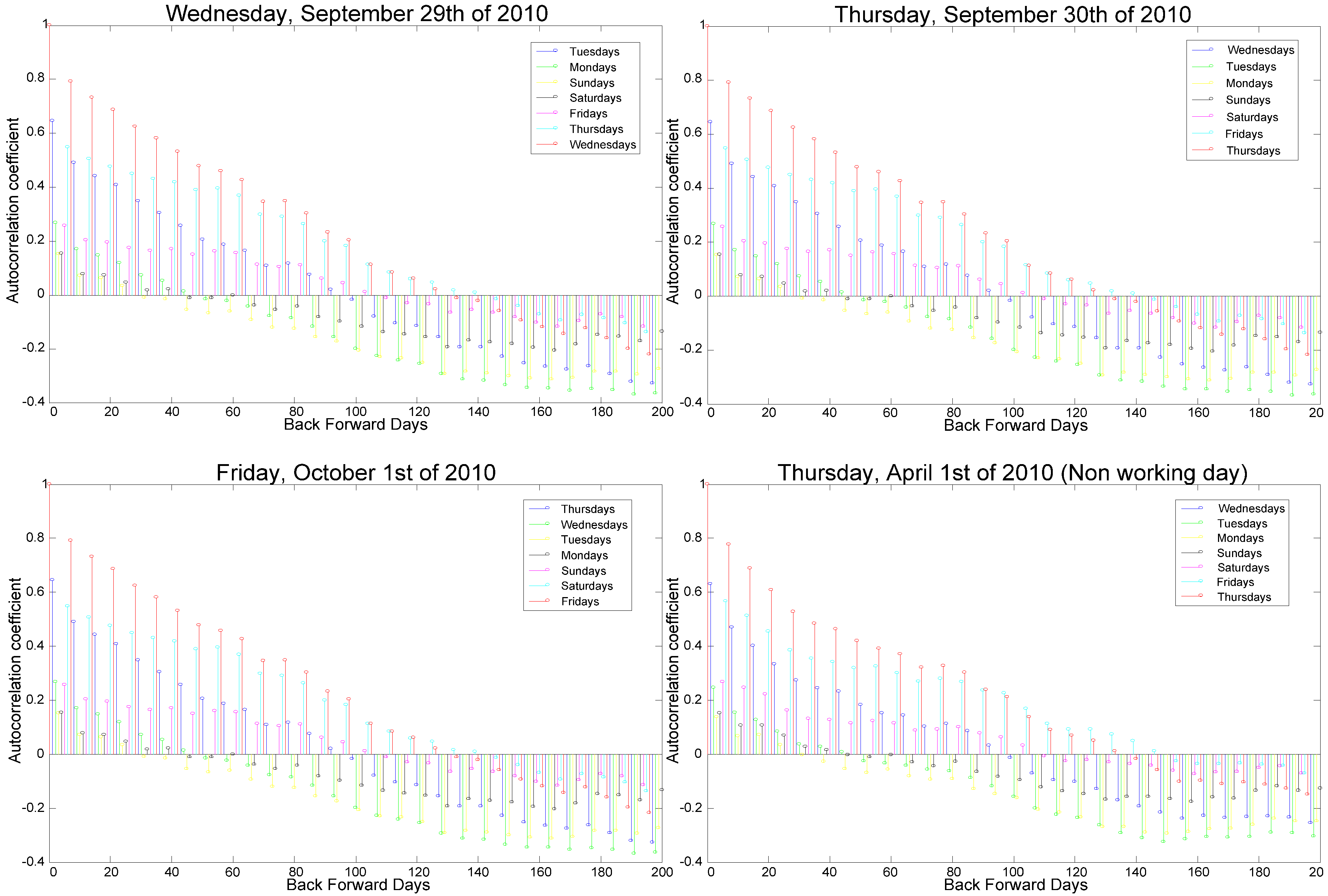
- Past aggregated load: an autocorrelation analysis will be carried out to detect the influence of the previous days’ aggregated load on the next day’s demand.
- Climate variables: those variables that have a most significant influence on the aggregated load will be detected.
- r = +1: perfect positive linear correlation.
- 0.0 < |r| < 0.09: no correlation.
- 0.1 < |r| < 0.25: small linear correlation.
- 0.26 < |r| < 0.55: medium linear correlation.
- 0.56 < |r| < 1: strong linear correlation.
- r = 0: both variables are not linearly related.
- −1 < r < 0: negative linear correlation.
- r = −1: perfect negative linear correlation.
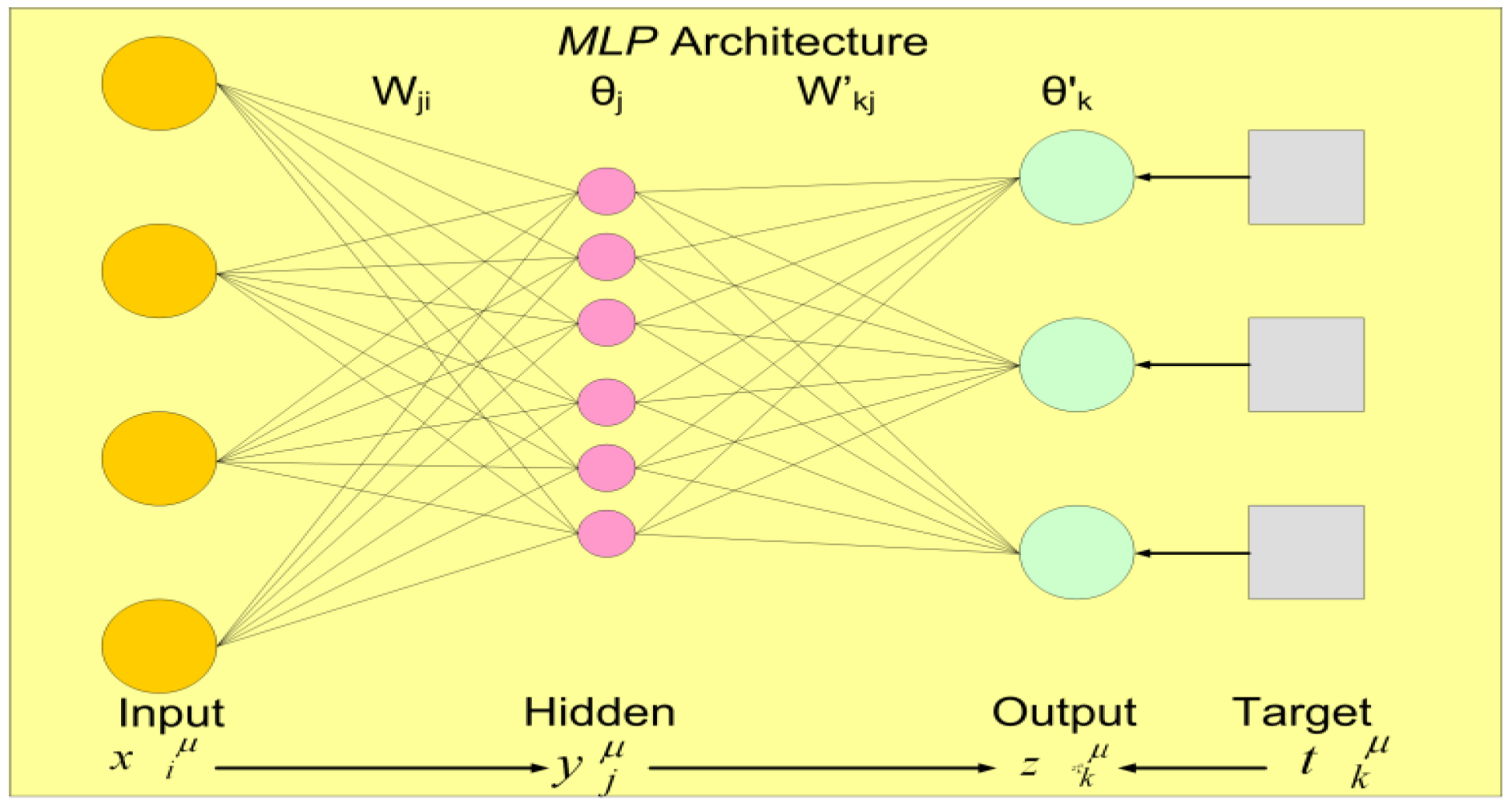
2.2.2. Forecasting Models Based on ANNs
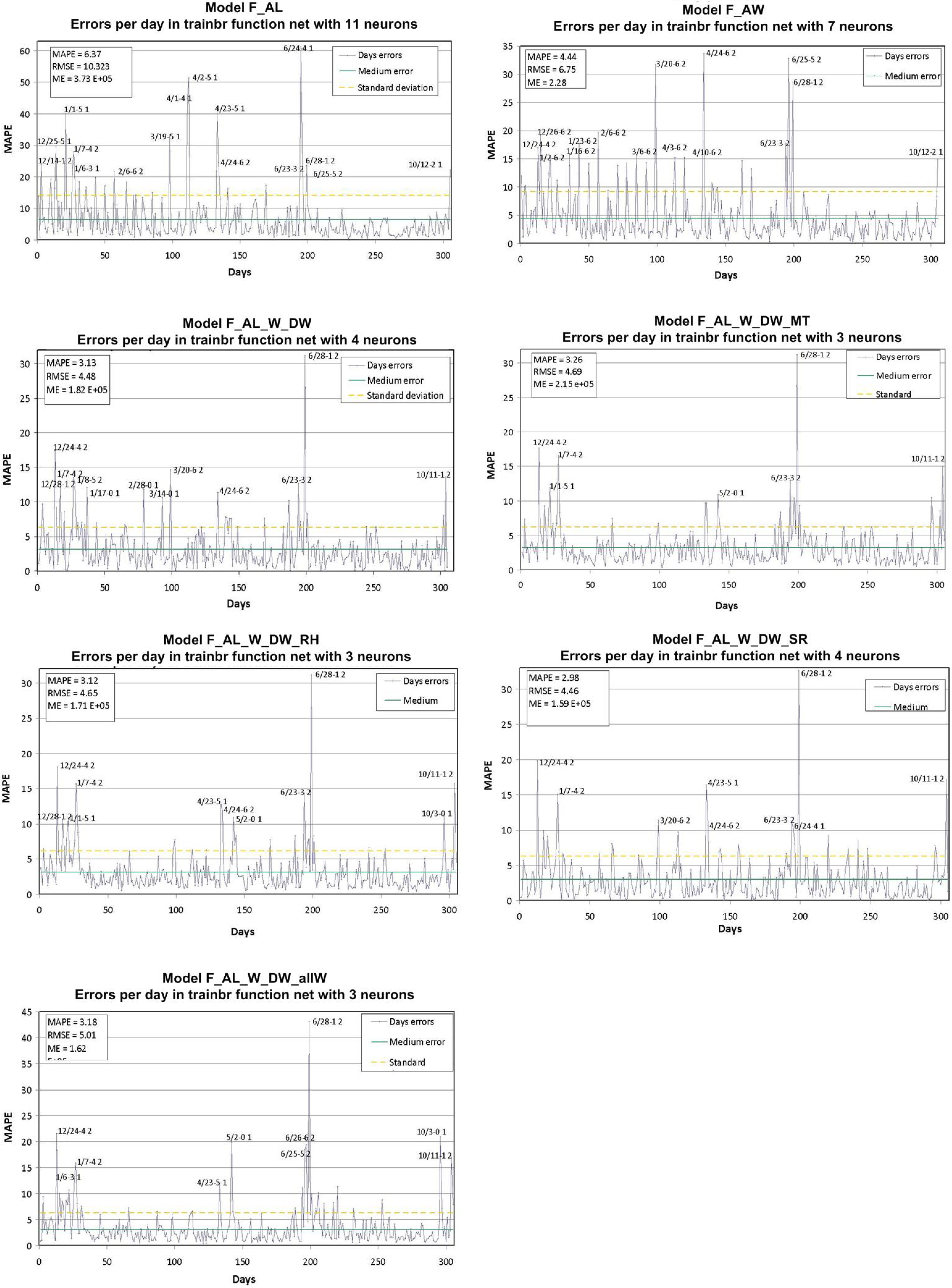
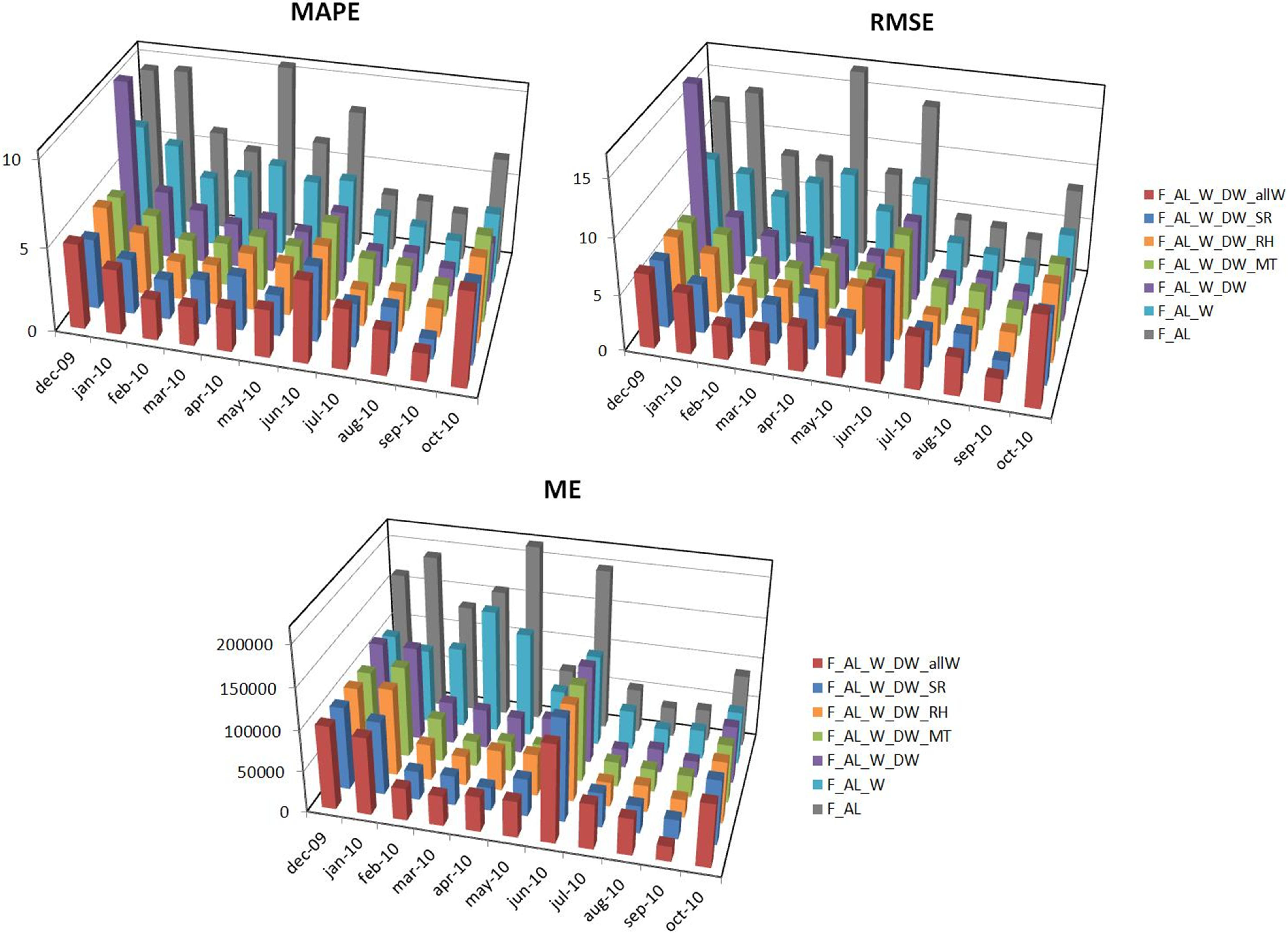
- Mean Absolute Percentage Error (MAPE): this is the most widely used measure by the industry, and thus allows comparing the results with previous studies. MAPE error is defined as:where is the aggregated load corresponding to day i; is the forecast aggregated load for day i; and n is the size of the sample.
- Root Mean Square Error (RMSE): MAPE error lacks sensitivity for errors which are more than two standard deviations away from the mean. However, this kind of error, though uncommon, is of great importance for utilities. Obviously, the weight of big deviations is greater for a squared function than for the absolute value function, and therefore the former has been selected. RMSE error is defined as:
- Maximum Error (ME): this measure complements the previous two and evaluates the maximum difference between the forecasts and the real values. A single but very big deviation could have dramatic consequences for a production system. ME error is defined as:
3. Analysis of the Relevant Variables to Forecast the Aggregated Load
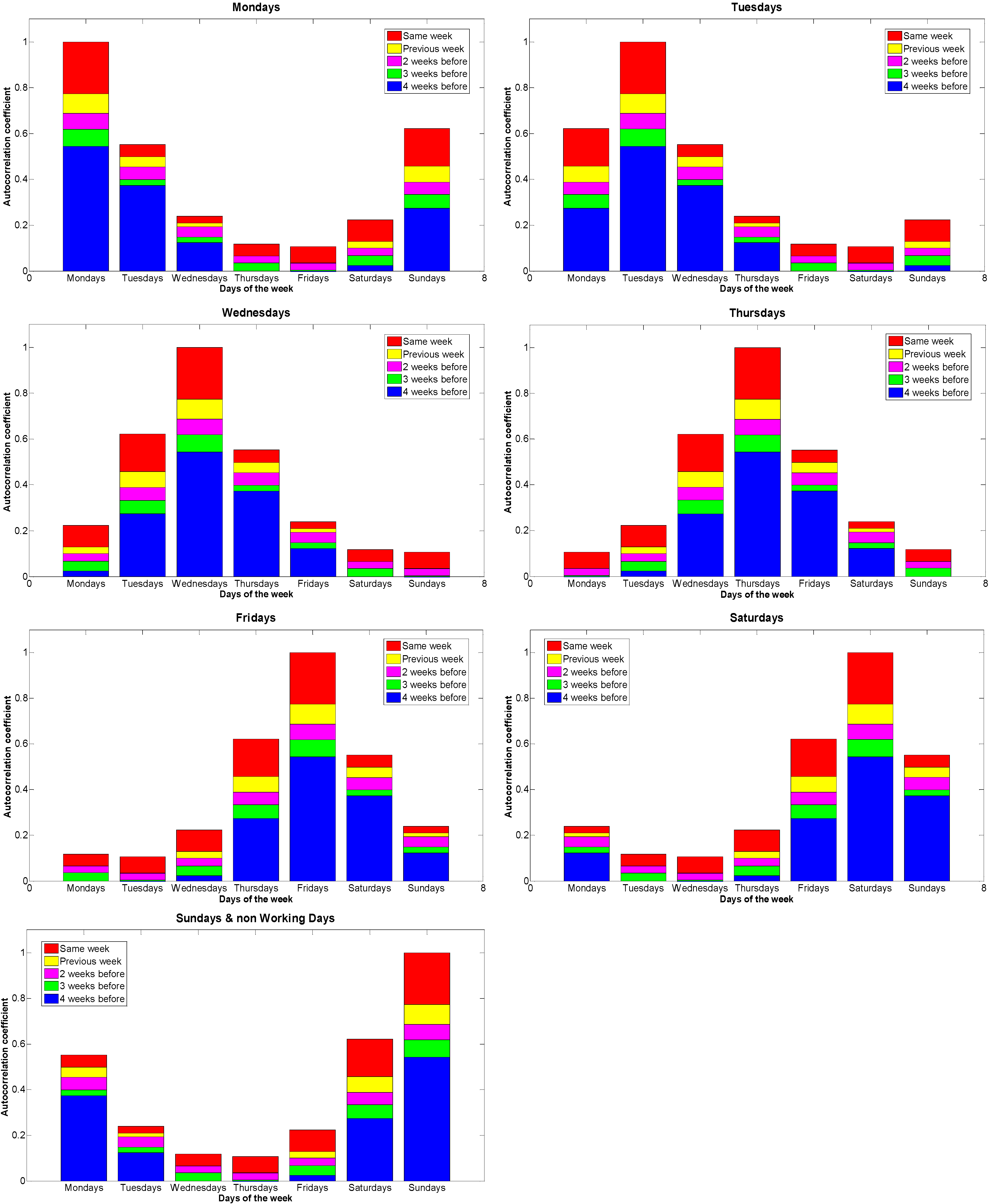
3.1. Autocorrelation of Aggregated Load
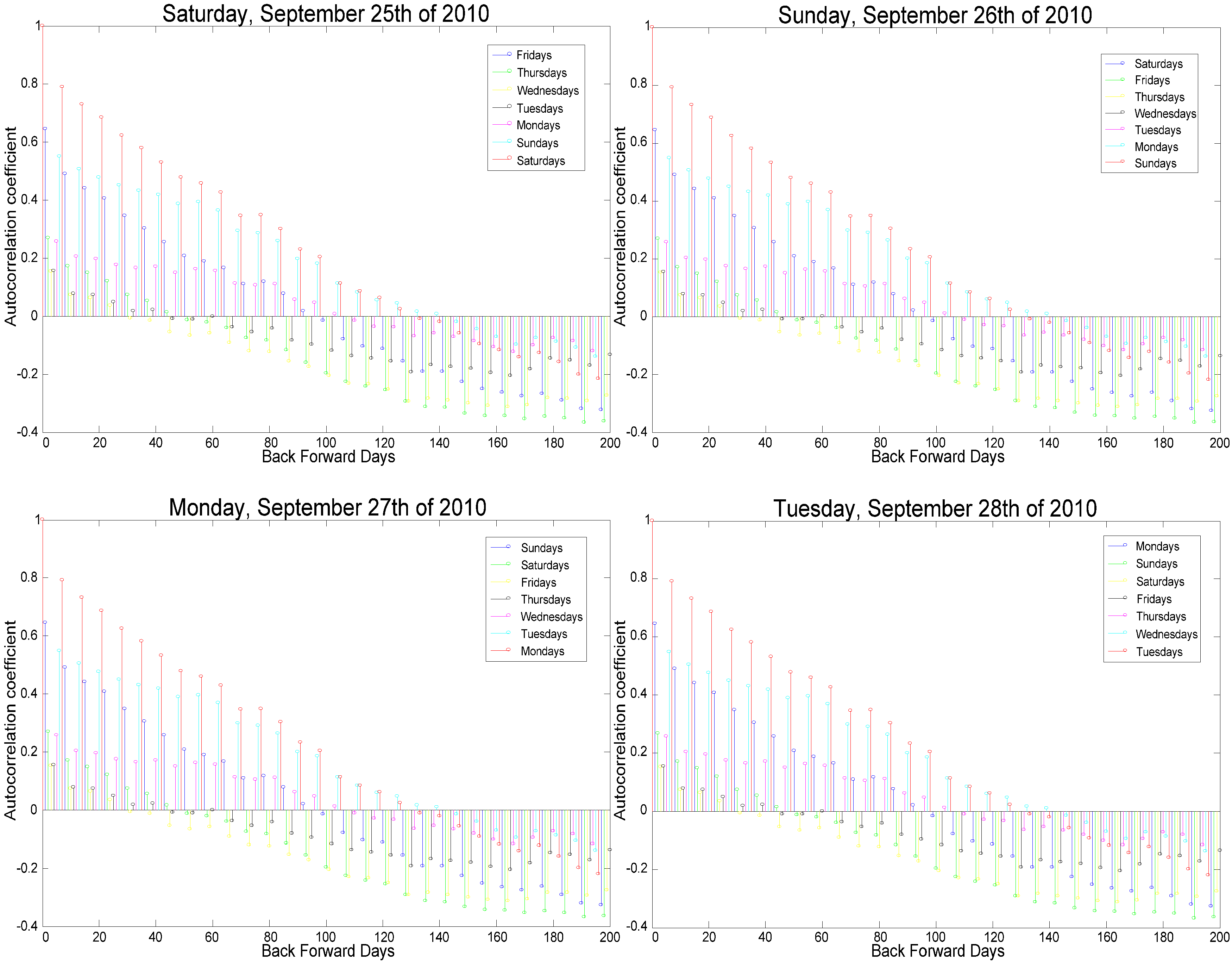

- Working days correlate with the day coming immediately before them and with the same day of the week for the previous three weeks.
- Similarly, non-working days correlate with the day coming immediately before them and with the same day of the week for the previous two weeks.

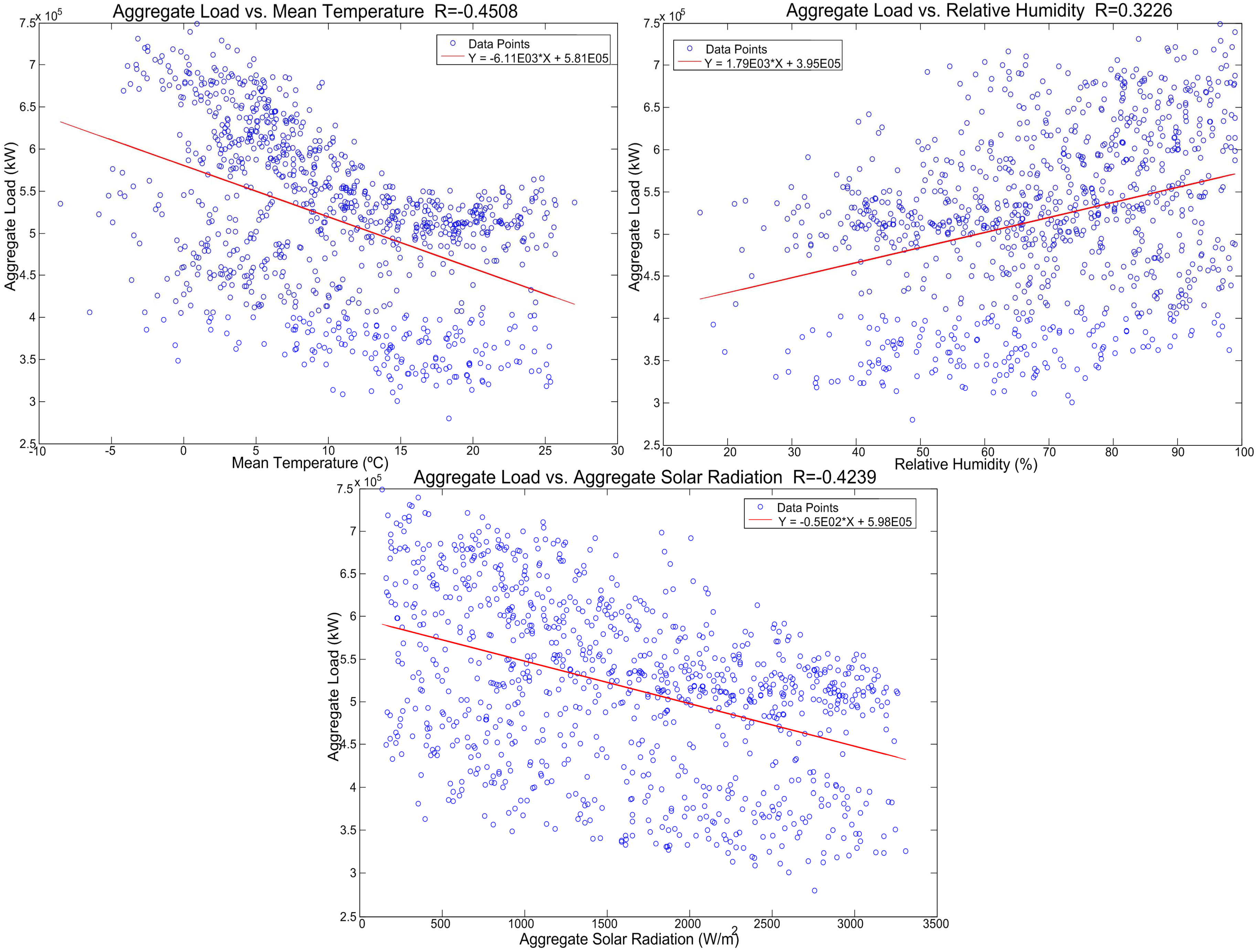
3.2. Climate Variables

| All days | AL | MT | MRH | ASR | MWD | MWS | MP |
|---|---|---|---|---|---|---|---|
| AL | 1.00000 | −0.4508 | 0.3226 | −0.4239 | 0.25437 | 0.20064 | 0.02355 |
| MT | −0.4508 | 1.00000 | −0.61656 | −0.09186 | −0.19514 | −0.23928 | 0.05872 |
| MRH | 0.32157 | −0.61656 | 1.00000 | 0.27902 | 0.08449 | 0.24059 | −0.06951 |
| ASR | −0.4239 | −0.09186 | 0.27902 | 1.00000 | 0.16316 | 0.01912 | 0.00309 |
| MWD | 0.25437 | −0.19514 | 0.08449 | 0.16316 | 1.00000 | 0.32152 | −0.07974 |
| MWS | 0.20064 | −0.23928 | 0.24059 | 0.01912 | 0.32152 | 1.00000 | −0.08816 |
| MP | 0.02355 | 0.05872 | −0.06951 | 0.00309 | −0.07974 | −0.08816 | 1.00000 |
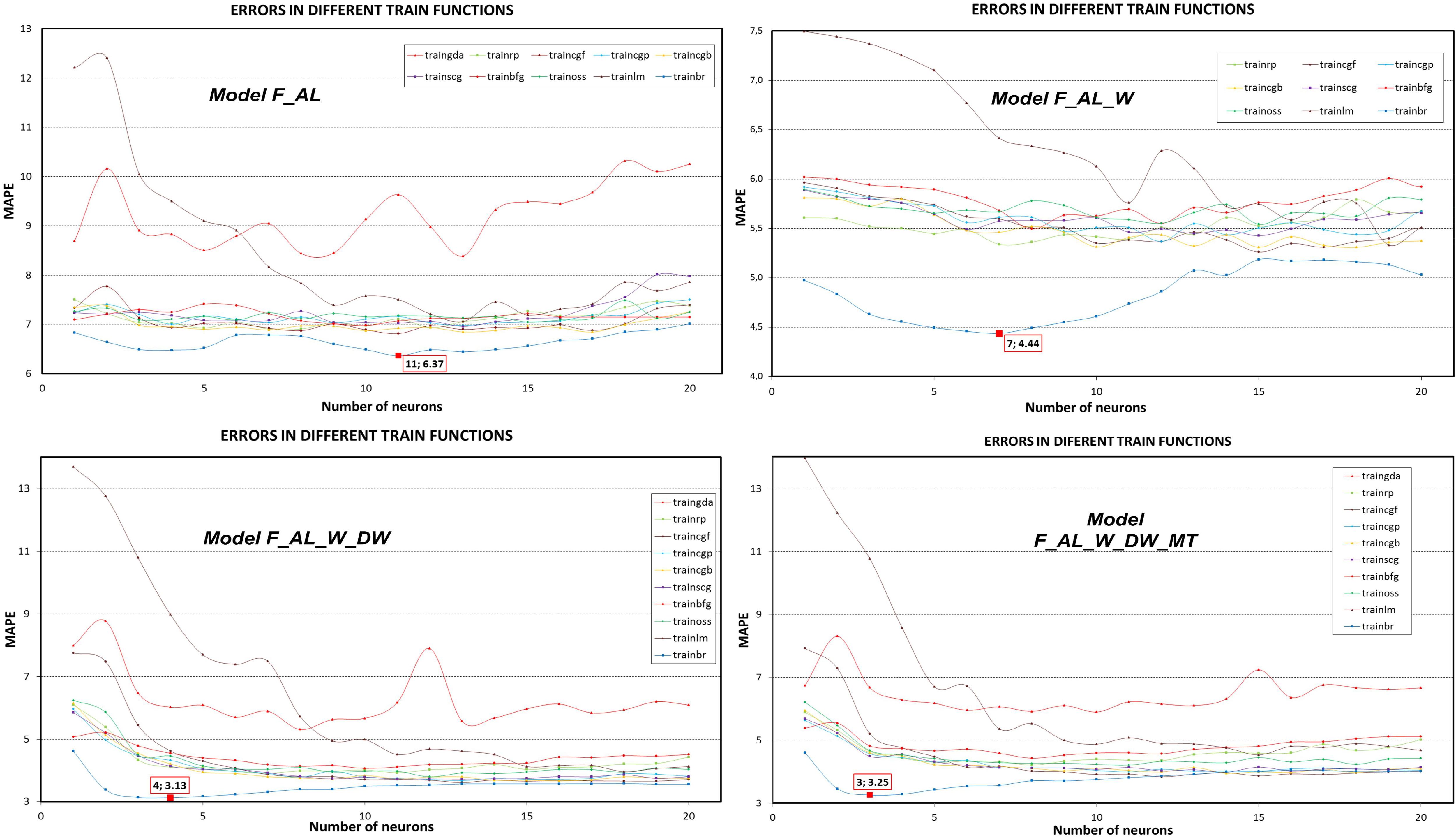
4. Models Proposed to Forecast the Aggregated Load

- Forecast with Aggregated Load (F_AL): as shown in Section 3.1, aggregated load is closely related to the previous day’s aggregated load, as well as to aggregated loads corresponding to the same day of the week for the previous three weeks, regardless of whether this is a working day or not, and this holds for all days of the week. With this in mind, in the F_AL model the chosen inputs are the aggregated load of the previous day, and the same days of the week, of the previous three weeks. This makes 4 inputs and 1 target.
- Forecast with Aggregated Load and Type of Day [working/non-working](F_AL_W): five new variables are added to the F_AL, indicating whether each of the days is a working day or not. They refer to the past days and the day for which the forecast is made. This makes nine inputs and one target.
- Forecast with Aggregated Load, Type of Day (working/non-working) and Day of the Week (F_AL_WD): 10 new variables are added to the F_AL_W, indicating the day of the week (Sunday = 0; Monday = 1; Friday = 5; Saturday = 6) in the sine and cosine forms. These refer to the past days and the day to be forecast. This makes 19 inputs and one target. As mentioned, for circular variables (days of the week, etc.), the use of two inputs for each variable (in its sine and cosine forms) has been shown to improve performance, since values are uniformly distributed between 0 and 2π, allowing the network to perceive periodic behavior more efficiently and reducing training time, as shown in Ramezani et al. [34] and in Razavi and Tolson [35].
- Forecast with Aggregated Load, Type of Day (working/non-working), Day of the Week and Mean Temperature (F_AL_W_DW_MT): In this model, five new variables are added to the F_AL_W_DW, representing the mean temperature of the past days and the day for which the forecast is made. This makes 24 inputs and one target.
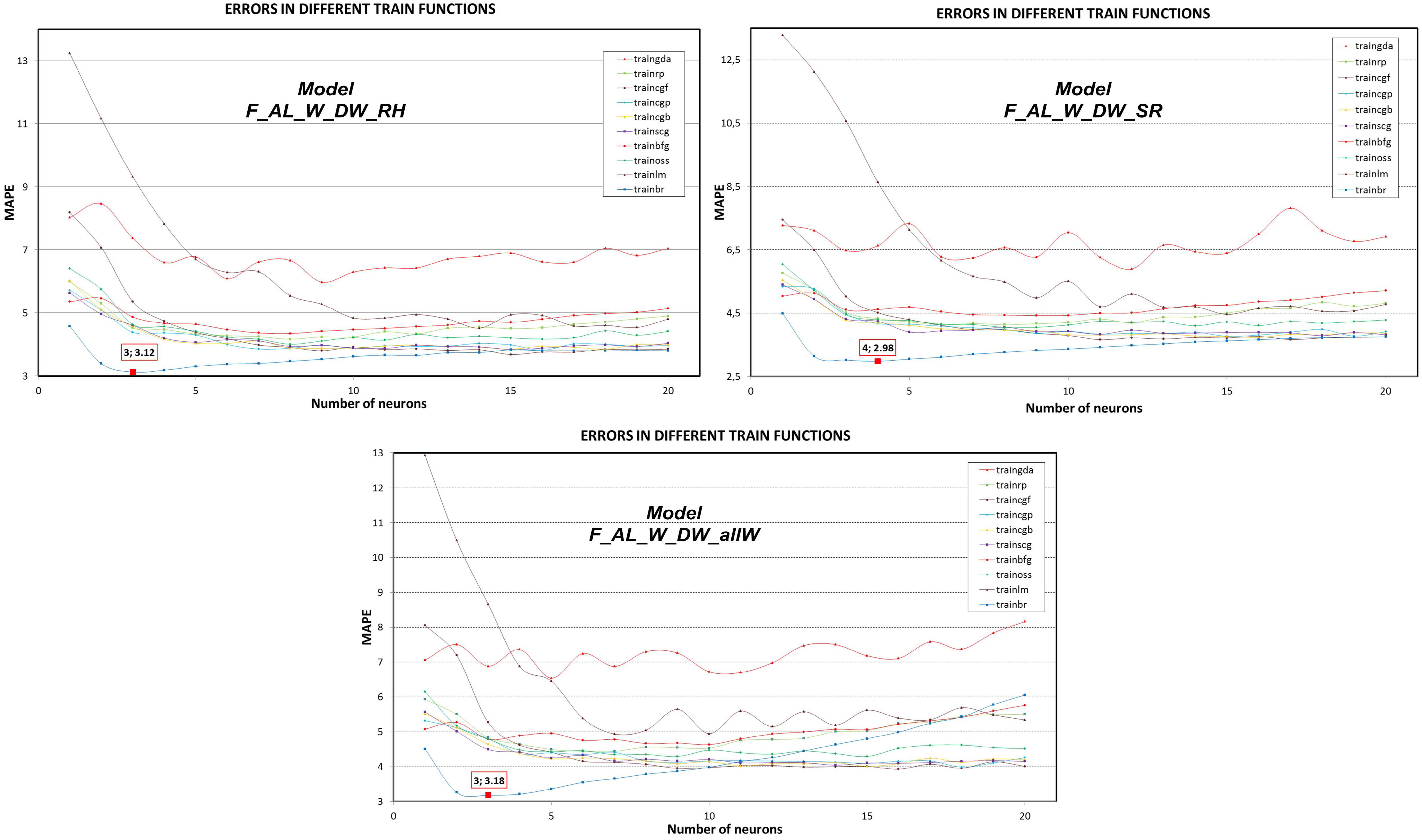
- Forecast with Aggregated Load, Type of Day (working/non-working), Day of the Week and Relative Humidity (F_AL_W_DW_RH): In this model, five new variables are added to the F_AL_W_DW, representing the relative humidity of the past days and the day for which the forecast is made. This makes 24 inputs and one target.
- Forecast with Aggregated Load, Type of Day (working/non-working), Day of the Week and Solar Radiation (F_AL_W_DW_SR): In this model, five new variables are added to the F_AL_W_DW, representing the solar radiation of the past days and the day for which the forecast is made. This makes 24 inputs and one target.
- Forecast with Aggregated Load, Type of Day (working/non-working), Day of the Week (F_AL_W) and all Weather (F_AL_W_DW_allW): In this model, 15 new variables are added to the F_AL_W_DW, representing the mean temperature, relative humidity and solar radiation of the past days and the day for which the forecast is made. This makes 34 inputs and one target.
5. Results
| traingd | traingdm | traingda | traingdx | trainrp | traincgf | traincgp | |||||||||||||||
| (1) | (2) | (3) | (1) | (2) | (3) | (1) | (2) | (3) | (1) | (2) | (3) | (1) | (2) | (3) | (1) | (2) | (3) | (1) | (2) | (3) | |
| F_AL | 1 | 27.84 | 9.13 | 1 | 27.99 | 8.70 | 13 | 8.39 | 0.96 | 1 | 27.07 | 8.67 | 7 | 6.90 | 0.46 | 11 | 6.81 | 0.37 | 13 | 6.98 | 0.53 |
| F_AL_W | 5 | 40.87 | 18.85 | 5 | 39.26 | 18.59 | 6 | 7.09 | 1.64 | 5 | 42.20 | 19.12 | 7 | 5.34 | 0.42 | 15 | 5.26 | 0.42 | 12 | 5.37 | 0.51 |
| F_AL_W_DW | 1 | 30.92 | 9.04 | 1 | 28.47 | 8.67 | 8 | 5.31 | 1.09 | 1 | 29.70 | 10.38 | 7 | 3.90 | 0.44 | 13 | 3.61 | 0.36 | 13 | 3.67 | 0.51 |
| F_AL_W_DW_MT | 1 | 29.90 | 8.99 | 1 | 28.93 | 10.08 | 10 | 5.89 | 1.05 | 1 | 30.39 | 8.82 | 8 | 4.21 | 0.47 | 12 | 3.83 | 0.39 | 11 | 3.99 | 0.51 |
| F_AL_W_DW_RH | 1 | 27.67 | 8.01 | 1 | 29.52 | 9.64 | 9 | 5.98 | 1.15 | 1 | 29.35 | 9.19 | 8 | 4.16 | 0.54 | 15 | 3.68 | 0.42 | 16 | 3.82 | 0.41 |
| F_AL_W_DW_SR | 1 | 28.96 | 9.89 | 1 | 29.01 | 9.24 | 12 | 5.89 | 1.21 | 1 | 29.80 | 8.44 | 8 | 4.13 | 0.60 | 17 | 3.66 | 0.48 | 15 | 3.77 | 0.40 |
| F_AL_W_DW_allW | 1 | 28.14 | 9.43 | 1 | 29.01 | 9.31 | 5 | 6.54 | 1.68 | 1 | 28.42 | 9.00 | 7 | 4.44 | 0.56 | 16 | 3.93 | 0.49 | 18 | 3.99 | 0.46 |
| traincgb | trainscg | trainbfg | trainoss | trainlm | trainbr | ||||||||||||||||
| (1) | (2) | (3) | (1) | (2) | (3) | (1) | (2) | (3) | (1) | (2) | (3) | (1) | (2) | (3) | (1) | (2) | (3) | ||||
| F_AL | 13 | 6.85 | 0.36 | 13 | 6.96 | 0.43 | 10 | 6.98 | 0.37 | 15 | 7.04 | 0.45 | 13 | 7.06 | 1.36 | 11 | 6.37 | 0.22 | |||
| F_AL_W | 18 | 5.31 | 0.51 | 15 | 5.43 | 0.52 | 8 | 5.49 | 0.35 | 15 | 5.54 | 0.51 | 19 | 5.33 | 0.84 | 7 | 4.44 | 0.15 | |||
| F_AL_W_DW | 16 | 3.66 | 0.43 | 13 | 3.72 | 0.57 | 10 | 4.06 | 0.34 | 12 | 3.79 | 0.46 | 18 | 3.96 | 0.85 | 4 | 3.13 | 0.17 | |||
| F_AL_W_DW_MT | 14 | 3.95 | 0.48 | 14 | 3.96 | 0.56 | 8 | 4.42 | 0.49 | 11 | 4.21 | 0.68 | 15 | 4.53 | 0.79 | 3 | 3.26 | 0.18 | |||
| F_AL_W_DW_RH | 15 | 3.85 | 0.41 | 15 | 3.84 | 0.51 | 8 | 4.35 | 0.45 | 8 | 4.01 | 0.64 | 14 | 4.52 | 1.45 | 3 | 3.12 | 0.17 | |||
| F_AL_W_DW_SR | 16 | 3.73 | 0.47 | 18 | 3.79 | 0.58 | 9 | 4.43 | 0.64 | 8 | 4.05 | 0.62 | 15 | 4.46 | 1.64 | 4 | 2.98 | 0.15 | |||
| F_AL_W_DW_allW | 15 | 4.02 | 0.40 | 14 | 4.05 | 0.48 | 10 | 4.64 | 0.51 | 9 | 4.29 | 0.64 | 17 | 4.94 | 1.29 | 3 | 3.18 | 0.19 | |||
- Non-working days that fall on weekdays, as well as some days that immediately follow them. Since no additional information is available for the different patterns, the network did not take into account whether the day was a working day. The period between 23 June and 28 June, which corresponds to the local festivals. Except for Thursday 24, and Sunday 27, which are non-working days, the rest of the days within the period are working days, but in practice they are similar to non-working days. As previously, this information is not available for the network.
- A high number of Saturdays show an error between 15% and 25%. This can be explained considering that Saturdays are working days (the network forecasts a high aggregated load value), but in fact aggregated load is lower than on the Monday-Friday period. From the previous analysis, the need for the model to know whether the days are working days becomes clear. Therefore, the F_AL_W model uses this variable as an input, for the past days and the forecast day. As it can be observed in Figure 6, the model still fails during the local festivals’ week, as well as on Saturdays. However, the error for non-working days is lower than the mean in all cases, i.e., adding the new variable (working/non-working) as an input improves the forecast.


6. Conclusions and Future Work
Acknowledgements
Conflict of Interest
References
- Zhang, Q.; Lai, K.K.; Niu, D.; Wang, Q.; Zhang, X. A fuzzy group forecasting model based on least squares support vector machine (LS-SVM) for short-term wind power. Energies 2012, 5, 3329–3346. [Google Scholar] [CrossRef]
- Hsu, C.-C.; Chen, C.-Y. Regional load forecasting in Taiwan—Applications of artificial neural networks. Energy Convers. Manag. 2003, 44, 1941–1949. [Google Scholar] [CrossRef]
- Pilo, F.; Pisano, G.; Soma, G.G. Neural Implementation of Microgrid Central Controllers. In Proceedings of the 5th IEEE International Conference on Industrial Informatics, Vienna, Austria, 23–27 June 2007; pp. 1177–1182.
- Carpaneto, E.; Chicco, G. Probabilistic characterisation of the aggregated residencial load patterns. IET Gener. Transm. Distrib. 2008, 2, 373–382. [Google Scholar] [CrossRef]
- Fan, S.; Methaprayoon, K.; Lee, W.-L. Multiregion load forecasting for system with large geographical area. IEEE Trans. Ind. Appl. 2009, 45, 1452–1459. [Google Scholar] [CrossRef]
- Pudjianto, D.; Ramsay, C.; Strbac, G. Virtual power plant and system integration of distributed energy resources. IET Renew. Power Gener. 2007, 1, 10–16. [Google Scholar] [CrossRef]
- Ruiz, N.; Cobelo, I.; Oyarzabal, J. A direct load control model for virtual power plant management. IEEE Trans. Power Syst. 2009, 24, 959–966. [Google Scholar] [CrossRef]
- Hernández, L.; Baladrón, C.; Aguiar, J.M.; Carro, B.; Sánchez-Esguevillas, A.; Lloret, J.; Chinarro, D.; Gómez-Sanz, J.J.; Cook, D. A multi-agent system architecture for smart grid management and forecasting of energy demand in virtual power plants. IEEE Commun. Mag. 2013, 51, 106–113. [Google Scholar] [CrossRef]
- Paoletti, S.; Casini, M.; Giannitrapani, A.; Facchini, A.; Garulli, A.; Vicino, A. Load Forecasting for Active Distribution Networks. In Proceedings of the 2nd IEEE PES International Conference and Exhibition on Innovative Smart Grid Technologies (ISGT Europe), Manchester, UK, 5–7 December 2011.
- Mousavi, S.M.; Abyaneh, H.A. Effect of load models on probabilistic characterization of aggregated load patterns. IEEE Trans. Power Syst. 2011, 26, 811–819. [Google Scholar] [CrossRef]
- Ipakchi, A.; Alboyeh, F. Grid of the future—Are we ready to transition to a smart grid? IEEE Power Energy Mag. 2009, 7, 52–62. [Google Scholar] [CrossRef]
- Naphade, M.; Banavar, G.; Harrison, C.; Paraszczak, J.; Morris, R. Smarter cities and their innovation challenges. Computer 2011, 44, 32–39. [Google Scholar] [CrossRef]
- Hernández, L.; Baladrón, C.; Aguiar, J.M.; Calavia, L.; Carro, B.; Sánchez-Esguevillas, A.; Chinarro, D.; Gómez, J.; Cook, D. A Study of the relationship between weather variables and electric power demand inside a smart grid/smart world framework. Sensors 2012, 12, 11571–11591. [Google Scholar] [CrossRef]
- Hernandez, L.; Baladrón, C.; Aguiar, J.M.; Carro, B.; Sanchez-Esguevillas, A.J.; Lloret, J. Short-term load forecasting for microgrids based on artificial neural networks. Energies 2013, 6, 1385–1408. [Google Scholar] [CrossRef]
- Pérez, E.; Beltrán, H.; Aparicio, N.; Rodríguez, P. Predictive power control for PV plants with energy storage. IEEE Trans. Sustain. Energy 2013, 4, 482–490. [Google Scholar] [CrossRef]
- Ogliary, E.; Grimaccia, F.; Leva, S.; Musseta, M. Hybrid predictive models for accurate forecasting in PV systems. Energies 2013, 6, 1918–1929. [Google Scholar] [CrossRef] [Green Version]
- Hippert, H.S.; Pedreira, C.E.; Souza, R.C. Neural networks for short-term load forecasting: A review and evaluation. IEEE Trans. Neural Netw. 2001, 16, 44–45. [Google Scholar]
- Douglas, A.P.; Breiphol, A.M.; Lee, F.N.; Adapa, R. The impacts of temperature forecast uncertainty on Bayesian load forecasting. IEEE Trans. Power Syst. 1998, 13, 1507–1513. [Google Scholar] [CrossRef]
- Sadownik, R.; Barbosa, E.P. Short-term forecasting of industrial electricity consumption in Brazil. J. Forecast 1999, 18, 215–224. [Google Scholar] [CrossRef]
- Huang, S.R. Short-term load forecasting using threshold autoregressive models. IEE Proc. Gener. Transmi. Distrib. 1997, 144, 477–481. [Google Scholar] [CrossRef]
- Infield, D.G.; Hill, D.C. Optimal smoothing for trend removal in short term electricity demand forecasting. IEEE Trans. Power System 1998, 13, 1115–1120. [Google Scholar] [CrossRef]
- Sargunaraj, S.; Sen Gupta, D.P.; Devi, S. Short-term load forecasting for demand side management. IEE Proc. Gener. Transm. Distrib. 1997, 144, 68–74. [Google Scholar] [CrossRef]
- Yang, H.T.; Huang, C.M. A new short-term load forecasting approach using self-organizing fuzzy ARMAX models. IEEE Trans. Power Syst. 1998, 13, 217–225. [Google Scholar] [CrossRef]
- Yang, H.T.; Huang, C.M.; Huang, C.L. Identification of ARMAX model for short term load forecasting: An evolutionary programming approach. IEEE Trans. Power Syst. 1996, 11, 403–408. [Google Scholar] [CrossRef]
- Yu, Z. A temperature match based optimization method for daily load prediction considering DLC effect. IEEE Trans. Power Syst. 1996, 11, 728–733. [Google Scholar] [CrossRef]
- Charytoniuk, W.; Chen, M.S.; Van Olinda, P. Nonparametric regression based short-term load forecasting. IEEE Trans. Power Syst. 1998, 13, 725–730. [Google Scholar] [CrossRef]
- Taylor, J.W.; Majithia, S. Using combined forecast with changing weights for electricity demand profiling. J. Oper. Res. Soc. 2000, 51, 77–82. [Google Scholar]
- Ramanathan, R.; Engle, E.; Granger, C.W.J.; Vahid-Araghi, F.; Brace, C. Short-run forecasts of electricity load and peaks. Int. J. Forecast 1997, 144, 161–174. [Google Scholar] [CrossRef]
- Rumelhart, D.; Hinton, G.; Williams, R. Learning Internal Representations by Error Propagation. In Parallel Distributed Processing: Explorations in the Microstructure of Cognition; Rumelhart, D., McClelland, J.L., Eds.; MIT Press: Cambridge, MA, USA, 1996; Volume 1, pp. 318–362. [Google Scholar]
- Broomhead, D.S.; Lowe, D. Multivariable functional interpolation and adaptive networks. Complex Syst. 1988, 2, 321–355. [Google Scholar]
- Elman, J.L. Finding structure in time. Cognit. Sci. 1990, 14, 179–211. [Google Scholar] [CrossRef]
- Elman, J.L. Distributed representations, simple recurrent networks, and grammatical structure. Mach. Learn. 1991, 7, 95–126. [Google Scholar]
- Kohonen, T. The self-organizing map. Proc. IEEE 1990, 78, 1464–1480. [Google Scholar] [CrossRef]
- Ramezani, M.; Falaghi, H.; Haghifam, M.-R. Short-Term Electric Load Forecasting Using Neural Networks. In Proceedings of the International Conference on Computers as a Tool, Belgrade, Serbia & Montenegro, 21–24 November 2005; Volume 2, pp. 1525–1528.
- Razavi, S.; Tolson, B.A. A new formulation for feedforward neural networks. IEEE Trans. Neural Netw. 2011, 22, 1588–1598. [Google Scholar] [CrossRef] [PubMed]
© 2013 by the authors; licensee MDPI, Basel, Switzerland. This article is an open access article distributed under the terms and conditions of the Creative Commons Attribution license (http://creativecommons.org/licenses/by/3.0/).
Share and Cite
Hernández, L.; Baladrón, C.; Aguiar, J.M.; Calavia, L.; Carro, B.; Sánchez-Esguevillas, A.; García, P.; Lloret, J. Experimental Analysis of the Input Variables’ Relevance to Forecast Next Day’s Aggregated Electric Demand Using Neural Networks. Energies 2013, 6, 2927-2948. https://doi.org/10.3390/en6062927
Hernández L, Baladrón C, Aguiar JM, Calavia L, Carro B, Sánchez-Esguevillas A, García P, Lloret J. Experimental Analysis of the Input Variables’ Relevance to Forecast Next Day’s Aggregated Electric Demand Using Neural Networks. Energies. 2013; 6(6):2927-2948. https://doi.org/10.3390/en6062927
Chicago/Turabian StyleHernández, Luis, Carlos Baladrón, Javier M. Aguiar, Lorena Calavia, Belén Carro, Antonio Sánchez-Esguevillas, Pablo García, and Jaime Lloret. 2013. "Experimental Analysis of the Input Variables’ Relevance to Forecast Next Day’s Aggregated Electric Demand Using Neural Networks" Energies 6, no. 6: 2927-2948. https://doi.org/10.3390/en6062927