Numerical Model of a Variable-Combined-Cycle Engine for Dual Subsonic and Supersonic Cruise

Abstract
:
1. Introduction


| Mach Range | Regime | Mode | Bypass Burner | Bypass Nozzle |
|---|---|---|---|---|
| 0.0–0.9 | Subsonic Acceleration | Turbofan | On | Open |
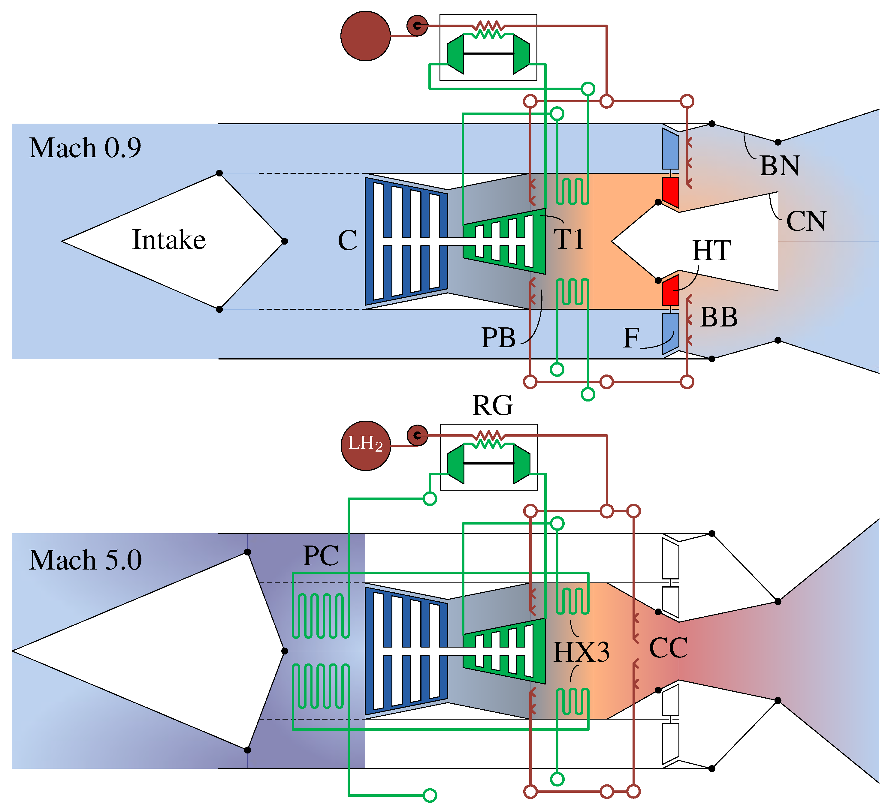
| 0.9 | Subsonic Cruise | Turbofan | Off | Fully Open |
| 0.9–2.5 | Supersonic Acceleration | Turbofan | On | Open |
| 2.5–5.0 | Supersonic Acceleration | Ramjet + ATR | On | Open |
| 5.0 | Supersonic Cruise | ATR | Off | Closed |
2. Numerical Model

2.1. Intake
2.2. Combustion Chambers and Nozzle
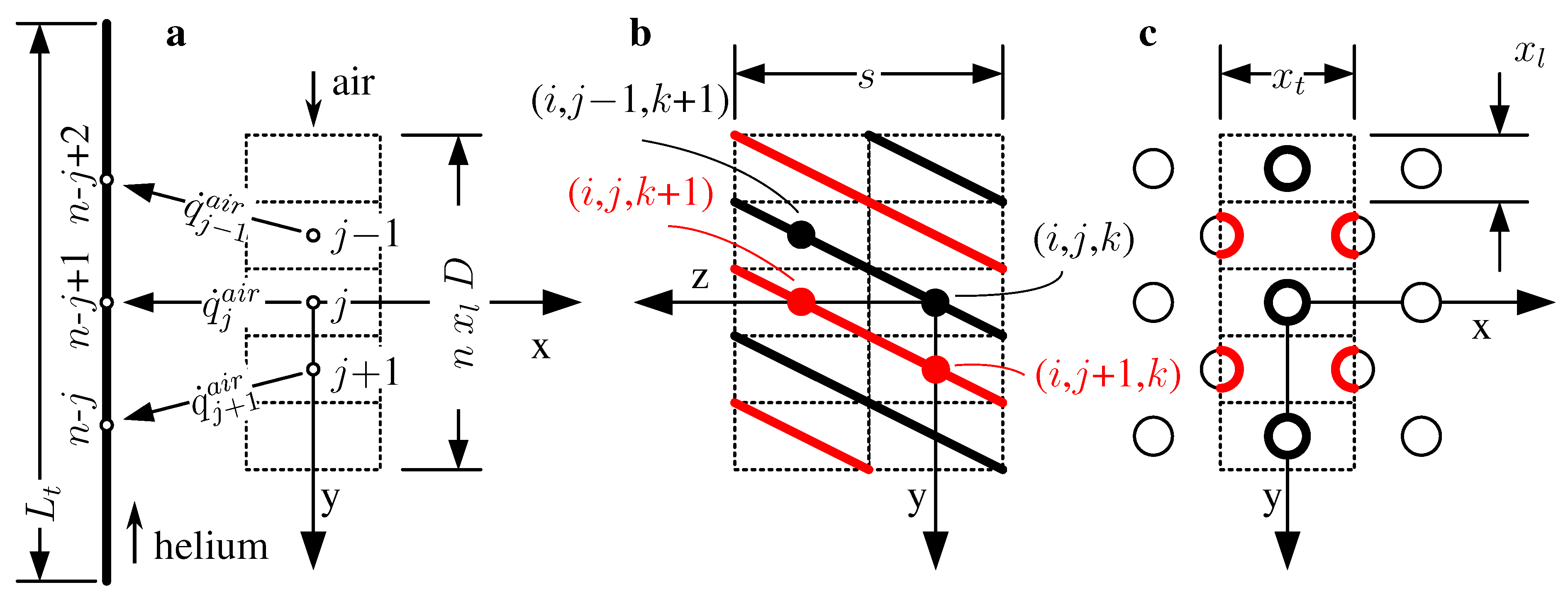
2.3. Heat Exchangers
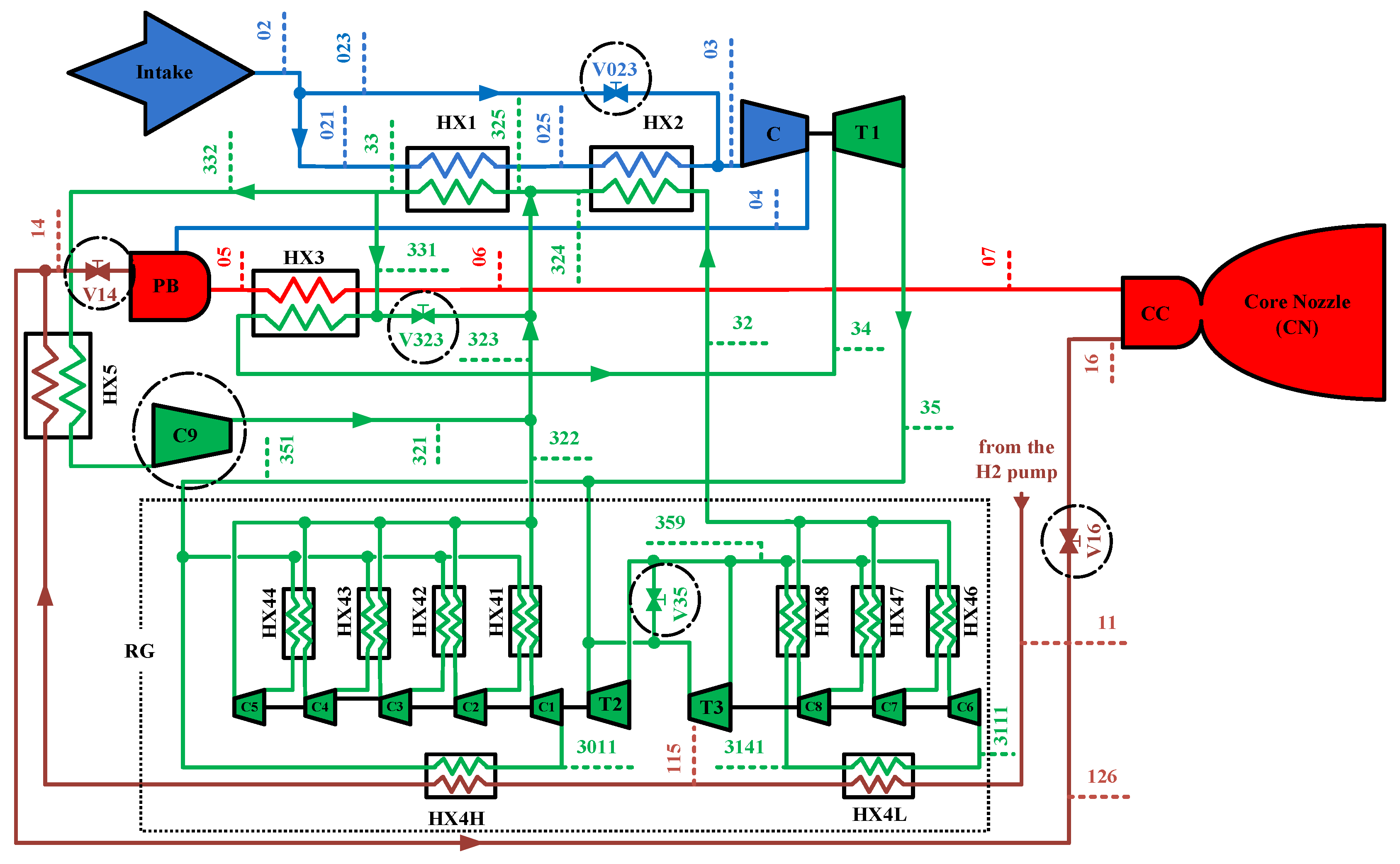
2.3.1. Precooler


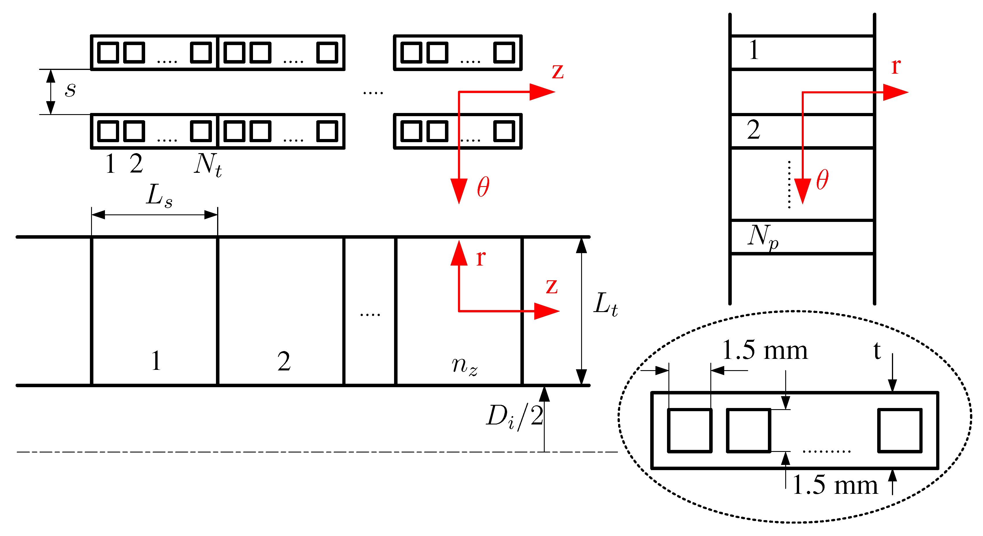
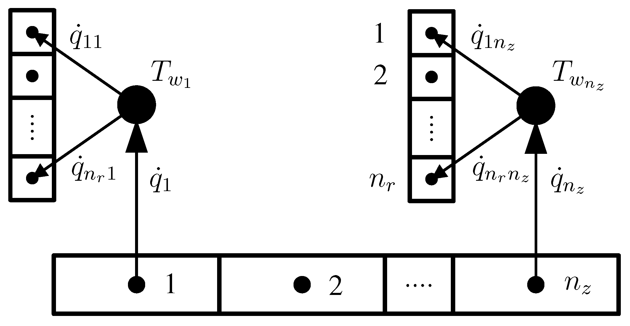
2.3.2. Reheater


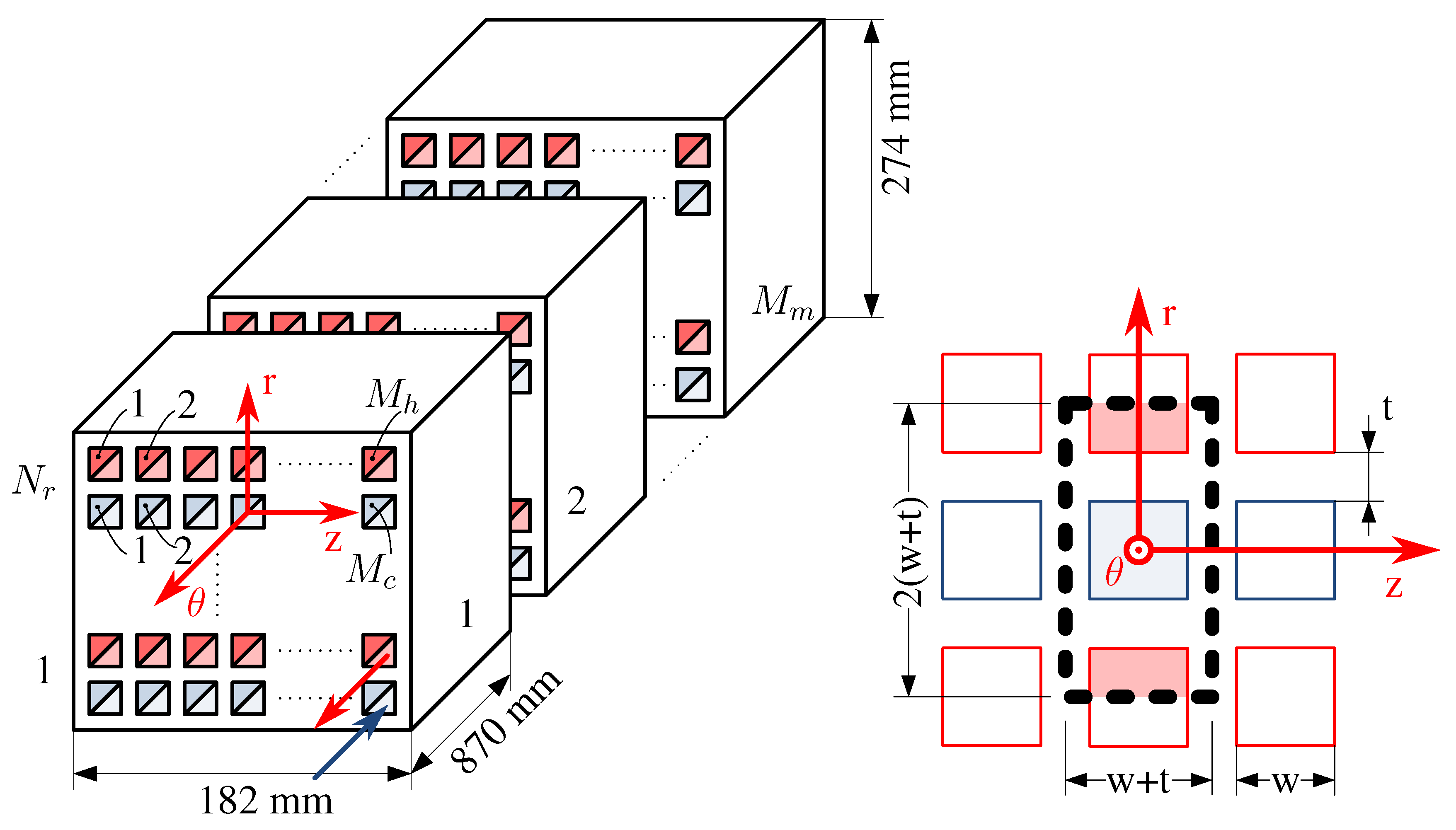
2.3.3. Regenerator

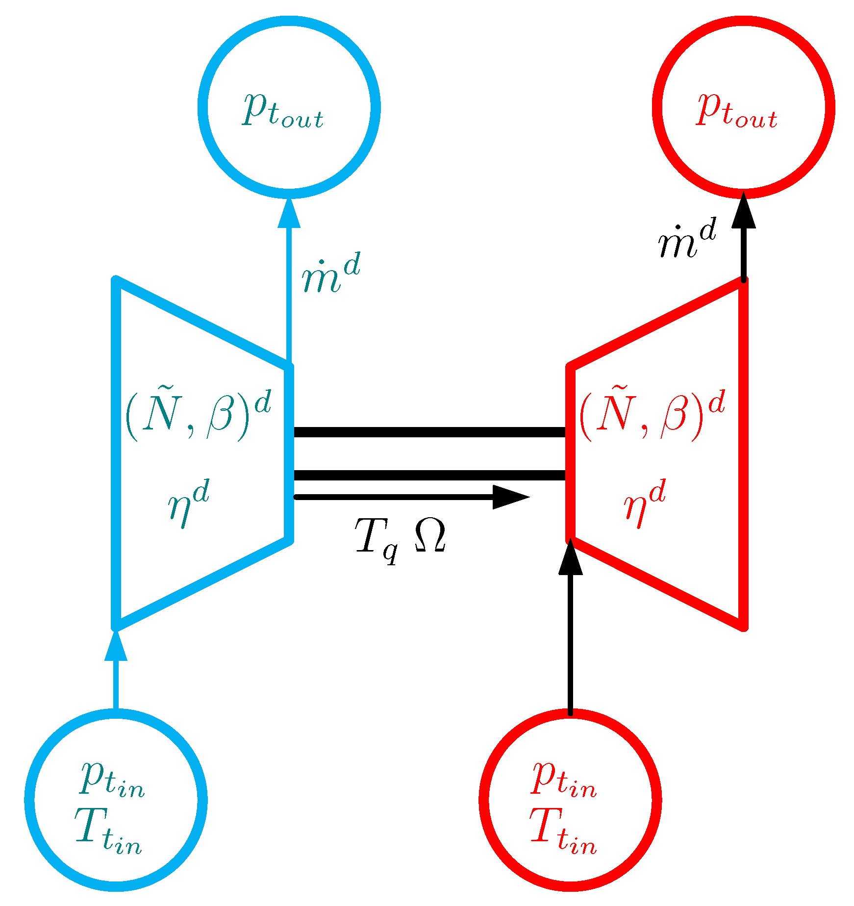
2.4. Turbomachinery

| Scaling factors | |||||||||||||
| Label | [bar] | [K] | [kg s ] | [%] | [rpm] | [hN m] | [kg m ] | ||||||
| C | 2.9 | 648 | 172.6 | 4.2 | 86 | 0.74 | 0.75 | 10,471 | 594 | 0.51 | 1.54 | 2.27 | 0.99 |
| C1 | 129.6 | 296 | 11.2 | 1.5 | 94 | 0.63 | 0.72 | 48,340 | 7 | 0.01 | 0.40 | 0.39 | 1.11 |
| C2 | 129.5 | 371 | 11.2 | 1.5 | 94 | 0.63 | 0.72 | 48,340 | 9 | 0.01 | 0.45 | 0.39 | 1.11 |
| C3 | 129.4 | 458 | 11.2 | 1.5 | 94 | 0.63 | 0.72 | 48,340 | 11 | 0.01 | 0.50 | 0.39 | 1.11 |
| C4 | 129.3 | 559 | 11.2 | 1.5 | 94 | 0.63 | 0.72 | 48,340 | 13 | 0.01 | 0.55 | 0.39 | 1.11 |
| C5 | 129.2 | 676 | 11.2 | 1.5 | 94 | 0.63 | 0.72 | 48,340 | 16 | 0.01 | 0.61 | 0.39 | 1.11 |
| C6 | 50.9 | 33 | 11.2 | 3.9 | 90 | 0.63 | 0.65 | 48,357 | 4 | 0.01 | 0.45 | 2.71 | 1.08 |
| C7 | 51.4 | 75 | 11.2 | 3.9 | 90 | 0.63 | 0.65 | 48,357 | 8 | 0.01 | 0.62 | 2.67 | 1.08 |
| C8 | 51.3 | 151 | 11.2 | 3.9 | 90 | 0.63 | 0.65 | 48,357 | 15 | 0.01 | 0.86 | 2.68 | 1.08 |
| T1 | 195.7 | 1000 | 89.6 | 1.5 | 91 | 0.20 | 1.00 | 10,471 | 594 | 0.51 | 1.03 | 1.05 | 0.96 |
| T2 | 130.1 | 863 | 22.5 | 2.5 | 89 | 0.35 | 1.00 | 48,340 | 56 | 1.00 | 2.40 | 1.00 | 1.02 |
| T3 | 130.1 | 863 | 11.1 | 2.5 | 88 | 0.35 | 1.00 | 48,357 | 27 | 1.00 | 1.18 | 1.00 | 1.01 |
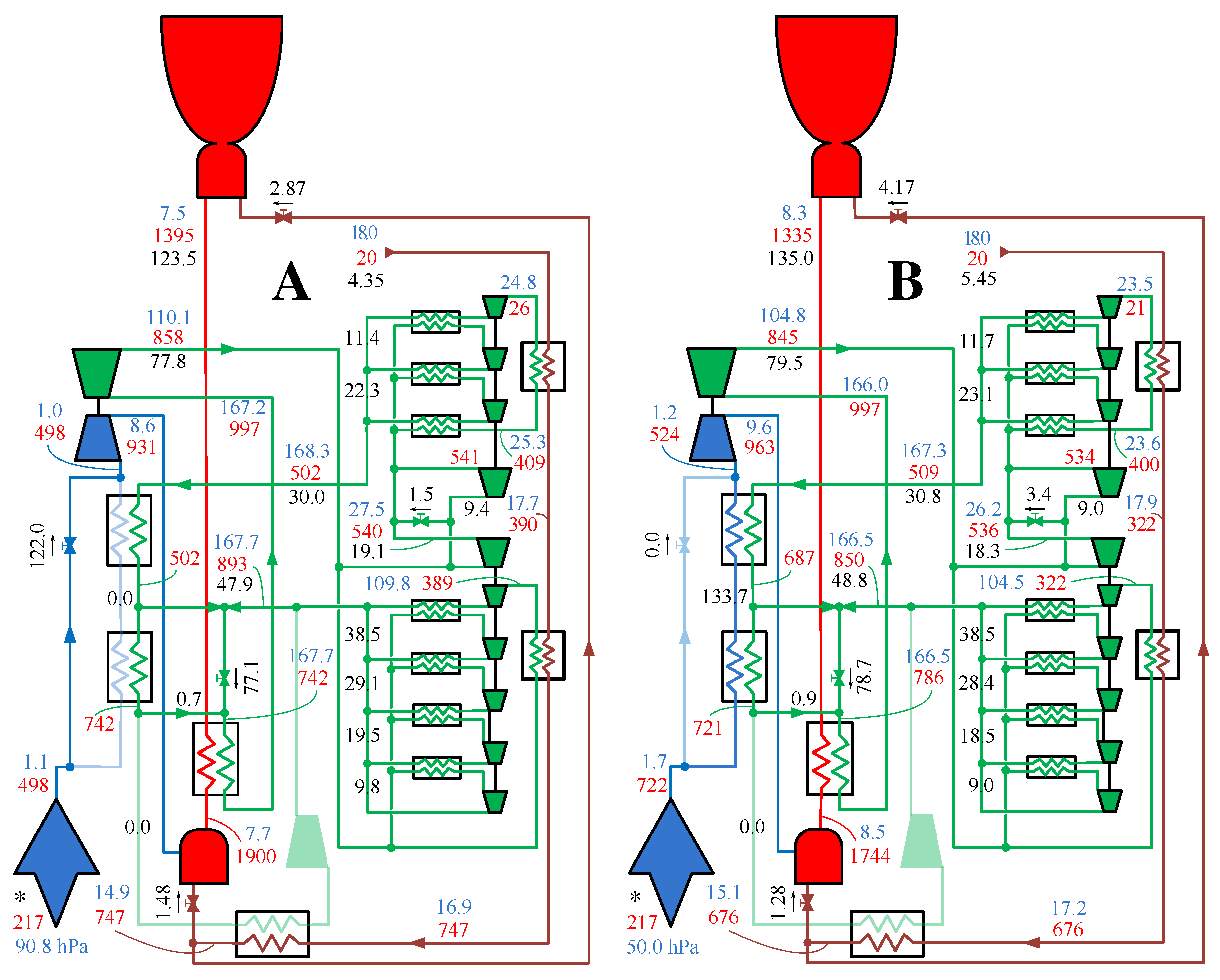
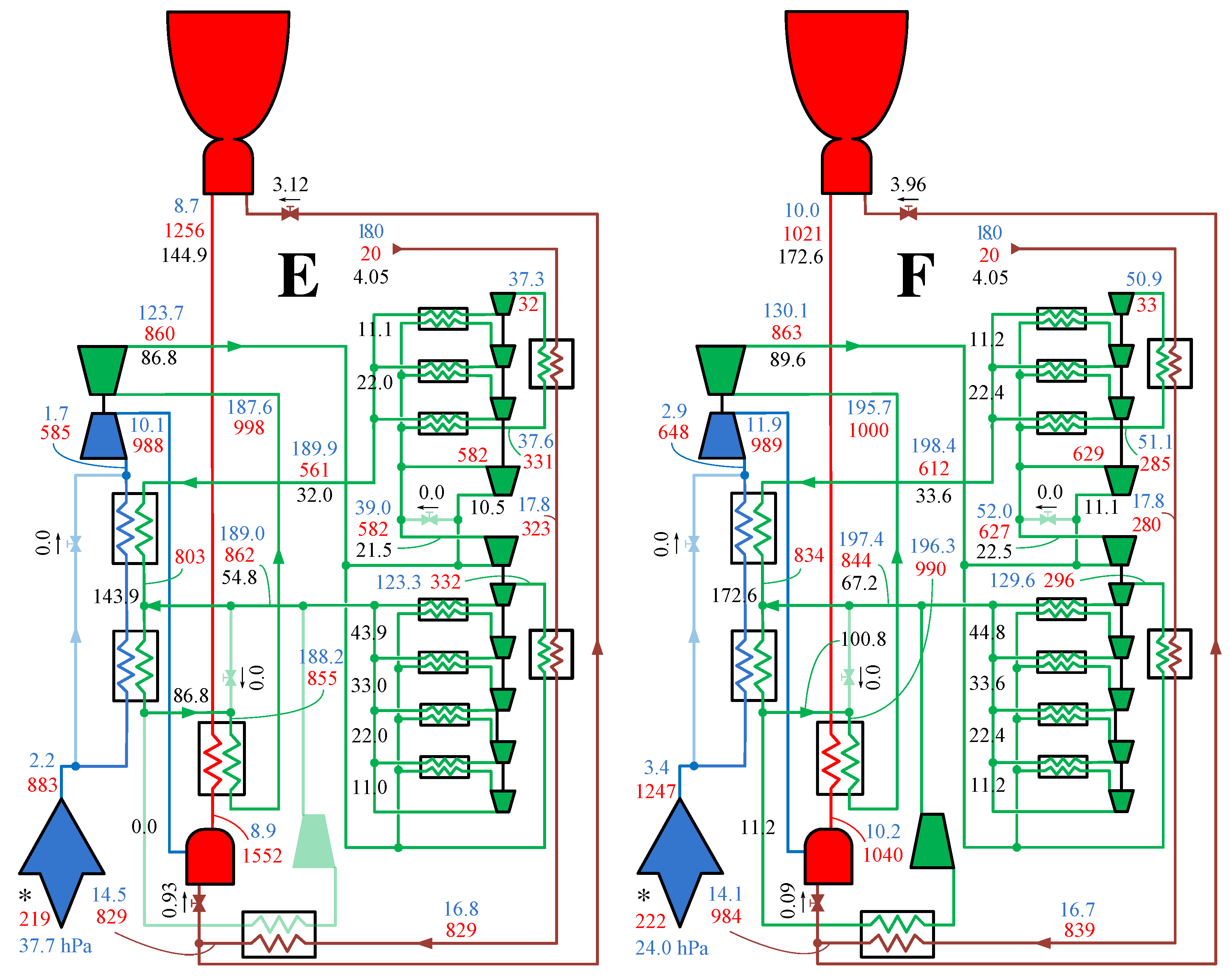
3. Engine Control
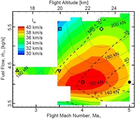
4. Results


5. Conclusions
Acknowledgements
Nomenclature:
| A | = transversal area [m] |
= cross section of the reheater helium channels [m] | |
| a | = speed of sound [m s] |
= total mass of chemical element j in the chemical species i | |
| b | = blockage ratio of the tubes in crossflow |
= total mass of chemical element j in the gas mixture | |
| C | = heat capacity [m K s] |
= specific heat at constant pressure [m K s] | |
| D | = diameter [m] |
= hydraulic diameter [m] | |
| e | = tube minimum distance to diameter ratio or total specific energy
() [m s] |
= uninstalled thrust [kg m s] | |
= mathematical function whose root defines the constraint which the turbomachinery design parameters , and must satisfy | |
| G | = Gibbs potential [kg m s] |
= mathematical function whose root defines the locus of turbomachinery operational points which satisfy the fluid dynamical constraint imposed by the turbomachine discharge duct | |
= mathematical function whose root defines the locus of turbomachinery operational points which satisfy the mechanical constraint imposed by the turbomachine shaft | |
= adiabatic efficiency characteristic of the unscaled turbomachine | |
| h | = specific enthalpy [m s] |
= convective heat transfer coefficient [kg K s] | |
= shaft inertia [kg m] | |
= specific impulse [m s] | |
| k | = thermal conductivity [kg K m s] or controller sensitivity |
= mass flow scaling factor | |
= efficiency scaling factor | |
= pressure ratio scaling factor | |
| L | = length [m] |
= characteristic length [m] | |
= axial length of the reheater module strips [m] | |
= characteristic thermal entry length [m] | |
| Ma | = Mach number |
= number of coolant channels per row in the regenerator module | |
= number of heatant channels per row in the regenerator module | |
= number of modules in each regenerator unit | |
= mass flow characteristic of the unscaled turbomachine [kg s] | |
| m | = mass [kg] |
= mass flow rate [kg s] | |
= corrected mass flow rate [Equation (38)] [kg s] | |
| N | = number of mols or rotational speed [rpm] |
= number of plates of the reheater module | |
= number of rows of heatant / coolant channels per regenerator module | |
= number of helium channels per strip of the reheater module | |
= corrected speed [Equation (37)] | |
| n | = number of nodes |
= number of strips per plate of the reheater module | |
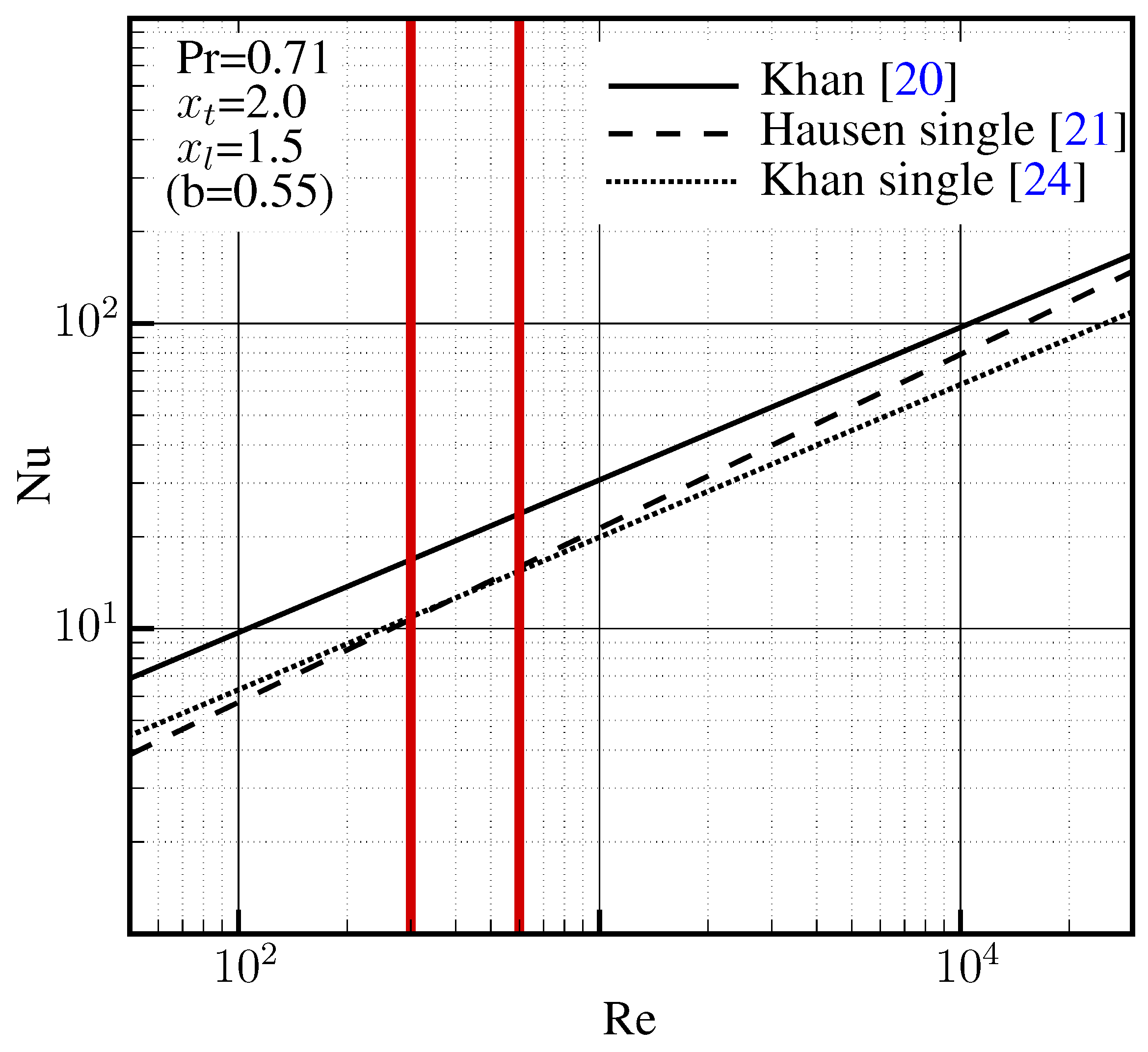
| Nu | = Nusselt number |
| Nu | = Nusselt number in turbulent flow |
| Nu | = Nusselt number in laminar fully developed flow with uniform heat flux boundary condition |
| Nu | = Nusselt number in laminar fully developed flow with isothermal boundary condition |
| Pr | = Prandtl number |
| p | = pressure [kg m s] |
= heat flux [kg s] | |
| R | = ideal gas constant [K m s] |
= curvature radius [m] | |
| Re | = Reynolds number |
| Sh | = Strouhal number |
= mathematical function whose root defines the locus of the turbomachinery steady operational points which satisfy the fluid dynamical constraint imposed by the turbomachine discharge duct | |
= mathematical function whose root defines the locus of turbomachinery operational points which satisfy the mechanical constraint imposed by the turbomachine shaft | |
| s | = tangential pitch between the reheater plates [m] |
| T | = temperature [K] |
= torque [kg m s] | |
| t | = reheater plate thickness [m] or time [s] |
= characteristic time [s] | |
| v | = velocity [m s] |
= ratio of precooler tube longitudinal pitch to external diameter | |
= ratio of precooler tube transversal pitch to external diameter |
| Greek | |
|---|---|
| β | = coordinate of the turbomachine map parametrization |
| Γ | = perimeter [m] |
| γ | = ratio of specific heats |
= increment of x | |
| δ | = dimensionless turbomachine equivalent inlet pressure () |
= rugosity [m] | |
| η | = adiabatic efficiency |
= intake kinetic efficiency | |
= nozzle efficiency | |
| Θ | = dimensionless turbomachine equivalent inlet temperature [Equation (39)] |
| λ | = tube stagger angle [rad] |
| μ | = viscosity [kg m s] |
| ξ | = friction factor [m] |
| Π | = pressure ratio characteristic of the unscaled turbomachine |
| π | = turbomachine compression (compressor) or expansion (turbine) ratio |
| ρ | = density [kg m] |
| σ | = constant of Stefan-Boltzmann [kg K s] |
| τ | = valve response time [s] |
| Ω | = rotational speed [rad s] |
| Subscripts | |
|---|---|
| c | = relative to the compressor |
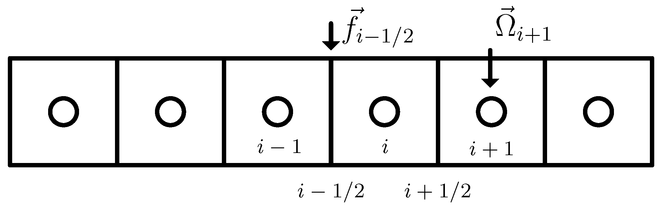
| i | = relative to the ith grid node or element in the set |
= relative to the inlet | |
= relative to the outlet | |
| s | = corresponding to an isentropic evolution |
= relative to the stream tube | |
= standard | |
| t | = stagnation quantity or relative to the turbine |
= relative to the nozzle throat | |
| w | = relative to the wall |
| ∞ | = free stream conditions |
| Superscript | |
|---|---|
= time derivative | |
= design value | |
= reference value | |
| Acronyms | |
|---|---|
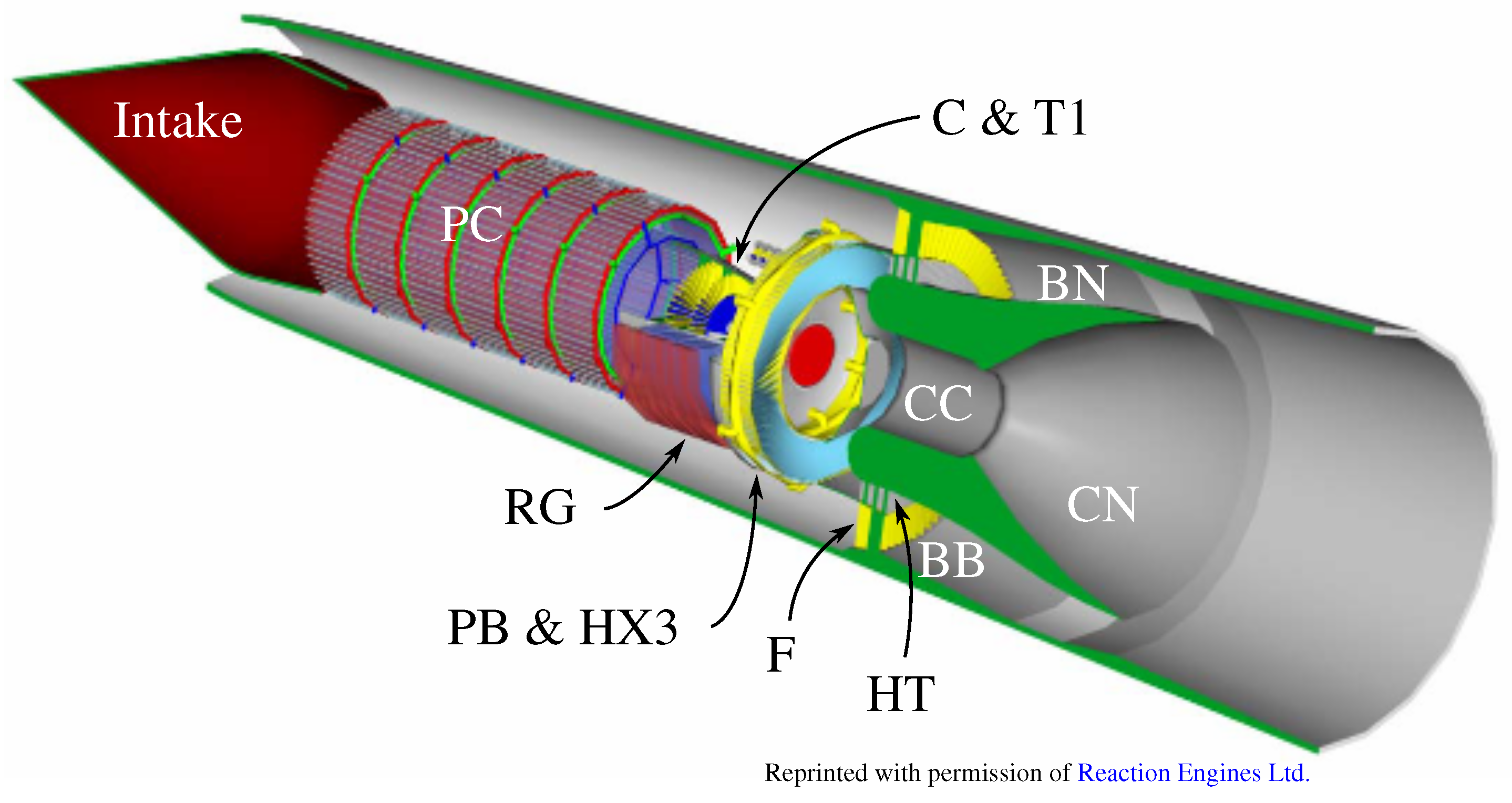
| BB | = bypass burner |
| BN | = bypass nozzle |
| CC | = main combustion chamber |
| DASSL | = differential algebraic system solver algorithm |
| ESPSS | = European Space Propulsion System Simulation |
| F | = by-pass fan |
| HT | = hub turbine |
| MR | = mixture ratio, i.e., ratio of air to fuel mass flows |
| NIST | = National Institute of Standards and Technology |
| PB | = preburner |
| PC | = precooler |
| RG | = regenerator |
| TPR | = intake total pressure recovery () |
References
- Luidens, R.W.; Weber, R.J. An Analysis of Air-Turborocket Engine Performance Including Effects of Components Changes; Technical Report RM E55H04a; NACA Lewis Flight Propulsion Laboratory: Cleveland, OH, USA, 1956. [Google Scholar]
- Escher, W.J.D. Cryogenic hydrogen-induced air-liquefaction technologies for combined-cycle propulsion applications. In Proceedings of Rocket-Based Combined-Cycle (RBCC) Propulsion Technology Workshop; NASA Lewis Research Center: Cleveland, OH, USA, March 1992; No. 92N21526. [Google Scholar]
- Balepin, V.; Tanatsugu, N.; Sato, T. Development study of precooling for ATREX engine. In Proceedings of 12th International Symposium on Air Breathing Engines; American Institute of Aeronautics and Astronautics: Melbourne, Australia, September 1995; No. ISABE 95-7015. [Google Scholar]
- Schmidt, D.K.; Lovell, T.A. Mission Performance and Design Sensitivities of Air-Breathing Hypersonic Launch Vehicles. J. Spacecr. Rocket. 1997, 34, 158–164. [Google Scholar] [CrossRef]
- Steelant, J. Sustained Hypersonic Flight in Europe: First Technology Achievements within LAPCAT II. In Proceedings of 17th AIAA International Space Planes and Hypersonic Systems and Technologies Conference; American Institute of Aeronautics and Astronautics: San Francisco, CA, USA, April 2011; No. AIAA-2011-2243. [Google Scholar]
- Jivraj, F.; Varvill, R.; Bond, A.; Paniagua, G. The Scimitar Precooled Mach 5 Engine. In Proceedings of 2nd European Conference for Aerospace Sciences (EUCASS), Brussels, Belgium, July 2007.
- Moral, J.; Pérez Vara, R.; Steelant, J.; de Rosa, M. ESPSS Simulation Platform. In Space Propulsion 2010; European Space Agency: San Sebastian, Spain, May 2010. [Google Scholar]
- Petzold, L.R. DASSL: Differential Algebraic System Solver; Technical Report; Sandia National Laboratories: Livermore, CA, USA, 1983. [Google Scholar]
- ESA; Astrium-Bremen; Cenaero; Empresarios Agrupados Int.; Kopoos. ESPSS EcosimPro Libraries User Manual; Version 2.0; Technical Report TN-4140; ESA European Space Research and Technology Centre: Noordwijk, The Netherlands, 2010. [Google Scholar]
- Gordon, S.; McBride, B.J. Computer Program for the Calculation of Complex Chemical Equilibrium Compositions with Applications; I Analysis; Technical Report RP 1311; NASA Glenn Research Center: Cleveland, OH, USA, 1994. [Google Scholar]
- Churchill, S.W. Friction-Factor Equation Spans All Fluid-Flow Regimes. Chem. Eng. 1977, 84, 91–92. [Google Scholar]
- Lemmon, E.W.; McLinden, M.O.; Friend, D.G. Thermophysical Properties of Fluid Systems. In NIST Chemistry WebBook; NIST Standard Reference Database No. 23; National Institute of Standards and Technology: Gaithersburg, MD, USA, 2007. [Google Scholar]
- Heiser, W.H. Hypersonic Airbreathing Propulsion; American Institute of Aeronautics and Astronautics: Washington, DC, USA, 1994; ISBN 1563470357. [Google Scholar]
- U.S. Standard Atmosphere, 1976; Technical Report NASA-TM-X-74335; NOAA-NASA-USAF: Washington, DC, USA, 1976.
- Bartz, D.R. Turbulent Boundary-Layer Heat Transfer from Rapidly Accelerating Flow of Rocket Combustion Gases and of Heated Air. Adv. Heat Transf. 1965, 2, 1–108. [Google Scholar]
- Martinez-Sanchez, M. Liquid Rocket Propulsion Theory. In Spacecraft Propulsion; Von Karman Institute: Rhode-Saint-Genèse, Belgium, 1993; VKI LS 1993-01. [Google Scholar]
- Varvill, R. Heat Exchanger Development at Reaction Engines Ltd. In Proceedings of 59th International Astronautical Congress; International Astronautical Federation: Glasgow, UK, September–October 2008; IAC-08-C4.5.2.
- Churchill, S.W.; Usagi, R. A general expression for the correlation of rates of transfer and other phenomena. AIChE J. 1972, 18, 1121–1128. [Google Scholar] [CrossRef]
- Bejan, A.; Kraus, A.D. Heat Transfer Handbook; Number ISBN 0-471-39015-1; John Wiley & Sons: Hoboken, NJ, USA, 2003; p. 1480. [Google Scholar]
- Khan, W.A.; Culham, J.R.; Yovanovich, M.M. Convection Heat Transfer from Tube Banks in Crossflow: Analytical Approach. Int. J. Heat Mass Transf. 2006, 49, 4831–4838. [Google Scholar] [CrossRef]
- Hausen, H. Heat Transfer in Counterflow, Parallel Flow and Cross Flow; McGraw-Hill: New York, NY, USA, 1983. [Google Scholar]
- Nakayama, A.; Kuwahara, F.; Hayashi, T. Numerical Modelling for Three-Dimensional Heat and Fluid Flow Through a Bank of Cylinders in Yaw. J. Fluid Mech. 2004, 498, 139–159. [Google Scholar] [CrossRef]
- Beale, S.B.; Spalding, D.B. A Numerical Study of Unsteady Fluid Flow in In-Line and Staggered Tube Banks. J. Fluid. Struct. 1999, 13, 723–754. [Google Scholar] [CrossRef]
- Khan, W.A.; Culham, J.R.; Yovanovich, M.M. Fluid Flow and Heat Transfer from a Cylinder Between Parallel Planes. J. Thermophys. Heat Transf. 2004, 18, 395–403. [Google Scholar] [CrossRef]
- Webber, H.; Feast, S.; Bond, A. Heat Exchanger Design in Combined Cycle Engines. In Proceedings of 59th International Astronautical Congress; International Astronautical Federation; Glasgow, UK, September–October 2008; IAC-08-C4.5.1.
- Colgan, E.G.; Furman, B.; Gaynes, M.; Graham, W.S.; LaBianca, N.C. A Practical Implementation of Silicon Microchannel Coolers for High Power Chips. IEEE Trans. Compon. Packag. Technol. 2007, 30, 218–225. [Google Scholar] [CrossRef]
- Kim, S.J.; Kim, D. Forced Convection in Microstructures for Electronic Equipment Cooling. J. Heat Transf. 1999, 121, 639–645. [Google Scholar] [CrossRef]
- Sui, Y.; Lee, P.S.; Teo, C.J. An Experimental Study of Flow Friction and Heat Transfer in Wavy Microchannels with Rectangular Cross Section. Int. J. Therm. Sci. 2011, 50, 2473–2482. [Google Scholar] [CrossRef]
- Gong, L.; Kota, K.; Tao, W.; Joshi, Y. Parametric Numerical Study of Flow and Heat Transfer in Microchannels with Wavy Walls. J. Heat Transf. 2011, 133, 051702:1–051702:10. [Google Scholar] [CrossRef]
- Riegler, C.; Bauer, M.; Kurzke, J. Some aspects of modeling compressor behavior in gas turbine performance calculations. J. Turbomach. 2001, 123, 372–378. [Google Scholar] [CrossRef]
- Dixon, S.L. Fluid Mechanics, Thermodynamics of Turbomachinery; Butterworth-Heinemann: Oxford, UK, 1998. [Google Scholar]
- Cumpsty, N. Jet Propulsion—A Simple Guide to the Aerodynamic and Thermodynamic Design and Performance of Jet Engines; Cambridge University Press: Cambridge, UK, 1997; p. 115. [Google Scholar]
- Paniagua, G.; Szokol, S.; Kato, H.; Manzini, G. Contrarotating Turbine Aerodesign for an Advanced Hypersonic Propulsion System. J. Propuls. Power 2008, 24, 1269–1277. [Google Scholar] [CrossRef]
- Kurzke, J. Component Map Collection; Joachim Kurzke: Dachau, Germany, 2004; Issue 2. [Google Scholar]
- Coverse, G.L. Extended Parametric Representation of Compressor Fans and Turbines; Technical Report NASA-CR-174646; NASA Lewis Research Center: Cleveland, OH, USA, 1984; Volume 2. [Google Scholar]
- Kurzke, J.; Riegler, C. A New Compressor Map Scaling Procedure for Preliminary Conceptual Design of Gas Turbines; ASME IGTI Turbo Expo: Munich, Germany, 2000; 2000-GT-0006. [Google Scholar]
- Brenan, K.E.; Campbell, S.L.; Petzold, L.R. Numerical Solution of Initial-Value Problems in Differential Algebraic Equations; SIAM: Philadelphia, PA, USA, 1996. [Google Scholar]
© 2013 by the authors; licensee MDPI, Basel, Switzerland. This article is an open access article distributed under the terms and conditions of the Creative Commons Attribution license (http://creativecommons.org/licenses/by/3.0/).
Share and Cite
Fernandez-Villace, V.; Paniagua, G. Numerical Model of a Variable-Combined-Cycle Engine for Dual Subsonic and Supersonic Cruise. Energies 2013, 6, 839-870. https://doi.org/10.3390/en6020839
Fernandez-Villace V, Paniagua G. Numerical Model of a Variable-Combined-Cycle Engine for Dual Subsonic and Supersonic Cruise. Energies. 2013; 6(2):839-870. https://doi.org/10.3390/en6020839
Chicago/Turabian StyleFernandez-Villace, Victor, and Guillermo Paniagua. 2013. "Numerical Model of a Variable-Combined-Cycle Engine for Dual Subsonic and Supersonic Cruise" Energies 6, no. 2: 839-870. https://doi.org/10.3390/en6020839