A Bayesian Method for Short-Term Probabilistic Forecasting of Photovoltaic Generation in Smart Grid Operation and Control

Abstract

A new short-term probabilistic forecasting method is proposed to predict the probability density function of the hourly active power generated by a photovoltaic system. Firstly, the probability density function of the hourly clearness index is forecasted making use of a Bayesian auto regressive time series model; the model takes into account the dependence of the solar radiation on some meteorological variables, such as the cloud cover and humidity. Then, a Monte Carlo simulation procedure is used to evaluate the predictive probability density function of the hourly active power by applying the photovoltaic system model to the random sampling of the clearness index distribution. A numerical application demonstrates the effectiveness and advantages of the proposed forecasting method.

1. Introduction

In recent years, power systems have been undergoing radical changes and in the near future their planning and operation will be undertaken according to the Smart Grid (SG) vision. The SG initiatives aim at introducing new technologies and services in power systems to make the electrical networks more reliable, efficient, secure and environmentally-friendly [1].

Increasing the exploitation of renewable energy sources (such as wind and solar energy) is certainly one of the most important goals of SGs. Indeed, the random behavior of such energy sources introduce challenging issues in the design of advanced tools and techniques for the optimal SG operation and control. In tackling these issues, forecasting is a fundamental task for an efficient utilization of the available distributed energy resources and for a secure and economic behaviour of the power system [2].

In general, the power system operator can use accurate forecast information about renewable power generation and load consumption to guarantee a balance between generation and demand at all the time with reduced capacity and costs of the operating reserves [3,4]. From the perspective of the producers, forecasting the renewable power output can be very useful for decision making on the energy market. In this way, not only the deviation between scheduled and actual generation can be minimized, but also the revenues are increased, thus reducing the penalties related to regulation costs and enhancing the competitiveness of renewable energies in comparison with dispatchable energy sources [5]. Finally, prosumers can use prediction models to plan their consumption patterns so as to match the power they generate on-site thus maximizing their benefits [6].

In the relevant literature, various forecasting methods have been proposed to estimate the expected power generated from a renewable energy source, which essentially differ in the type of the information characterizing the predicted output and in the time horizon of their application.

Concerning the type of information, two main forecasting methods can be adopted, referred to as deterministic and probabilistic forecasting. In the former one, a single value of the renewable power generation is provided and no uncertainty of the prediction is considered. In the latter one, the output value is accompanied with information on its intrinsic unpredictability and, then, it is more appropriate to solve problems of management and control in future SGs [3,5,7]. Probabilistic forecasting methods can be distinguished in two further categories according to the adopted approach: the prediction error or the direct approach. While the first one provides the uncertainty of the error deriving from the application of a deterministic forecasting method, the second one directly yields the statistic representation of the predicted output.

Concerning the time horizon, renewable generation forecasting can basically be divided into different time intervals, depending on the time frames corresponding to the tasks of grid operation and control and to the sessions of electricity markets. Short-term forecasting covers time intervals ranging from less than 1 hour to few hours ahead and is very useful for frequency regulation and load balancing. Medium term forecasting, up from several hours to few days ahead, is needed for unit commitment and energy trading. Finally, long-term forecasting can be required to support system planning and economic analyses in seasonal and annual horizons. However, recent renewable integration studies have shown that it is the short term forecasting that gains the most in a SG [3].

One of the most promising renewable energy conversion system to be integrated in SGs is the PhotoVoltaic (PV) power generation, due to the expected cost reduction and the increased efficiency of both PV panels and converters [8]. The power generated by a PV power system varies according to the solar radiation on the earth’s surface, which mainly depends on the installation site and the weather conditions. While the dependence on the specific location can be essentially predicted on a deterministic way, the atmospheric conditions (such as cloud cover, ambient temperature, relative humidity) are the main causes of the randomness of the solar radiation and it is very important to consider them when short-term forecasting is concerned [9,10].

Several methods have been proposed in the relevant literature for forecasting the PV power generated in a short time horizon. In [11] a recurrent neural network has been proposed to perform a short term forecasting of the PV power production using meteorological data of the last 16 days and has been compared with a feed-forward neural network. A method to predict PV power output has been presented in [12] by deriving hourly site-specific irradiance forecasts from data provided by a weather forecasts center. In [13] an advanced Grey-Markov chain model has been applied to predict the daily power production of grid-connected PV systems using operating data collected at 15 minute intervals. A two-stage method to predict hourly value of the PV power for time horizon up to 36 hours has been proposed in [14]. In [15] Kalman filters are applied to predict sub-hourly and hourly PV power production using solar irradiance as input. First studies on the application of Bayesian theory for PV power production forecasting are shown in [16,17].

In this paper, extending and improving the approach based on the Bayesian theory outlined in [16,17,18], a new method for short-term probabilistic forecasting is proposed, that directly yields to the statistic representation of the predicted PV power output. The proposed method forecasts at the generic hour $h$ the probability density function (pdf) of the active power produced by a PV power system at the hour $h+k$ with $k=1,\mathrm{...}, K$, starting from the evaluation of samples of the pdf of the hourly clearness index at hour $h+k$. The forecast of the pdf of the hourly clearness index is obtained firstly selecting for the pdf an analytical expression and, then, evaluating the pdf parameters by applying the Bayesian Inference (BI). To this aim, an Auto Regressive (AR) time series model, representing the relationship between the pdf parameters, the clearness index and some explanatory meteorological variables, is used together with appropriate sets of historical measurements of the random variables involved in the AR model. Finally, a Monte Carlo (MC) simulation procedure is applied to generate the predicted pdf of the PV active power: a random sampling of the pdf of the hourly clearness index is performed and, using the PV system model, the PV power samples are obtained.

The key steps of the proposed method are: (i) the choice of the analytical expression of the pdf modeling the hourly clearness index; (ii) the definition of an adequate AR time series model so as to consider only the meteorological variables that most affect the hourly clearness index behaviour; and (iii) the selection of appropriate data vectors from historical measurements collected before the time of the forecast.

The peculiarity of the method is that it takes into account the dependence of the terrestrial solar radiation on some explanatory atmospheric variables and combines probabilistic techniques, such as BI and MC simulation, to provide a probabilistic forecasting of the PV power generation useful for optimal SG operation and control.

This paper is organized as follows: Section 2 briefly recalls the probabilistic forecasting method based on the Bayesian approach. In Section 3 the probabilistic method is applied to forecast the power production of a PV system. Finally, numerical simulations are reported in Section 4 to give evidence of the effectiveness of the proposed approach.

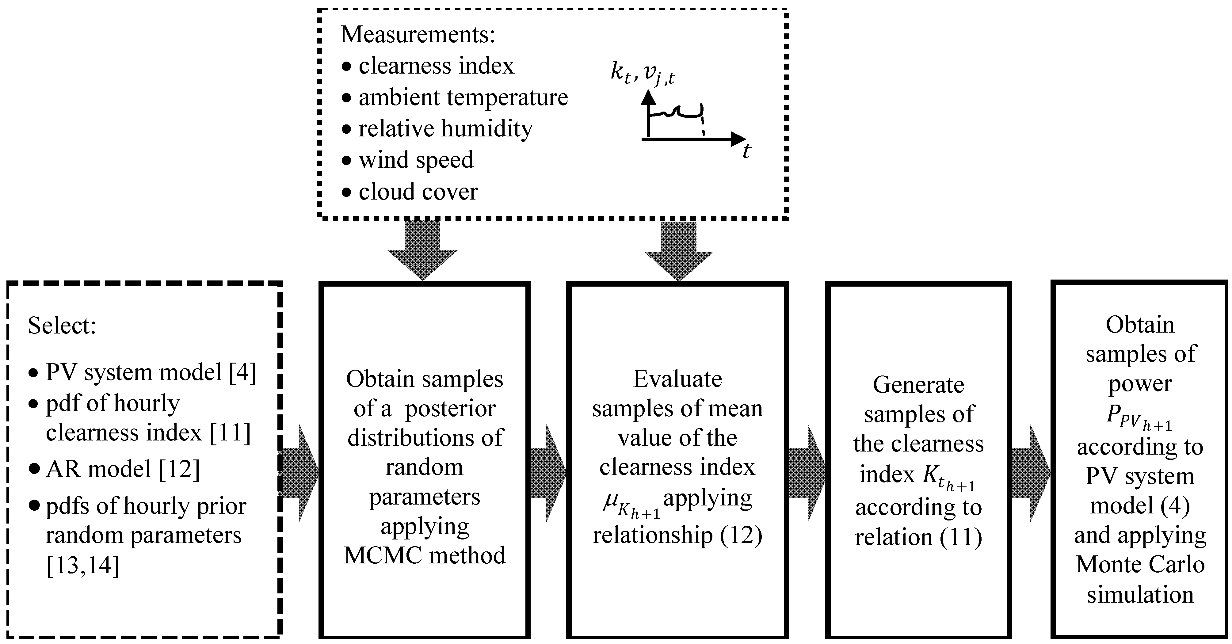
2. Probabilistic Forecasting method based on the Bayesian approach

The probabilistic forecasting method based on the Bayesian approach predicts at the generic hour $t=h$ the pdf of a random variable $X_t$ at the hour $t=h+k$, with $k=1,\dots ,\text{ K}$. For the sake of simplicity, in the following the analysis is referred to the case of $k=1$.

In applying this method, the starting point is the knowledge of the analytical expression of the pdf $f_{X_t}\left(X_t\right)$ of the random variable to be forecasted. Usually, the analytical expression of the pdf is characterized by some distribution parameters and it is modeled as a conditional pdf. For the sake of conciseness, reference is made to only one distribution parameter (i.e., the mean value), generically referred to as ${\vartheta }_t$, and the conditional pdf is indicated as $f_{X_t}(X_t|{\vartheta }_{t })$.

Forecasting at $t=h$ the pdf $f_{X_{hh+1}}(X_{h+1}\text{|}{\vartheta }_{h+1 })$ requires an estimation of ${\vartheta }_{h+1}$. To this aim, a first order AR time series model can be used, representing the relationship between ${\vartheta }_{h+1}$ and both the measurements $x_h$ and ($v_{1,h},\dots , v_{M,h})$ collected at the hour $h$ of, respectively, the random variable $X_t$ to be forecasted and the $M$ explanatory random variables $V_{1,t},\dots , V_{M,t}$ influencing $X_t$:

$${\vartheta }_{h+1}={\alpha }_1{x}_h+{\beta }_1{v}_{1,h}+ \mathrm{...} + {\beta }_M{v}_{M,h}+ {\alpha }_0$$

(1)

where ${\alpha }_0, {\alpha }_1, {\beta }_1,\dots , {\beta }_M$ are the coefficients of the AR model. Explanatory variables are variables such that changes in their value are thought to cause changes in another variable.

In the classical statistics, ${\alpha }_0, {\alpha }_1, {\beta }_1,\dots , {\beta }_M$ are assumed to be constant. Indeed, when Bayesian approach are adopted, such coefficients are modeled as random variables, known as prior random parameters, and the BI [19] allows to estimate the conditional pdf $p({\alpha }_0, {\alpha }_1, {\beta }_1,\dots , {\beta }_M| {\mathit{S}}_{{\mathit{X}}_{\mathit{h}}})$ of the parameters ${\alpha }_0, {\alpha }_1, {\beta }_1,\dots , {\beta }_M$ given the set ${\mathit{S}}_{{\mathit{X}}_{\mathit{h}}}=(x_{s_1}, \mathrm{...} , x_{s_{N_h}})$ composed of $N_h$ measurements of $X_t$ observed before the hour $h$. The pdf $p({\alpha }_0, {\alpha }_1, {\beta }_1,\dots , {\beta }_M| {\mathit{S}}_{{\mathit{X}}_{\mathit{h}}})$ is known as a posteriori distribution of the prior random parameters and it is very difficult to obtain its expression in closed form. Actually, only a simplified expression, known as unnormalized a posteriori distribution of the prior random parameters, and indicated as $q({\alpha }_0, {\alpha }_1, {\beta }_1,\dots , {\beta }_{M }\text{|} {\mathit{S}}_{{\mathit{X}}_{\mathit{h}}}\text{)},$ can be provided. Fortunately, the knowledge of the unnormalized a posteriori distribution of the prior random parameters is sufficient for developing algorithms that provide information about the normalised a posteriori distributions.

The unnormalized a posteriori distribution of the prior random parameters is derived from the application of the Bayes’ rule assuming the independency of the prior random parameters so that:

$$q({\alpha }_0, {\alpha }_1, {\beta }_1,\dots , {\beta }_{M }|{\mathit{S}}_{{\mathit{X}}_{\mathit{h}}})= p({\mathit{S}}_{{\mathit{X}}_{\mathit{h}}}\text{|}{\alpha }_0, {\alpha }_1, {\beta }_1,\dots , {\beta }_{M }) {{\displaystyle \prod }}_{i=0}^{1}p({\alpha }_i){{\displaystyle \prod }}_{j=1}^{M}p({\beta }_j)$$

(2)

where $p({\mathit{S}}_{{\mathit{X}}_{\mathit{h}}}\text{|}{\alpha }_0,{\alpha }_1,{\beta }_1,\dots ,{\beta }_M)$ is the likelihood function; and $p({\alpha }_i)$ and $p({\beta }_j)$ are the a priori distributions of the prior random parameters.

The a priori distributions are the initial pdfs of the prior random parameters which are not conditional on observed data. Their expressions can be vague or informative and reflects the knowledge that we have in advance about the pdfs that we are interested in.

The likelihood function is the conditional data distribution, that is the pdf modeling $X_t$, whose realizations are contained in ${\mathit{S}}_{{\mathit{X}}_{\mathit{h}}}$, given the prior random parameters. Its expression can be derived making use of the $f_{X_t}(X_t\text{|}{\vartheta }_{t })$ for the set ${\mathit{S}}_{{\mathit{X}}_{\mathit{h}}}$ and assuming that $x_{s_1}, \mathrm{...} , x_{s_{N_h}}$ are independent realizations of $X_t$. Substituting for ${\vartheta }_t$ the AR time series model and using the vectors ${\mathit{S}}_{{\mathit{V}}_{\mathbf{1},\mathit{h}}}=\left(v_{1,s_1}, \mathrm{...}, v_{1,s_{N_h}}\right)$, … , ${\mathit{S}}_{{\mathit{V}}_{\mathit{M},\mathit{h}}}=\left(v_{M,s_1}, \mathrm{...} , v_{M, s_{N_h}}\right)$ of the $N_h$ measurements of the explanatory variables $V_{1,t},\dots , V_{M,t}$ corresponding to ${\mathit{S}}_{{\mathit{X}}_{\mathit{h}}}$, it obtains:

$$p({\mathit{S}}_{{\mathit{X}}_{\mathit{h}}}\text{|}{\alpha }_0, {\alpha }_1, {\beta }_1,\dots , {\beta }_{M })= {{\displaystyle \prod }}_{i=2}^{N_h}{f}_{X_t}(x_{s_i}\text{|}{\vartheta }_{s_i }={\alpha }_1{x}_{s_i-1}+{\beta }_1{v}_{1,s_i-1}+ \mathrm{...} + {\beta }_M{v}_{M,s_i-1}+ {\alpha }_0)$$

(3)

Once the unnormalized a posteriori distribution of the prior random parameters is known, it is trivial to evaluate the normalised a posteriori distributions of each parameter by applying the theory of the joint pdfs [20]. Then, the Monte Carlo Markov Chain (MCMC) simulation method based on the Metropolitan-Hasting algorithm [21] can be directly applied to the unnormalized distributions of every parameter to obtain samples of their a posteriori distributions. In the MCMC approach, a Markov chain is constructed, characterized by a transition probability matrix reflecting the a posteriori distributions of the prior random parameters. Then, the Markov chain is simulated until the samples are representative of the a posteriori distributions of every parameter.

Eventually, incorporating the AR time series model in this procedure, the samples derived from the a posteriori pdfs of ${\alpha }_0, {\alpha }_1, {\beta }_1,\dots , {\beta }_M$ can be used together with the measurements $x_h$ and $v_{1,h},\dots , v_{M,h}$ collected at the hour $h$ to obtain samples of ${\vartheta }_{h+1}$. Finally, for each simulated sample of ${\vartheta }_{h+1}$, the samples of the random variable $X_t$ are drawn from the analytical expression of the pdf so as to provide the full predictive distribution $f_{X_{hh+1}}(X_{h+1}\text{|}{\vartheta }_{h+1 })$.

3. Probabilistic Forecasting of the Photovoltaic Generation

In the following, the probabilistic forecasting method described in Section 2 is applied to predict at hour $h$ the pdf of the PV power production at hour $h+1$, starting from an estimation of the terrestrial hourly solar radiation, expressed in terms of the pdf of the hourly clearness index at hour $h+1$. The next four subsections dealt with:

–

The description of the adopted model for the PV system;

–

The description of the pdf modeling the hourly clearness index;

–

The definition of the AR time-series model including meteorological variables; and

–

The probabilistic characterization of the prior random parameters.

3.1. PV System Model

The hourly active power produced by a PV system depends on the availability of the solar radiation at the installation site. The solar radiation in a given locality cannot be exactly predicted owing mainly to the irregular presence of clouds. The sky conditions are often taken into account by representing the terrestrial solar radiation in terms of clearness index that is defined as the ratio of the surface radiation to the extraterrestrial radiation for a given period [22].

When the PV system is equipped with a maximum power point tracker, an analytical relationship exists between the PV active power $P_{P{V}_t}$ at the hour $t$ and the corresponding hourly clearness index $K_t$, [22,23,24] that is defined as the ratio of the hourly total solar radiation on an horizontal plane I_t to the extra-terrestrial hourly total solar radiation I₀; it results:

$$P_{P{V}_t}=S_C\mathsf{\eta } \left(T{K}_t-T^{\prime }{K}_t^2\right)$$

(4)

where $S_C$ is the array surface area; η is the efficiency of the PV system; and $T$ and $T^{\prime }$ are defined as:

$$T=\left[\left(R_b+\rho \frac{1-\cos \gamma }{2}\right)+\left(\frac{1+\cos \gamma }{2}-R_b\right)p\right]r_d\frac{H_0}{3600}$$

(5)

$$T^{\prime }=\left(\frac{1+\cos \gamma }{2}-R_b\right)q{r}_d\frac{H_0}{3600}$$

(6)

where $R_b$ is the ratio of beam radiation on a tilted surface to that on a horizontal surface at any time; ρ is the reflectance of the ground; γ is the inclination of the array surface to the horizontal plane; $r_d$ is the ratio between diffuse radiation in hours and diffuse radiation in a day; $H_o$ is the extra-terrestrial total solar radiation; and $p, q$ are coefficients reported in [23], which link the diffuse fraction of the hourly total solar radiation on horizontal plane with the hourly clearness index.

The analysis of the relationship (4) clearly reveals that $K_t$ is the only variable affecting $P_{P{V}_t}$, once the hour of the day, the installation site and the technical characteristics of the PV system are assigned. The hourly clearness index $K_t$ is a random variable modelling the uncertain behaviour of the terrestrial solar radiation. The hourly PV active power $P_{P{V}_t}$, as function of $K_t$, is itself a random variable and its pdf can be determined by the pdf of the hourly clearness index.

In this paper, a MC simulation procedure is used to generate at the hour $t=h$ samples of the predictive pdf of the hourly PV active power $f_{P_{P{V}_{h+1}}}\left(P_{P{V}_{h+1}}\right)$ by performing a random sampling of the pdf of the hourly clearness index $f_{K_{h+1}}\left(K_{h+1}\right)$ estimated for the hour $t=h+1$ and applying Equation (4).

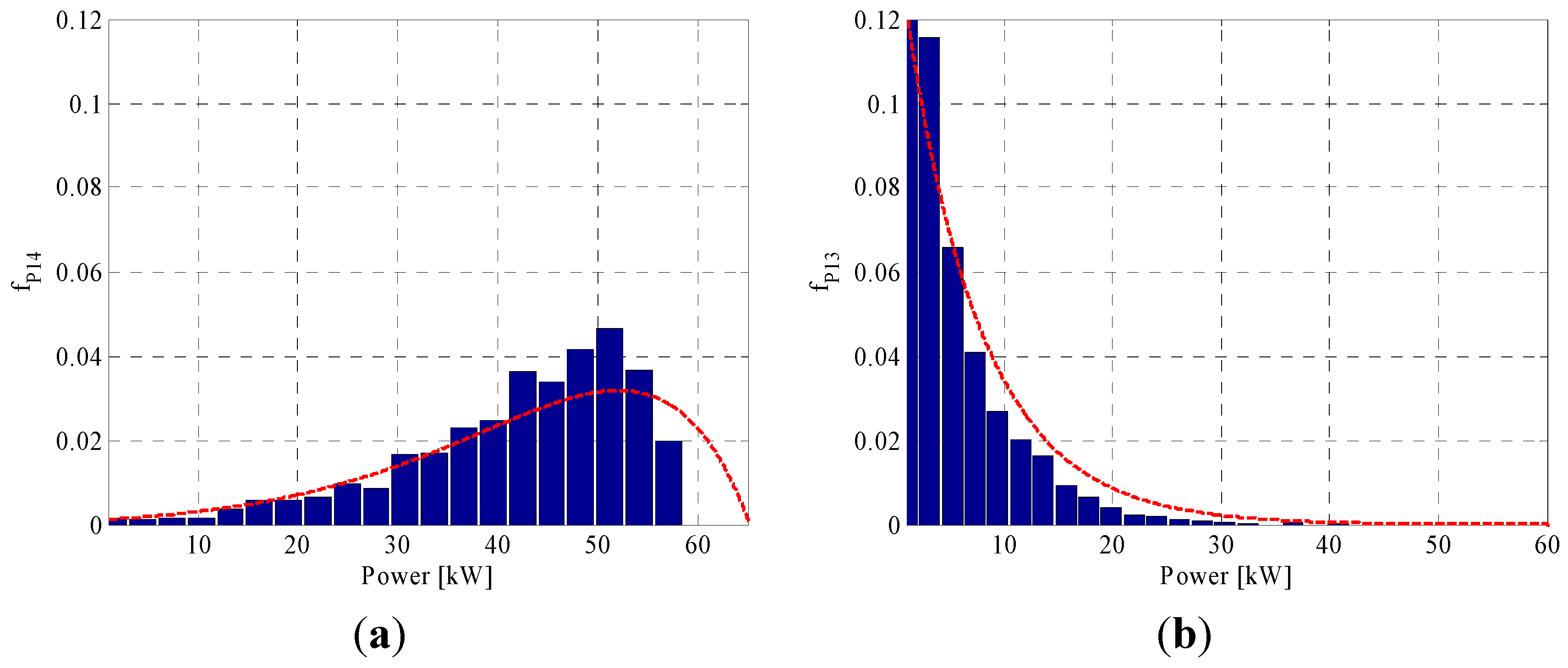
3.2. Probability Density Function of the Hourly Clearness Index

The analytical expression of the pdf of the hourly clearness index can be experimentally obtained by a statistical analysis of historical solar measurements collected in the site in which the PV system is installed. In the literature, starting from the fitting of the hourly clearness index data collected in a specific location, the investigation has often resulted in the individuation of pdfs characterized by standard distributions. In [25] the hourly clearness index measurements recorded at various locations in Algeria are conveniently described by Beta distributions. In [26] bimodal distributions are considered more adequate to model clear and cloudy sky conditions of hourly clearness index measurements collected in different cities in the U.S.A. On the other hand, several attempts have been made to find universal standard pdfs that are independent of the location and the time period used to define the clearness index [27,28,29]. Following the latter approach, in this paper the model proposed in [29] has been adopted and the following modified Gamma distribution $f_{K_t}(K_t|C_t,{\lambda }_t)$ is used to model the pdf of the hourly clearness index $K_t$:

$$f_{K_t}(K_t|C_t,{\lambda }_t)=C_t\frac{{\overline{k}}_u-K_t}{{\overline{k}}_u}{e}^{{\lambda }_t{K}_t}$$

(7)

where ${\overline{k}}_u$ is the upper bound of the observed values of $K_t$; and $C_t$ and ${\lambda }_t$ are the distribution parameters, defined as:

$$C_t=\frac{{\lambda }_t^2{\overline{k}}_u}{\left(e^{{\lambda }_t{\overline{k}}_u}-1-{\lambda }_t{\overline{k}}_u\right)}$$

(8)

$${\lambda }_t=\frac{\left(2F_t-17.519e^{-1.3118F_t}-1062e^{-5.0426F_t}\right)}{{\overline{k}}_u}$$

(9)

with:

$$F_t=\frac{{\overline{k}}_u}{{\overline{k}}_u-{\mu }_{K_t}}$$

(10)

where ${\mu }_{K_t}$ is the mean value of the hourly clearness index $K_t$ at hour $t$. Assuming the knowledge of ${\overline{k}}_u$, the distribution parameters $C_t$ and ${\lambda }_t$ only depend on the mean value ${\mu }_{K_t}$ and the pdf in Equation (7) can be rewritten as:

$$f_{K_t}\left(K_t\text{|}{\mu }_{K_t}\right)= C_t\left({\mu }_{K_t}\right)\frac{{\overline{k}}_u-K_t}{{\overline{k}}_u}{e}^{{\lambda }_t\left({\mu }_{K_t}\right)K_t}$$

(11)

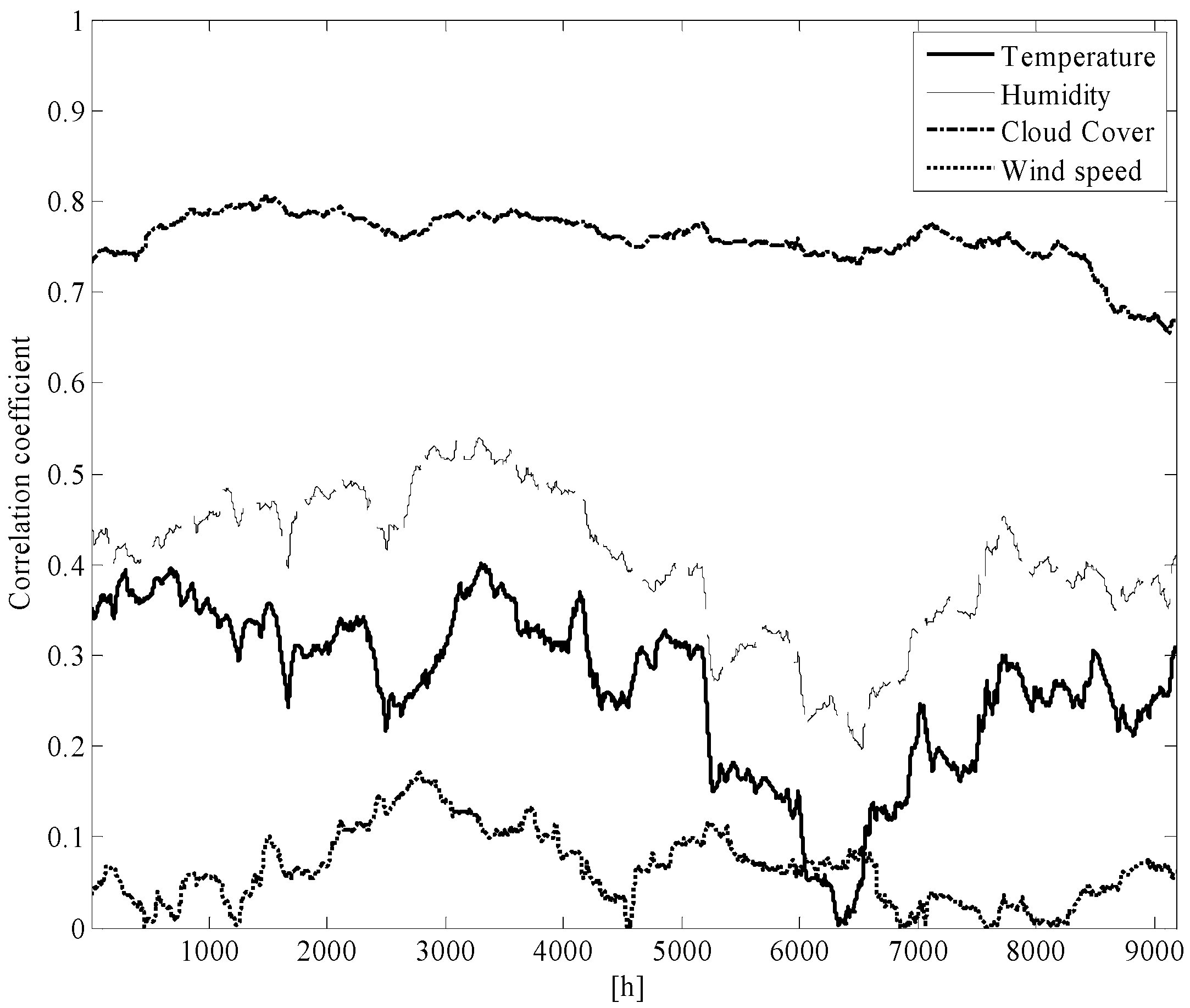
3.3. AR Time-Series Model

To predict at the hour $t=h$ the pdf $f_{K_{hh+1}}(K_{h+1}\text{|}{\mu }_{K_{h+1}})$ at the hour $t=h+1$ an estimation of the mean value ${\mu }_{K_{h+1}}$ is required, as shown in the Subsection 3.2. To this aim, an AR time series model can be used to define the relationship among such mean value and the measurements of the clearness index and of some meteorological variables influencing the solar radiation, such as the ambient temperature $AT$, the relative humidity $RH$, the wind speed $WS$ and the cloud cover $CC$, where the cloud cover is defined as the ratio in % of the sky hidden by all visible cloud. In this paper, the following first order AR time series model is adopted:

$${\mu }_{K_{h+1}}={\alpha }_1{k}_h+{\beta }_{1}a{t}_h+{\beta }_{2}r{h}_h+{\beta }_{3}w{s}_h+ {\beta }_{4}c{c}_h+{\alpha }_0$$

(12)

where $k_h$, $a{t}_h, r{h}_h,w{s}_h, c{c}_h$ are the measurements of, respectively, the clearness index, the ambient temperature, the relative humidity, the wind speed and the cloud cover, which are collected at the hour $t=h$.

The inclusion of meteorological variables in the AR model significantly increases the computational efforts in the application of the proposed forecasting method. Despite of the highest complexity of the procedure, taking into account the dependence of the clearness index on the meteorological variables allows to perform a more accurate forecasting [10,30]. To reduce computational efforts, a correlation analysis can help to individuate the meteorological variables presenting the highest influence on the solar radiation. Such analysis is performed “off-line” and correlates historical measurements collected in the specific site in which the PV system is installed. In this way, only the meteorological variables presenting the highest correlation value with the clearness index are selected so as to found a good compromise between results’ accuracy and computational efforts.

3.4. Probabilistic Characterization of the Prior Random Parameters

In this paper, the coefficients ${\alpha }_0, {\alpha }_1, {\beta }_1,{\beta }_{2, }{\beta }_3, {\beta }_4$ of the AR time series model in Equation (12) are assumed to be the prior random parameters of the BI. The a priori pdfs of the prior random parameters $p\left({\alpha }_0\right),p\left({\alpha }_1\right),p({\beta }_1),p\left({\beta }_2\right),p\left({\beta }_3\right), p\left({\beta }_4\right)$ are usually chosen with a large variance so that the data, rather than the a priori distributions, determine the relevant parameters values in the a posteriori distributions [19,20,21]. In this paper the a priori pdfs are assumed to be Gaussian with a mean value $\mu =0.5$ and a standard deviation $\sigma =0.5$ so as:

$$p\left({\alpha }_i\right)=\frac{1}{\sigma \sqrt{2\pi }}{e}^{\frac{{\left(\mu -{\alpha }_i\right)}^2}{2{\sigma }^2}} = \frac{1}{0.5\sqrt{2\pi }}{e}^{\frac{-{\alpha }_i^2}{2{\left(0.5\right)}^2}} i=0,1$$

(13)

$$p\left({\beta }_j\right)= \frac{1}{\sigma \sqrt{2\pi }}{e}^{\frac{{\left(\mu -{\beta }_j\right)}^2}{2{\sigma }^2}}=\frac{1}{0.5\sqrt{2\pi }}{e}^{\frac{-{\beta }_j^2}{2{\left(0.5\right)}^2}} j=1, \dots , 4$$

(14)

The likelihood function $p({\mathit{S}}_{{\mathit{K}}_{\mathit{h}}}\text{|}{\alpha }_0,{\alpha }_1,{\beta }_1,{\beta }_2,{\beta }_3,{\beta }_4)$ is the pdf in Equation (11) specified for the set ${\mathit{S}}_{{\mathit{K}}_{\mathit{h}}}=\left(k_{s_1},\mathrm{...},k_{s_{i}h},\mathrm{...},k_{s_{N_h}}\right)$ of $N_h$ measurements of $k_t$ observed before the hour $h$:

$$p({\mathit{S}}_{{\mathit{K}}_{\mathit{h}}}\text{|}{\alpha }_0, {\alpha }_1, {\beta }_1,{\beta }_2,{\beta }_3, {\beta }_{4 })= {{\displaystyle \prod }}_{i=2}^{N_h}{f}_{K_t}(k_{s_i}\text{|}{\mu }_{K_{si}})={{\displaystyle \prod }}_{i=2}^{N_h}C\left({\mu }_{K_{s_i}}\right)\frac{{\overline{k}}_u-k_{s_i}}{{\overline{k}}_u}{e}^{\lambda \left({\mu }_{K_{s_i}}\right)k_{s_i}}$$

(15)

where:

$${\mu }_{K_{s_i}}= {\alpha }_1{k}_{s_i-1}+{\beta }_{1}a{t}_{s_i-1}+{\beta }_{2}r{h}_{s_i-1}+{\beta }_{3}w{s}_{s_i-1}+ {\beta }_{4}c{c}_{s_i-1}+{\alpha }_0$$

(16)

Relationship (15) is obtained by substituting for ${\mu }_{K_{s_i}}$ the AR time series model in Equation (16). The generic measurements $k_{s_{i-1}}, a{t}_{s_{i-1}}, r{h}_{s_{i-1}},w{s}_{s_{i-1}}, c{c}_{s_{i-1}}$ are contained in the sets ${\mathit{S}}_{{\mathit{K}}_{\mathit{h}}}=\left(k_{s_1}, \mathrm{...},k_{s_i},\mathrm{...}, k_{s_{N_h}}\right)$, ${\mathit{S}}_{\mathit{A}{\mathit{T}}_{\mathit{h}}}=\left(a{t}_{s_1},\mathrm{...},a{t}_{s_i},\mathrm{...},a{t}_{s_{N_h}}\right)$, ${\mathit{S}}_{\mathit{R}{\mathit{H}}_{\mathit{h}}}=\left(r{h}_{s_1},\mathrm{...},r{h}_{s_i},\mathrm{...},r{h}_{s_{N_h}}\right)$, ${\mathit{S}}_{\mathit{W}{\mathit{S}}_{\mathit{h}}}=\left(w{s}_{s_1},\mathrm{...},w{s}_{s_i},\mathrm{...},w{s}_{s_{N_h}}\right)$, ${\mathit{S}}_{\mathit{C}{\mathit{C}}_{\mathit{h}}}=\left(c{c}_{s_1},\mathrm{...},c{c}_{s_i} ,\mathrm{...},c{c}_{s_{N_h}}\right)$, including $N_h$ measurements collected before the hour $h$ of, respectively, the clearness index and the meteorological variables.

According to Equation (2), the a posteriori unnormalized distribution $q\left({\alpha }_0,{\alpha }_1, {\beta }_1,{\beta }_2,{\beta }_3, {\beta }_{4 }, {\mathit{S}}_{{\mathit{K}}_{\mathit{h}}}\right)$ of the prior random parameters is equal to

(17)

and the samples of the individual a posteriori distributions are evaluated by applying the MCMC simulation method based on the Metropolitan-Hasting algorithm. The samples of the a posteriori pdfs of ${\alpha }_0,{\alpha }_1, {\beta }_1,{\beta }_2,{\beta }_3, {\beta }_{4 }$ are used in Equation (12) together with the measurements $k_h,t_h, r_h,w_h, c{c}_h$ collected at the hour $h$ to provide samples of the mean value ${\mu }_{K_{h+1}}$. Finally, for each samples of ${\mu }_{K_{h+1}}$, the samples of the hourly clearness index $X_{h+1}$ are drawn from the analytical expression of the pdf in Equation (11). The simulated samples of $X_{h+1}$ describes the predictive distribution $f_{K_{h+1}}(K_{h+1}|{\mu }_{K_{h+1}})$.

It should be noted that the choice of the measurements contained in the sets ${\mathit{S}}_{{\mathit{K}}_{\mathit{h}}}, {\mathit{S}}_{\mathit{A}{\mathit{T}}_{\mathit{h}}}, {\mathit{S}}_{\mathit{R}{\mathit{H}}_{\mathit{h}}}, {\mathit{S}}_{\mathit{W}{\mathit{S}}_{\mathit{h}}, } {\mathit{S}}_{\mathit{C}{\mathit{C}}_{\mathit{h}}}$ represent a key issue in the BI, since they are used to make inference about the prior random parameters ${\alpha }_0,{\alpha }_1, {\beta }_1,{\beta }_2,{\beta }_3, {\beta }_{4 }$. In general, these sets contain $N_h$ measurements recorded before the hour $h$ of the forecast. Actually, these data are not necessarily the ones collected from the hour $h-1$ to $h-N_h-1$, but can be selected with adequate criteria thus improving the accuracy of the proposed forecasting method. In [16] the homologue and the coded group criteria have been proposed. In the first one, the sets contain measurements at the hour $h$ which are collected $N_h$ days before the forecast (e.g., if the forecast has to be performed at h = 10:00, the sets include measurements recorded $N_h$ days before at 10:00). In the second one, the sets contain a coded group of measurements around the hour $h$ collected some days before the forecast (e.g. if the forecast has to be performed at h = 10:00, the sets include measurements from the 8:00 to 10:00 recorded $N_h/3$ days before). In addition, the measurements contained in ${\mathit{S}}_{{\mathit{K}}_{\mathit{h}}}, {\mathit{S}}_{\mathit{A}{\mathit{T}}_{\mathit{h}}}, {\mathit{S}}_{\mathit{R}{\mathit{H}}_{\mathit{h}}}, {\mathit{S}}_{\mathit{W}{\mathit{S}}_{\mathit{h}}, } {\mathit{S}}_{\mathit{C}{\mathit{C}}_{\mathit{h}}}$ can be collected at time intervals different from an hour. In [17] the data of the clearness index and of the meteorological variables contained in the vectors are extracted from measurements registered at time intervals of 15 minutes. If this is the case, the application of the proposed forecasting method will provide at the hour $h$ the predictive distribution of the clearness index at the first 15 minutes of the hour $h+1$. To estimate the pdf at the hour $h+1$ the following approach is adopted in this paper:

$$f_{K_{h+1}}\left(K_{h+1}\text{|}{\mu }_{K_{h+1}}\right)=f_{K_{h+{15}^{\prime }}}(K_{h+{15}^{\prime }}|{\mu }_{K_{h+{15}^{\prime }}})$$

(18)

that is the pdf forecasted at $h+1$ is assumed to be equal to the pdf forecasted at the first 15 minutes of the hour $h+1$. Eventually, Figure 1 shows a block diagram describing the main steps applied in the proposed Bayesian approach.

Figure 1. Block diagram describing the main steps applied in the proposed Bayesian approach.

Figure 1. Block diagram describing the main steps applied in the proposed Bayesian approach.

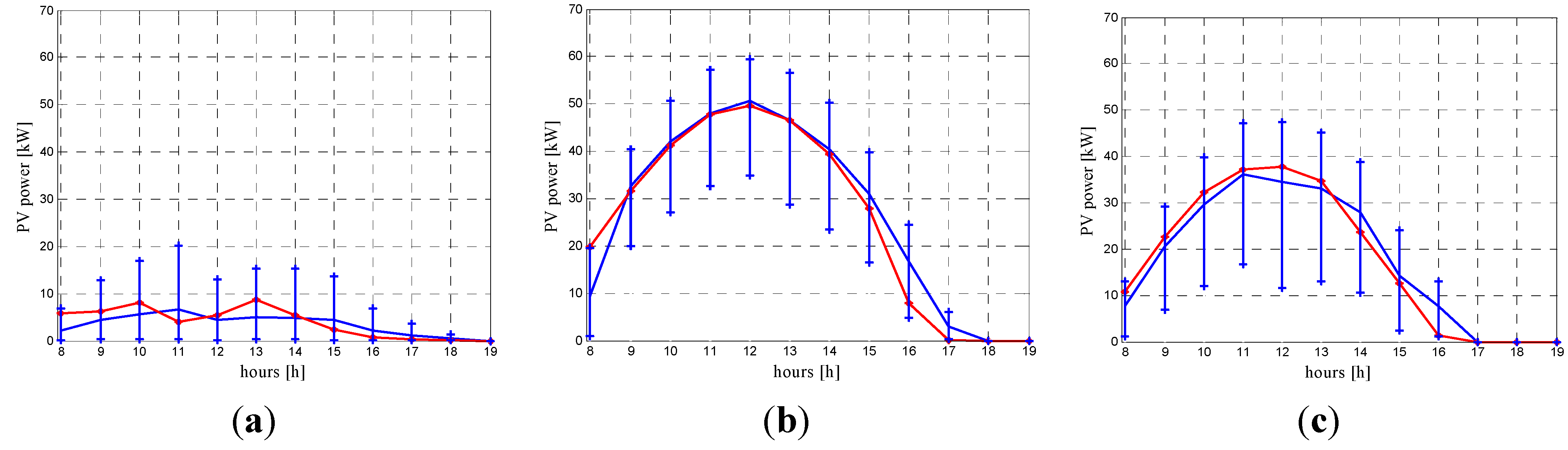
4. Experimental Section

In this section, the proposed Bayesian forecasting method is applied to a 75-kWp PV system, presenting an array surface ${\mathrm{S}}_{\mathrm{C}}=600$ m² and an efficiency $\mathsf{\eta }=0.09$. Measurements of the clearness indexand of the meteorological variables cited in the Subsection 3.4 (air temperature, relative humidity, wind speed and total cloud cover) are available at the website of the National Renewable Energy Laboratory. In particular, a meteorological station in Colorado (39.742° N, 105.18° W) has been selected and measurements referred to the time interval [8 a.m., 8 p.m.] and collected every 15 minutes are chosen.

In the following, at first a correlation analysis is performed to individuate the meteorological variables to be included in the time series AR model; then, the proposed method is used to forecast the pdf of the hourly active power produced by the PV system.

To individuate the most suitable AR time series model, an “off-line” correlation analysis between the clearness index and the meteorological variables is carried out, on the basis of measurements recorded from January to December 2010. Figure 2 reports the time evolution of the correlation coefficient between the clearness index and the meteorological variables. To avoid excessive computational efforts, only the meteorological variables furnishing the highest values of the correlation coefficient are taken into account. As such, the analysis of the Figure 2 clearly reveals that the total cloud cover and the relative humidity are the meteorological variables presenting the highest influence on the clearness index; consequently, the AR time-series model in Equation (12) reduces to:

$${\mu }_{K_{h+1}}= {\alpha }_1{k}_h+{\beta }_{1}r{h}_h+{\beta }_{2}c{c}_h+{\alpha }_0$$

(19)

To make inference about the prior random parameters ${\mathsf{\alpha }}_0,{\mathsf{\alpha }}_1$, ${\mathsf{\beta }}_1$ and ${\mathsf{\beta }}_2$, the sets ${\mathit{S}}_{{\mathit{K}}_{\mathit{h}}}, {\mathit{S}}_{\mathit{C}{\mathit{C}}_{\mathit{h}}}, {\mathit{S}}_{\mathit{R}{\mathit{H}}_{\mathit{h}}}$ (see Subsection 3.4) contain $N_h=144$ measurements collected at time intervals of 15 minutes recorded before the hour $h$ of the forecast.

Figure 2. Time evolution of the correlation coefficient between the clearness index and the selected meteorological variables.

Figure 2. Time evolution of the correlation coefficient between the clearness index and the selected meteorological variables.

The application of the proposed approach to forecast the hourly PV active power is performed referring to the four seasons of the 2011. Figure 3, Figure 4, Figure 5 and Figure 6 show, respectively, the actual measured values of the PV active powers (red lines), the mean value (blue line) and the range between the 5th and 95th percentile values of the forecasted pdfs of hourly PV active power. In particular, the results refer to the Recommended Average days of winter (Figure 3), spring (Figure 4), summer (Figure 5) and autumn (Figure 6). In [22] Recommended Average Days are days which have the extraterrestrial radiation closest to the average value in the month. A similar behavior characterizes the vast majority of the considered days (in almost all considered days).

Figure 3. Actual measures of the hourly PV active power (red line); mean values (blue line) and range between 5th and 95th percentile values of the forecasted pdfs of the hourly PV active power. (a) 17 January; (b) 16 February; and (c) 10 December.

Figure 3. Actual measures of the hourly PV active power (red line); mean values (blue line) and range between 5th and 95th percentile values of the forecasted pdfs of the hourly PV active power. (a) 17 January; (b) 16 February; and (c) 10 December.

Figure 4. Actual measures of the hourly PV active power (red line); mean values (blue line) and range between 5th and 95th percentile values of the forecasted pdfs of the hourly PV active power. (a) 16 March; (b) 15 April; and (c) 15 May.

Figure 4. Actual measures of the hourly PV active power (red line); mean values (blue line) and range between 5th and 95th percentile values of the forecasted pdfs of the hourly PV active power. (a) 16 March; (b) 15 April; and (c) 15 May.

Figure 5. Actual measures of the hourly PV active power (red line); mean values (blue line) and range between 5th and 95th percentile values of the forecasted pdfs of the hourly PV active power. (a) 11 June; (b) 17 July and; (c) 16 August.

Figure 5. Actual measures of the hourly PV active power (red line); mean values (blue line) and range between 5th and 95th percentile values of the forecasted pdfs of the hourly PV active power. (a) 11 June; (b) 17 July and; (c) 16 August.

Figure 6. Actual measures of the hourly PV active power (red line); mean values (blue line) and range between 5th and 95th percentile values of the forecasted pdfs of the hourly PV active power. (a) 15 September; (b) 15 October and; (c) 14 November.

Figure 6. Actual measures of the hourly PV active power (red line); mean values (blue line) and range between 5th and 95th percentile values of the forecasted pdfs of the hourly PV active power. (a) 15 September; (b) 15 October and; (c) 14 November.

From the analysis of the figures, it appears that the actual values of the hourly PV active power are always comprised between the 5th and 95th percentile values. In addition, it should be noted that the mean value appears in most cases a good estimator for the forecasted pdfs, particularly in the range of hours between 11 a.m. and 3 p.m. At the beginning (end) of the period characterized by the presence of solar radiation, usually higher (lower) percentiles appear the most adequate estimators. Anyway, if the mean value of forecasted pdf would be used as the only estimator of the forecasted PV power, the Mean Absolute Relative Error (MARE), defined as:

$$MARE=\frac{1}{N}{\displaystyle \sum }_{h=1}^N\frac{\left|P_{P{V}_h}-P_{P{V}_h}^{*}\right|}{P_{P{V}_h}}$$

(20)

is estimated between 14.5% (winter season) and 18.0% (autumn season).

Finally, Figure 7 and Figure 8 show the forecasted (represented by a blue histogram) and the analytical (represented by a continuous red line) pdfs of the hourly PV active power in March (Figure 7a), April (Figure 7b), August (Figure 8a) and September (Figure 8b). The analytical pdf is obtained applying the fundamental theorem for the function of a random variable to Equation (9) proposed in [31]. From the analysis of Figure 7 and Figure 8 it is evident that in different conditions of solar radiation the forecasted pdfs are close to the analytical distributions.

Figure 7. Forecasted (histogram) and analytical (red line) pdfs of PV power. (a) h = 1 p.m. of 16 March; and (b) h = 11 a.m. of 15 April.

Figure 7. Forecasted (histogram) and analytical (red line) pdfs of PV power. (a) h = 1 p.m. of 16 March; and (b) h = 11 a.m. of 15 April.

Figure 8. Forecasted (histogram) and analytical (red line) pdfs of PV power. (a) h = 2 p.m. of 16 August and; (b) h = 1 p.m. of 15 September.

Figure 8. Forecasted (histogram) and analytical (red line) pdfs of PV power. (a) h = 2 p.m. of 16 August and; (b) h = 1 p.m. of 15 September.

5. Conclusions

A new method based on the Bayesian inference has been proposed to perform a short-term forecasting of the active power produced by a photovoltaic system starting from an estimation of the hourly clearness index. It takes into account the dependence of the terrestrial solar radiation on some explanatory atmospheric variables, including the cloud cover and humidity. The combination of probabilistic techniques, such as Bayesian inference and Monte Carlo simulation, allows to provide the predictive probability density function of the photovoltaic generated power, which is very useful for the optimal operation and control of the smart grids of the future.

However, if only a value is requested as estimator of the forecasted photovoltaic power, arises the problem of individuate which pdf parameter (mean value, percentiles ...) is the most representative for the distribution. Moreover, the non-linear relationship between the clearness index and the photovoltaic power output can reflect in not negligible errors in the forecasted distributions of the photovoltaic power. Then, future works will investigate the direct application of the proposed probabilistic forecasting method to the active power produced by the PV system, even if the application of the Bayesian inference in this case seems to be arduous. The research will also focus on the choice of the best parameter to be extracted from the predicted probability distribution so as to test the performance of the proposed method in terms of traditional measures of the forecasting accuracy; in this case comparison with ARIMA and neural networks methods will be affected.

References

1. Bouhafs, F.; Mackay, M.; Merabti, M. Links to the future: Communication requirements and challenges in the smart grid. IEEE Power Energy Mag. 2012, 10, 24–28. [Google Scholar] [CrossRef]
2. Pilo, F.; Pisano, G.; Soma, G.G. Optimal coordination of Energy resources with a two-stage online active management. IEEE Trans. Ind. Electron. 2011, 58, 4526–4537. [Google Scholar] [CrossRef]
3. Potter, C.M.; Archambault, A.; Kenneth, W. Building a smarter smart grid to better renewable energy information. In Proceedings of Power Systems Conference and Exposition (PSCE 09), Seattle, WA, USA, 15–18 March 2009.
4. Smith, J.C.; Milligan, M.R.; De Meo, E.A.; Parson, B. Utility wind integration and operating impact state of art. IEEE Trans. Power Syst. 2007, 22, 900–907. [Google Scholar] [CrossRef]
5. Pinson, P.; Chevallier, C.; Kariniotakis, G.N. Trading wind generation from short-term probabilistic forecasts of wind power. IEEE Trans. Power Syst. 2007, 22, 1148–1156. [Google Scholar] [CrossRef]
6. Sharma, N.; Sharma, P.; Irwin, D.; Shenoy, P. Predicting solar generation from weather forecast using machine learning. In Proceedings of IEEE International Conference on Smart Grid Communications (SmartGridComm), Bruxelles, Belgium, 17–20 October 2011; pp. 528–533.
7. Watson, R. IEA Expert Meeting on Wind Forecasting Techniques; NREL Report; NREL (National Renewable Energy Laboratory): Golden, CO, USA, 2000. [Google Scholar]
8. Liserre, M.; Sauter, T.; Hung, J.Y. Future energy systems: Integrating renewable energy sources into the smart power grid through industrial electronics. IEEE Ind. Electron. Mag. 2010, 4, 18–37. [Google Scholar] [CrossRef]
9. Mellit, A.; Massi Pavan, A. A 24-h forecast of solar irradiance using artificial neural network: Application for performance prediction of a grid-connected PV plant at Trieste, Italy. Sol. Energy 2010, 84, 807–821. [Google Scholar]
10. Al Riza, D.F; Gilani, S.I.; Aris, M.S. Hourly solar radiation estimation using ambient temperature and relative humidity data. Int. J. Environ. Sci. Dev. 2011, 2, 188–193. [Google Scholar] [CrossRef]
11. Yona, A.; Senjyu, T.; Funabashi, T. Application of recurrent neural network to short-term-ahead generating power forecasting for photovoltaic system. In Proceedings of IEEE Power Engineering Society General Meeting, Tampa, FL, USA, 24–28 June 2007.
12. Lorenz, E.; Hurka, J.; Heinemann, D.; Beyer, H.G. Irradiance forecasting for the power prediction of grid-connected photovoltaic systems. IEEE J. Sel. Top. Appl. Earth Obs. Remote Sens. 2009, 2, 2–10. [Google Scholar] [CrossRef]
13. Li, Y.; He, L.; Nie, R. Short-term forecast of power generation for grid-connected photovoltaic system based on advanced Grey-Markov chain. In Proceedings of IEEE International Conference on Energy and Environment Technology (ICEET ’09), Guilin, China, 16–18 October 2009; Volume 2, pp. 275–278.
14. Bacher, P.; Madsen, H.; Nielsen, P. Online short-term solar power forecasting. Sol. Energy 2009, 83, 1772–1783. [Google Scholar] [CrossRef]
15. Hassanzadeh, M.; Etezadi-Amoli, M.; Fadali, M.S. Practical approach for sub-hourly and hourly prediction of PV power output. In Proceedings of IEEE Conferences North American Power Symposium, Arlington, TX, USA, 1–5 September 2010.
16. Bracale, A.; Caramia, P.; Fantauzzi, M.; Di Fazio, A.R. A Bayesian-based approach for photovoltaic power forecast. In Proceedings of Cigrè International Symposium on Smart Grid, Bologna, Italy, 13–15 September 2011.
17. Bracale, A.; Caramia, P.; De Martinis, U.; Di Fazio, A.R. An improved Bayesian-based approach for short term photovoltaic power forecasting in smart grids. In Proceedings of International Conference on Renewable Energies and Power Quality (ICREPQ 2012), Santiago De Compostela, Spain, 28–30 March 2012.
18. Bracale, A.; Caramia, P.; Carpinelli, G.; Di Fazio, A.R.; Varilone, P. A Bayesian-based approach for very short-term steady-state analysis of a smart grid. IEEE Trans. Smart Grids 2013, in press. [Google Scholar]
19. Gelman, A.; Carlin, J.B.; Stern, H.S.; Rubin, D.B. Bayesian Data Analysis; Chaoman & Hall: London, UK, 1995. [Google Scholar]
20. Papoulis, A. Probability, Random Variables and Stochastic Processes; McGraw-Hill: New York, NY, USA, 1991. [Google Scholar]
21. Zhang, J.; Pu, J.; McCalley, J.D.; Stern, H.; Gallus, W.A., Jr. A Bayesian approach to short term transmission line thermal overload risk assessment. IEEE Trans. Power Deliv. 2002, 17, 770–778. [Google Scholar] [CrossRef]
22. Duffie, J.A.; Beckman, W.A. Solar Engineering of Thermal Processes, 2nd ed.; Wiley Interscience: New York, NY, USA, 1991. [Google Scholar]
23. Orgill, J.F; Hollands, K.T.G. Correlation equation for hourly diffuse radiation on a horizontal surface. Sol. Energy 1977, 19, 357–359. [Google Scholar] [CrossRef]
24. Kroposki, B.; Emery, K.; Myers, D.; Mrig, L. A comparison of photovoltaic module performance evaluation methodologies for energy ratings. In Proceedings of First World Conference on Photovoltaic Energy Conversion (WPEC 1994), Hawaii, HI, USA, 5–9 December1994; pp. 858–862.
25. Ettoumi, F.Y.; Mefti, A.; Adane, A.; Bouroubi, M.Y. Statistical analysis of solar measurements in Algeria using beta distributions. Renew. Energy 2002, 124, 28–33. [Google Scholar]
26. Ibanez, M.; Beckman, W.A.; Sanford, A.K. Frequency distributions for hourly and daily clearness indices. J. Sol. Energy Eng. 2002, 26, 47–67. [Google Scholar]
27. Liu, B.Y.H.; Jordan, B.C. The interrelationship and characteristic distribution of direct, diffuse and total solar radiation. Sol. Energy 1960, 4, 1–19. [Google Scholar] [CrossRef]
28. Bendt, P.; Collares-Pereira, M.; Rabl, A. The frequency distribution of daily insolation values. Sol. Energy 1981, 27, 1–19. [Google Scholar] [CrossRef]
29. Hollands, K.T.G.; Huget, R.G. A probability density function for clearness index, with applications. Sol. Energy 1983, 30, 195–209. [Google Scholar] [CrossRef]
30. Huang, Y.; Lu, J.; Liu, C.; Xu, X.; Wang, W.; Zhou, X. Comparative study of power forecasting methods for PV stations. In Proceedings of International Conference on Power System Technology (POWERCON 2010), Hangzhou, China, 24–28 October 2010; pp. 1–6.
31. Conti, S.; Raiti, S. Probabilistic load flow using Monte Carlo techniques for distribution networks with photovoltaic generators. Sol. Energy 2007, 81, 1473–1481. [Google Scholar] [CrossRef]