1. Introduction
The growing requirements for electricity and the pollution caused by burning fossil fuels has led to a renaissance of nuclear energy industry, even if there have been some severe accidents such as Three Mile Island (USA), Chernobyl (Ukraine) and Fukushima (Japan). Since power-level control is a quite crucial technique which guarantees operation stability and efficiency for nuclear reactors, developing high performance power-level regulators is quite meaningful for the current rebirth of nuclear energy industry. Compared with the classical static output feedback power-level control laws, the advanced power regulation strategies have the potential of strengthening both the closed-loop stability and control performance by feeding back the internal system state-variables. Due to the absence of adequate sensors, some state-variables associated with the dynamics of a nuclear reactor are not available for measurement. In order to implement the advanced power-level control strategies for stronger dynamic performance, some observation structure should be used to reconstruct the state-variables that cannot be obtained directly through measurement. In this case, the simpler solution is to utilize the linear observers such as the Luenberger observer [
1] and Kalman filter [
2,
3]. However, the dynamic behavior of a given nuclear reactor exhibits strong nonlinearity and it depends on many factors such as power-level, fuel burnup,
etc. The linear observers can only provide satisfactory performance in a small neighborhood near an operating point. Thus, if large variations of the system state variables are required, especially in the case of load following, the previous option is not effective anymore, and nonlinear observers should be developed. Shtessel gave a sliding mode observer to construct a dynamic output feedback loop with a static state-feedback sliding mode controller for regulating the power-level of space nuclear reactor TOPAZ II [
4]. Etchepareborda applied the high gain observer to design a nonlinear model predictive power-level control for a pressurized water reactor (PWR)-like research reactor [
5]. Dong proposed the dissipation-based high gain filter (DHGF) for the state-observation of PWRs [
6], and then applied the DHGF to build the dynamic output-feedback power-level control laws [
7,
8]. However, the precondition of applying these nonlinear observers is to know the accurate lump-parameter dynamic model of a given nuclear reactor. Although some schemes have been introduced to strengthen the adaptation performance of nonlinear observers to system uncertainties, there are strong constraints on the form of system uncertainties [
9]. Therefore, more advanced schemes should be given to further improve the adaptability of nonlinear observation.
Artificial neural networks (ANNs), inspired by biological neural networks, are composed of simple processing elements called neurons normally arranged in layers and interconnected to each other by some weighted connections. This architecture along with a learning algorithm for adjusting the connection weights, exhibits some interesting properties such as learning, approximation and parallel distributed processing capability. The radial basis function (RBF) network and multi-layer perceptron (MLP) network are two widely utilized ANNs. It has been proven theoretically that both the RBF [
10,
11] and MLP [
12,
13,
14] networks can approximate a wide range of nonlinear functions to any desired degree of accuracy under certain conditions. In recent years, ANNs have also been applied to nuclear engineering, particularly, for reactor control. Ku, Lee and Edwards applied the diagonal recurrent neural network (DRNN) to a nuclear reactor model to improve its temperature response, and here the DRNNs must be trained offline by a linearized reactor model and a pre-designed optimal temperature control [
15]. Arab-Alibeik and Setayeshi designed a neural adaptive inverse controller for regulating the power-level of a PWR, and here the ANN was also trained offline by a reactor model [
16]. From the above works in applying ANN in nuclear engineering, it was shown that the identification must be sufficiently accurate before control action is initiated. However, in practical control applications, it is desirable to have systematic method of ensuring the stability and robustness of the overall system. In the past few years, several ANN-based control laws for nonlinear systems have been proposed based upon Lyapunov stability theory. One main advantage of these schemes is that the adaptive laws were derived based on the Lyapunov synthesis method and thus can provide the closed-loop stability. Ge
et al. proposed an adaptive state-feedback control law for a large class of nonlinear systems based on the RBF network, and the regulating error was proved to converge to a small neighborhood of the origin by using Lyapunov stability theory [
17]. Moreover, state-feedback control design methods based on the MLP network were also studied for nonlinear systems in Brunovksy, pure-feedback and lower-triangular forms by using Lyapunov stability theory and techniques of feedback linearization and backstepping [
18,
19,
20,
21,
22]. It is clear that designing a satisfactory state-observer is the precondition of implementing advanced state-feedback control laws. Since there usually exist system dynamics uncertainties the adaptive observer design method based upon ANNs is another hot topic nowadays. Vargas and Hemerly proposed an adaptive observer for unknown general nonlinear systems based upon both RBF networks and Lyapunov stability theory, and the adaption laws of the weights provide the bounded-error performance [
23]. By the use of the adaptive bounding technique, Stepanyan and Hovakimyan gave a RBF-based adaptive observer which could provide asymptotically convergent state estimation for a class of uncertain nonlinear systems [
24]. Very recently, Yang
et al. also designed a stable RBF-based observer to build a model referenced adaptive controller (MRAC) for an electrohydraulic system [
25]. Since the MLP network is nonlinear in its parameters and can be applied to many systems with arbitrary degrees of nonlinearity and complexity, it has already been used to design adaptive observers. Abdollahi
et al. gave an MLP-based observer for nonlinear systems by Lyapunov direct method, and then applied it to the state-estimation of flexible-joint manipulators [
26]. Pérez-Cruz and Poznyak gave a stable observer for estimating the precursor power and internal reactivity of a nuclear reactor by combining the MLP network and sliding mode technique [
27]. Talebi
et al. designed a recurrent neural-network-based state-observer for sensor and actuator fault detection of the satellite’s attitude control subsystem [
28].
Since a nuclear fission reactor is by nature a complex nonlinear system with its parameters varying with time as a function of power-level, fuel burnup, xenon isotope production, control rod worth, etc., it is very necessary to design nonlinear observers for nuclear reactors with the adaptability to those parameter uncertainties. In this paper, a nonlinear adaptive observer is developed to PWRs by the use of MLP network. Based upon Lyapunov stability theory, both the boundness and convergence property of the observation error is first proved. Then, this observer is applied to the state-observation of a nuclear heating reactor (NHR) which is a special type of PWR with some properties such as natural circulation and self-pressurization. Numerical simulation results not only verify the feasibility of this newly-built observer but also show the relationship between its parameters and performance.
3. Observer Design
It is clear that solving Problem 1 is equivalent to giving the tuning approach for both feedback gains KO and kOξ and weighting matrices and of MLP. In this section, this tuning approach, which provides bounded and convergent observation, will be given based on Lyapunov stability theory. Before giving the main result of this paper, a useful lemma is firstly introduced as follows.
Lemma 1. The approximation error of
MLP to
GMLP defined by:
satisfies:
where:
and
dr is the residual term. Moreover,
dr satisfies:
where
ci (
i = 0,1,2,3) are certain positive scalars.
Proof: It is easy to see that the Taylor expansion of
S(
VTx) about
can be written as:
where:
and
denotes the sum of the high order terms in the Taylor series expansion. Based on Equation (30), we can derive that:
where:
and:
Then, we can clearly see from Equation (32) that Equation (25) is well satisfied.
Moreover, since we have assumed that activation function
s takes the form as Equation (13), it is clear that:
and we can also derive that:
From Equation (38), it is easy to check that for
:
and:
Based on Inequalities (39) and (40), we have:
and:
Moreover, from Taylor expansion Equation (30), we can know that:
Then, based on Assumption (17) and Inequalities (37) and (41)–(43), we have:
By Equation (33), it can be seen that:
We can see that Inequality (29) certainly holds. This completes the proof of Lemma 1.
Remark 1. From Lemma 1, the norm of residual term dr is influenced by the norms of systems state x, observation error e and approximation error of weighting matrix .
The following Theorem 1, which is the main result of this paper, proposes the design of nonlinear adaptive state-observer based on the MLP neural network.
Theorem 1. Consider state observer Equation (21) of PWR dynamics Equation (7), and suppose that observer gains
kOξ is positive and system state-vector
x is bounded. Let observer gain matrix
KO take the form as:
where observer gains
kON,
kOF and
kOC are all positive. Furthermore, choose the learning algorithms of weighting matrices
and
of multilayer network
MNN as:
and:
respectively, where both
ΓW and
ΓV are diagonal positive-definite matrices, both scalars δ
W and δ
V are positive:
δ is a positive scalar and matrix
C is defined by Equation (20). Then observation errors
e and
eξ defined by:
and:
are convergent and bounded.
Proof: From Equations (7), (21), (47), (53) and (54), the dynamics of observation error
e satisfies:
where:
and approximation error
de is defined by Equation (14).
Moreover, from Equations (19) and (22):
from which we have:
Choose the Lyapunov function of the observation error dynamics Equation (55) as:
where:
Differentiate
Ve1 along the trajectory given by Equation (55):
where matrix
Σ given by Equation (50) is still a diagonal and positive-definite.
Moreover, from Equation (59), we can derive that:
Further, since:
and:
from Equation (63), we have:
Substitute Inequality (66) to Equation (62):
where:
and:
Then, differentiate
Ve along the trajectory given by observation error dynamics Equation (55):
From Inequality (72), if we choose the learning algorithms of the weighting matrices as Equations (48) and (49), then it is clear that:
where:
and:
Here, scalars δW and δV should be chosen so that both υW and υV are positive.
Based on the assumption about the boundness of system state x and Inequalities (15)–(17) and (29), it is clear from Inequality (73) that the observation errors e and eξ are convergent and bounded. This completes the proof of Theorem 1.
Remark 2. The MLP-based nonlinear adaptive observer determined by Equations (21) and (47)–(49) does not need any matching condition of system uncertainty
σ. However, the existing adaptive observers for nuclear reactors such as the observer presented in [
9] still needs some matching condition on the system uncertainty. This means that the neural observer given in this paper is able to deal with general bounded system uncertainties, which is the key advanced feature of this novel neural observer design technique. Moreover, from Equations (21), (48) and (49),
,
and
are updated simultaneously. If the perceptron number of the hidden layer is not large, the simultaneous updating of state-estimation
and weighting matrices
and
cannot affect the real-time performance of the algorithm.
4. Simulation Results with Discussions
To verify the feasibility of this newly-built neural observer, it is applied to the state-observation of a NHR which is a small PWR developed by Institute of Nuclear and New Energy Technology (INET) at Tsinghua University in this section. The NHR has many advanced safety features such as integrated arrangement, natural circulation at any power-levels, self-pressurization, hydraulic control rod driving, and passive residual heat removing [
30,
31,
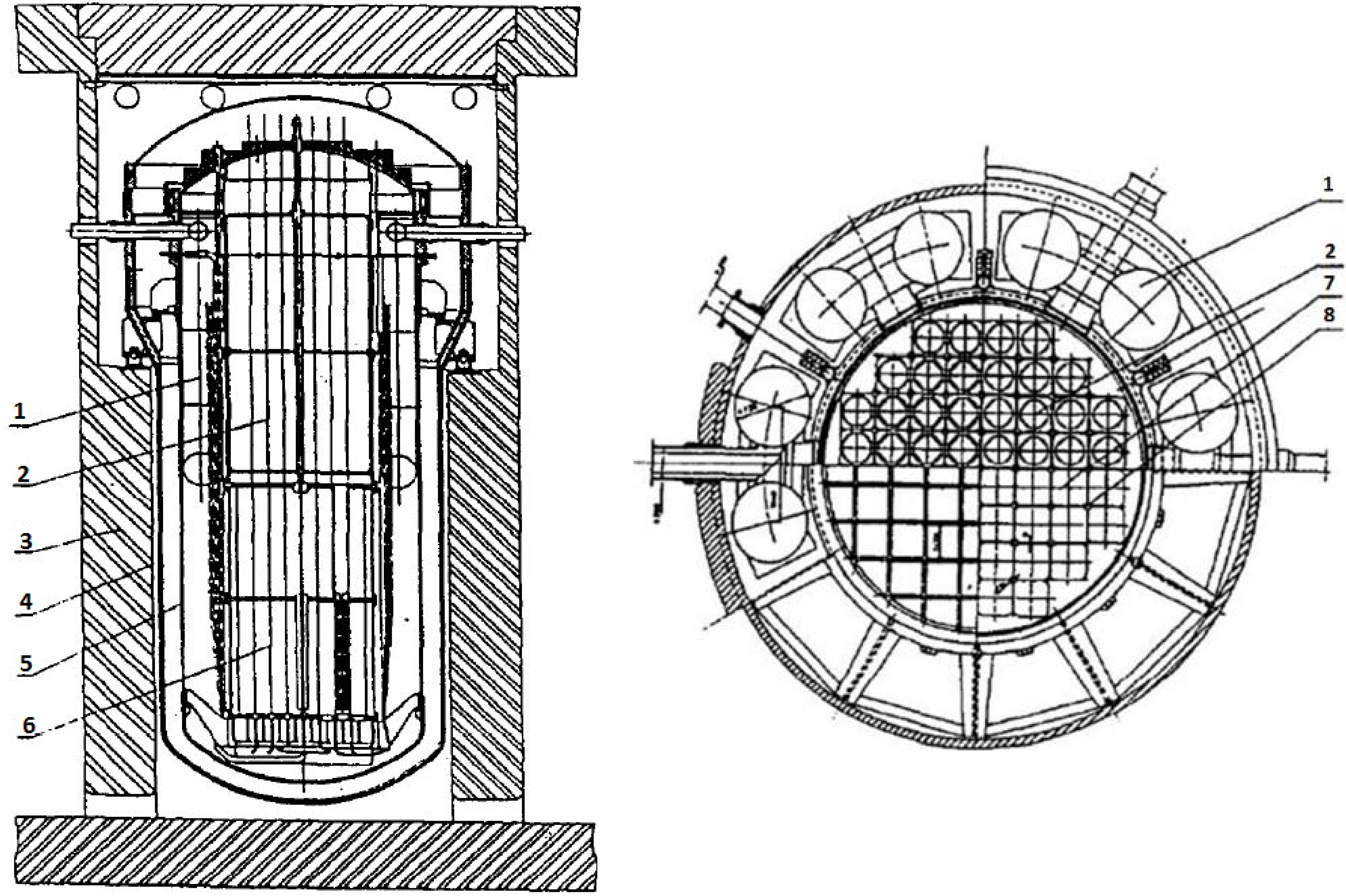
32], and it can be applied to the fields such as district heating, seawater desalination and electricity production. The structure of the NHR is illustrated in
Figure 1. Since NHR dynamics has both strong nonlinearity and high uncertainty, in order to implement advanced power-level controllers for higher operation performance, it is very meaningful to realize the adaptive state-observation for the NHR.
Figure 1.
Structure and cross section of the NHR: (1) Primary heating exchanger; (2) Riser; (3) Biological shield; (4) Containment; (5) Pressure vessel; (6) Core; (7) Fuel elements and (8) Control rods.
Figure 1.
Structure and cross section of the NHR: (1) Primary heating exchanger; (2) Riser; (3) Biological shield; (4) Containment; (5) Pressure vessel; (6) Core; (7) Fuel elements and (8) Control rods.
4.1. Description of the Numerical Simulation
The simulation model of the NHR is composed of the point kinetics model with six delayed neutron groups and lumped dynamic model of the reactor thermal-hydraulics, primary heat exchanger, U-tube steam generator (UTSG), feedwater pump of the UTSG and necessary pipe or volume cells [
33]. The parameters of the NHR at the middle of the fuel cycle in 100% power-level are shown in
Table 1. The output-feedback-dissipation power-level control strategy given in [
34] is adopted here. Moreover, in this simulation, we choose
l = 4,
kON =
kOC = 0.0001,
kOF = 10.0,
kOξ = 1.0:
where both δ
wv and
rp are given positive scalars. The initial values of interconnection matrices
and
,
i.e.,
and
are set to be
and
, respectively.
Table 1.
NHR Parameters at the Middle of the Fuel Cycle in 100% Power-Level.
Table 1.
NHR Parameters at the Middle of the Fuel Cycle in 100% Power-Level.
| Symbol | Quantity | Symbol | Quantity |
|---|
| β | 0.0069 | αf | −2.48 × 10⁻⁵ (1/°C) |
| Λ | 4.18 × 10⁻⁵ (s) | αc | −2.71 × 10⁻⁴ (1/°C) |
| λ | 0.08 (1/s) | M | 4.29 (kW/°C) |
| μf | 5.01 (MWs/°C) | Ω | 1.06 (MW/°C) |
| μc | 69.23 (MWs/°C) | P0 | 200 (MW) |
Case A (large load increase): The load signal changes linearly from 20% to 100% in a minute.
δwv = 0.01, and different rp is adopted in the simulation.
rp = 1.0, and different δwv is adopted.
Case B (large load decrease): The power demand decreases linearly from 100% to 20% in a minute.
δwv = 0.01, and different rp is adopted in the simulation.
rp = 1.0, and different δwv is adopted.
4.2. Simulation Results
In this numerical simulation, the following two case studies are done to show the state-observing performance of MNN-based nonlinear adaptive observer determined by Equations (21) and (47)–(49).
4.2.1. Large Load Increase
This verification represents a hard operation for the NHR. In this case, the power demand increases linearly from 20% to 100% in 60 s.
The observation errors of variations of the relative nuclear power, the relative precursor concentration, and the average temperatures of the fuel and coolant,
i.e., the observation errors of state-variables δ
nr, δ
cr, δ
Tf and δ
Tcav with constant δ
wv and different
rp are all illustrated in
Figure 2. Furthermore, the observation errors of these state-variables with different δ
wv and constant
rp are shown in
Figure 3.
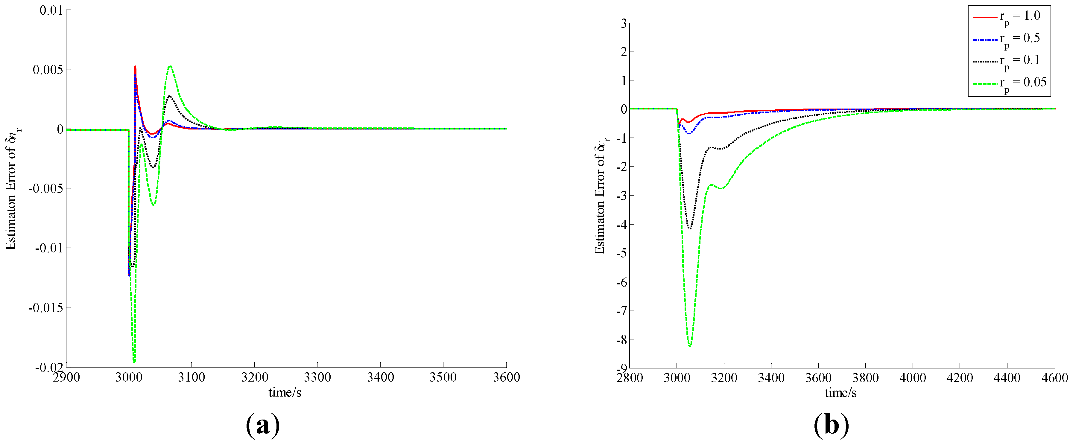
Figure 2.
Observation errors of (a) δnr; (b) δcr; (c) δTf and (d) δTcav in case of A1.
Figure 2.
Observation errors of (a) δnr; (b) δcr; (c) δTf and (d) δTcav in case of A1.
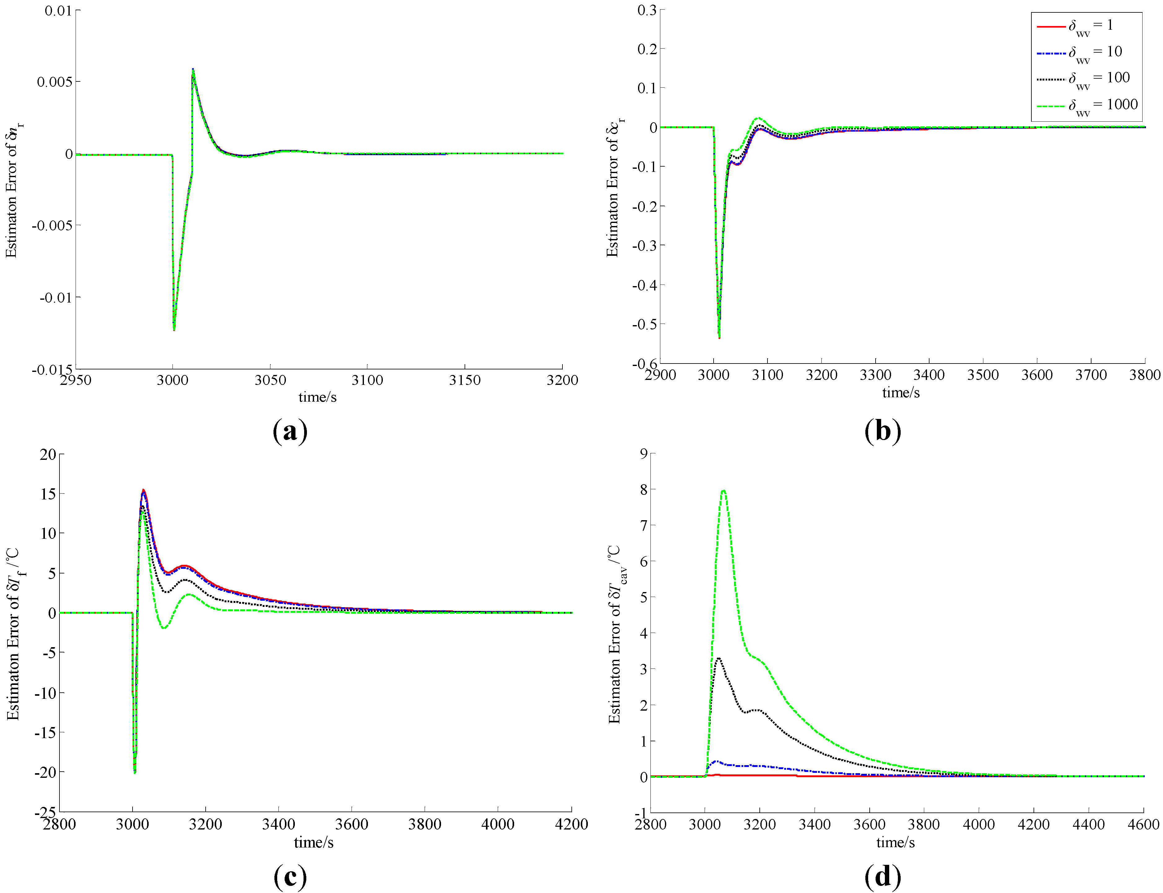
Figure 3.
Observation errors of (a) δnr; (b) δcr; (c) δTf and (d) δTcav in case of A2.
Figure 3.
Observation errors of (a) δnr; (b) δcr; (c) δTf and (d) δTcav in case of A2.
4.2.2. Large Load Decrease
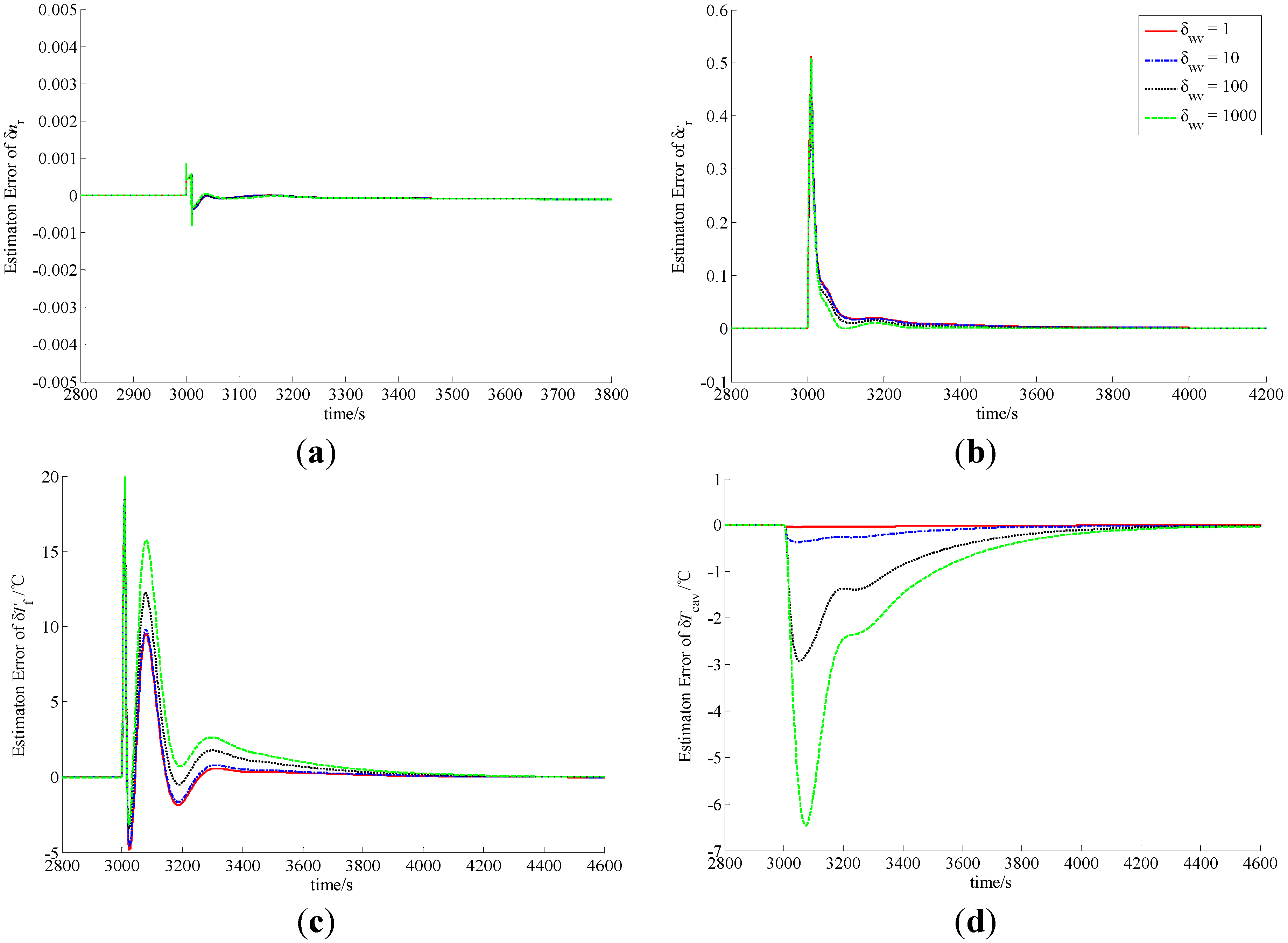
This case also represents a stressed operation for the NHR. The load signal changes linearly from 100% to 20% in a minute. The observation errors of state-variables δ
nr, δ
cr, δ
Tf and δ
Tcav with constant δ
wv and different
rp are all shown in
Figure 4, and the responses of these observation errors with different δ
wv and constant
rp are given in
Figure 5.
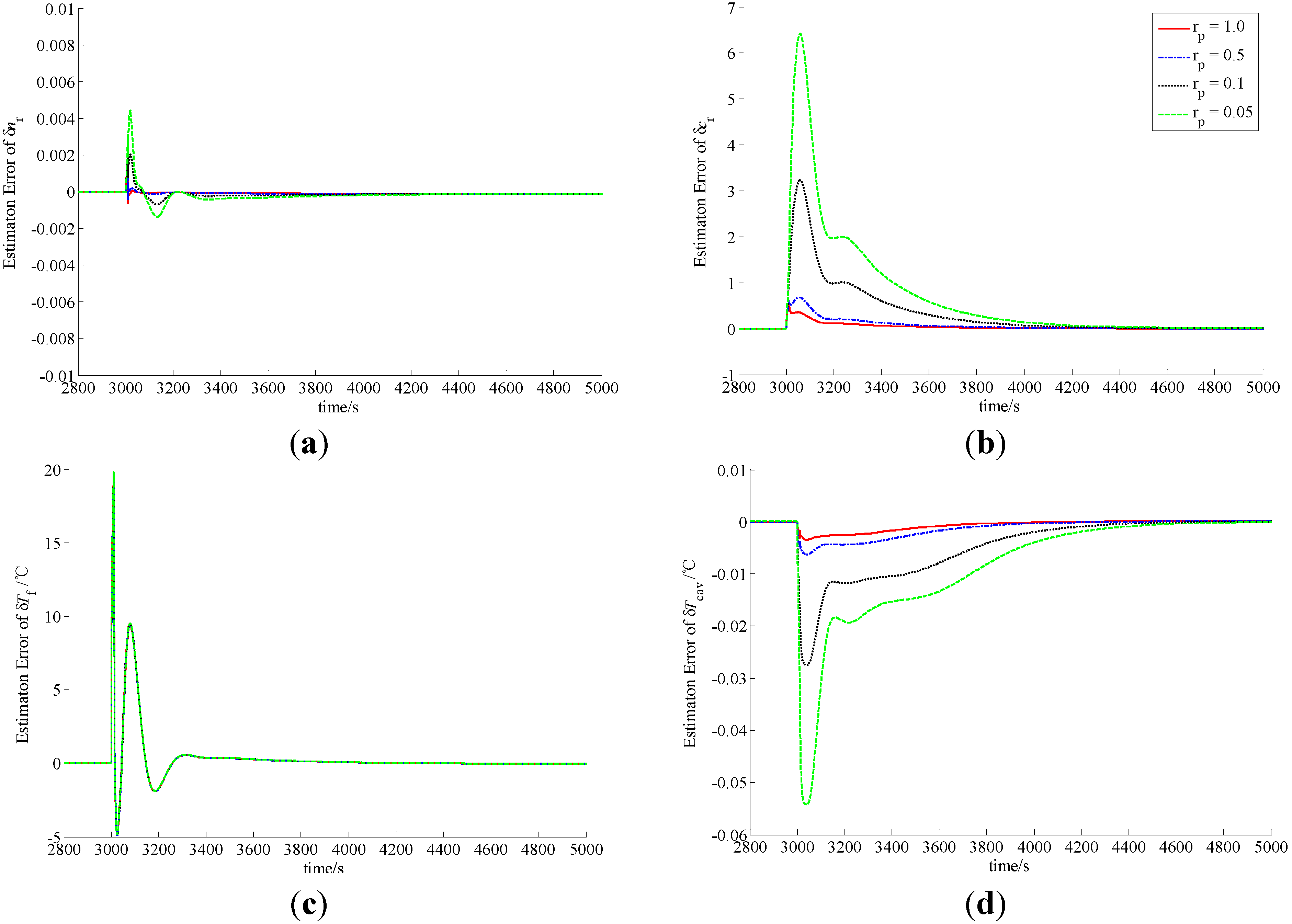
Figure 4.
Observation errors of (a) δnr; (b) δcr; (c) δTf and (d) δTcav in case of B1.
Figure 4.
Observation errors of (a) δnr; (b) δcr; (c) δTf and (d) δTcav in case of B1.
Figure 5.
Observation errors of (a) δnr; (b) δcr; (c) δTf and (d) δTcav in case of B2.
Figure 5.
Observation errors of (a) δnr; (b) δcr; (c) δTf and (d) δTcav in case of B2.
4.3. Discussion
In the procedure of load lift, the load increases rapidly from 20% to 100% in 60 s. Since the actual power level cannot vary so quickly, δnr becomes smaller, which indicates that the actual power level of the NHR is smaller than the load set by the operator in the initial phase of the process. Due to the function of power level controller, δnr becomes larger and larger, and finally equals zero. The difference of the power level causes the variations of the precursor concentration and average temperatures of the fuel and coolant inside the reactor core. Similarly, in the case of a load decrease from 100% to 20% in a minute, the actual power level also cannot change so fast, and therefore δnr become larger, which indicates that the actual power level of the NHR is higher than the load in the initial stage. Then the power-level becomes lower and lower due to the function of power controller, and finally reaches the full power-level.
From
Figure 2,
Figure 3,
Figure 4 and
Figure 5, the MLP-based state-observer developed in this paper can provide bounded and convergent state-observations. The load variation leads to the variation of the state variables, which causes the variation of system output. The variation of system output then drives both the observer and learning algorithms of the MLP connection weights to generate a convergent state-observation. It is also clear from these figures that the variation of observer parameters cannot change the boundness and convergence of the state-observation. Further, from
Figure 2 and
Figure 4, if positive scalar
rp is larger, then the observation performance is higher. Actually, from Equation (79), scalar
rp is larger, the influence of
eO to the weighting connections that correspond to the state-observation of the thermal-hydraulic loop is stronger, which leads to higher observation performance of δ
Tcav. From both Equations (55) and (57), since
e4,
i.e., the observation error of δ
Tcav can affect the state-observation of neutron kinetics, higher observation performance of δ
Tcav is positive to improve the observation quality of neutron kinetics. Moreover, from
Figure 3 and
Figure 5, it is easy to see that if positive scalar δ
wv is larger, the observation performance of δ
Tcav is worse. However, there is a little improvement to the observation performance of δ
cr and δ
Tf. Based upon the above discussion, MLP-based nonlinear state-observer composed of Equations (21), (47)–(49) provides both bounded and convergent observation of system state-variables, and the parameters of this observer should be properly adjusted.
From the curves plotted in
Figure 2,
Figure 3,
Figure 4 and
Figure 5, both the overshoots and settling periods of the estimation errors of unmeasurable state δ
cr and δ
Tf can be reduced to acceptable limits with properly selected scalars
rp and δ
wv, which leads to practical feasibility of this newly-built observer. Usually,
rp should be larger, and δ
wv should be selected based upon the trade-off between the observation performance of δ
Tcav and that of δ
cr and δ
Tf. Moreover, with comparison to the sliding mode observer [
4], high gain observer [
5] and DHGF [
6], the main virtue of MLP-based nonlinear observer proposed in this paper is its high adaptation capability to system uncertainties. That is to say that this new observer has the adaptation performance that other observers for nuclear reactors do not have.
Finally, due to the widely utilization of those advanced digital control system platforms, there is no difficulty in realizing the MLP-based observer presented in this paper. Furthermore, since there have been some mature MLP network programs, it is easy for the engineers to implement both observer Equation (21) and learning Algorithms (48) and (49) as a software running on a digital platform.


