1. Introduction
Recently, the popularity of PV power generation systems has been growing exponentially [
1]. However, owing to various environmental conditions, the controllability of input power is an important issue to be considered when PV systems are connected to the grid. Because of the penetration of renewable energy generation systems, power quality has become a popular research topic. A grid-connected PV PCS should satisfy grid standards such as flicker, frequency, and harmonics [
2,
3].
Power electronic devices and nonlinear loads have been used recently in the power grid; however, they introduce problematic harmonics into the system. The presence of harmonics in the power grid is harmful, because it will cause additional power losses, power quality degradation, reduction of equipment life, and component malfunctions. Therefore, international organizations such as the Institute of Electrical and Electronics Engineers (IEEE) and the International Electrotechnical Commission (IEC) have imposed harmonic control standards [
2,
3].
In order to compensate for harmonics in the system, passive power filters (PPFs) or active power filters (APFs) are used. In a particular frequency range, PPFs have low impedance and absorb harmonic currents. However, they have several disadvantages, such as detuning, resonance, instability, and limitations of the possible frequency adjustment [
4,
5]. The desired voltage and current can be obtained by a APF if the inverter circuit utilizes switch devices [
6]. The APF generates a compensation current that has the opposite phase of a harmonic current. However, because of a high operation cost, extra hardware, and a complex control, the APF is not a superior solution [
7].
Unlike PPFs and APFs, digital algorithms using a calculated ripple current compensation method [
8] and a dual-loop control method [
9] do not increase cost or volume. However, a calculated ripple current compensation method can be compensated the second-order harmonic without complex calculations. However, due to changes in parameters under various conditions, it is difficult to completely eliminate the second-order harmonic. In case of a dual-loop control method, large overshoots or undershoots can occur because of very low bandwidth settings.
An alternative solution is to use a PR controller. Owing to an infinite gain at the resonance frequency, the PR controller can achieve high performance in both the elimination of steady-state error in the stationary frame and the minimization of the load current distortion [
10]. Because of these characteristics, the PR controller is easily used for eliminating the harmonic component in a selective harmonic compensator [
1]. Therefore, the PR controller acts as a digital filter around the resonant frequency, without the need for additional devices. Considering the obvious advantages of PR controllers, they show promise for becoming a superior solution in place of APFs and PPFs.
A grid-connected PV PCS typically consists of a converter and inverter. The converter is used to implement MPPT control and the inverter is used to control current for the unity power factor and a DC-link voltage control. In single-phase systems, a second-order harmonic component occurs systematically [
8]. Such a ripple component perturbs the operating points of the PV array and degrades the performance of the MPPT control [
11]. In the converter, the output current tracks the current command by using a proportional-integral (PI) current controller. A feed-forward compensation technique is implemented to eliminate the second-order harmonic component in the PV current. Since a compensated current consists of only a DC component, it is possible to perform an improved MPPT control. A PSIM simulation and an experiment using a PV PCS are performed to verify the effectiveness of the proposed algorithm.
2. Description of Single-Phase PV PCS
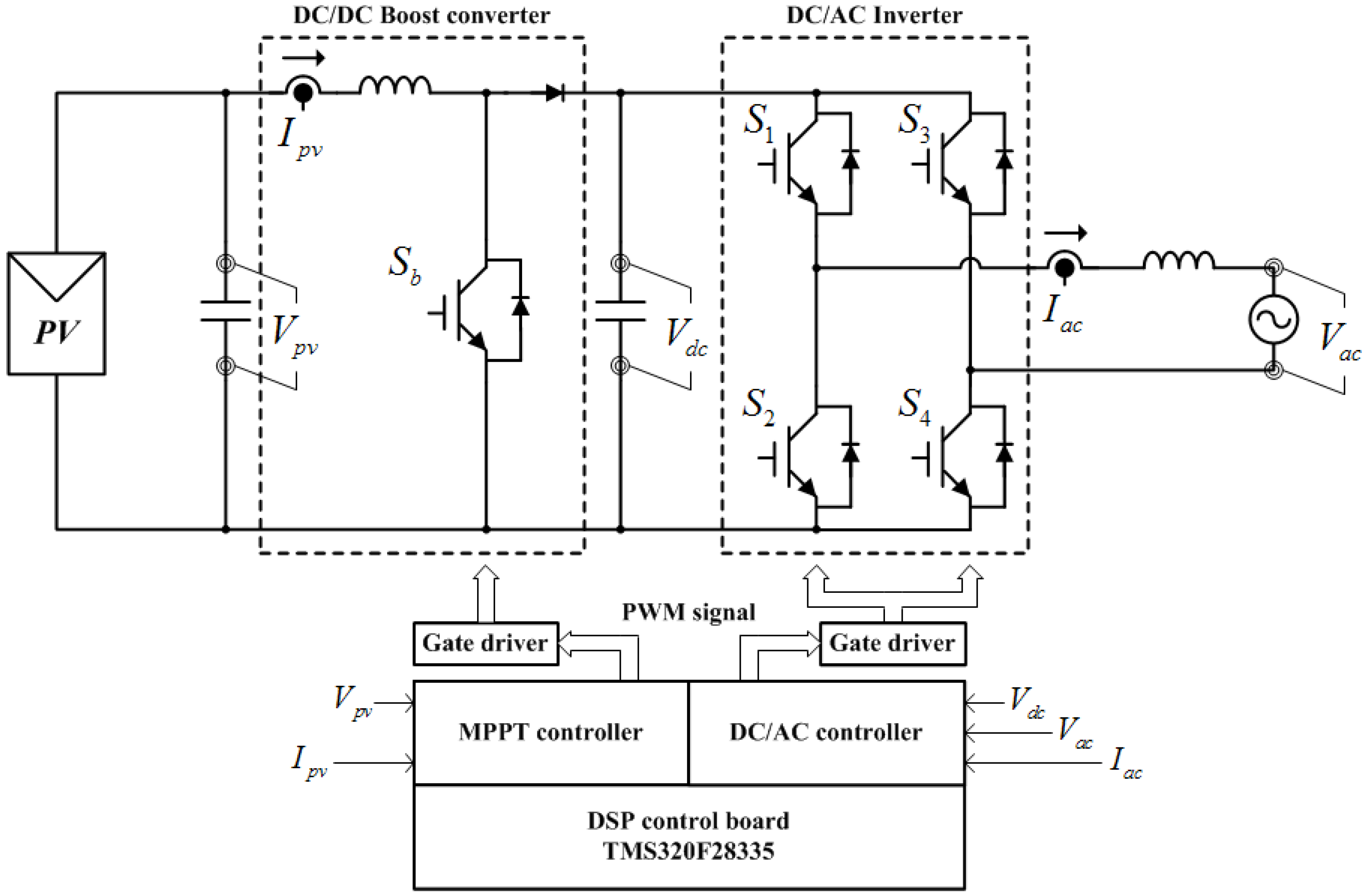
Figure 1 shows a two-stage single-phase PV PCS that is commonly used. The PV PCS is composed of a PV array, DC/DC boost converter, DC-link, inverter, and inductor filter. To extract the maximum power from the PV array, the DC/DC boost converter has to perform MPPT control. In the DC/AC inverter, current control and DC-link voltage control are performed to deliver the generated power.
Figure 1.
Diagram of a two-stage single-phase PV PCS.
Figure 1.
Diagram of a two-stage single-phase PV PCS.
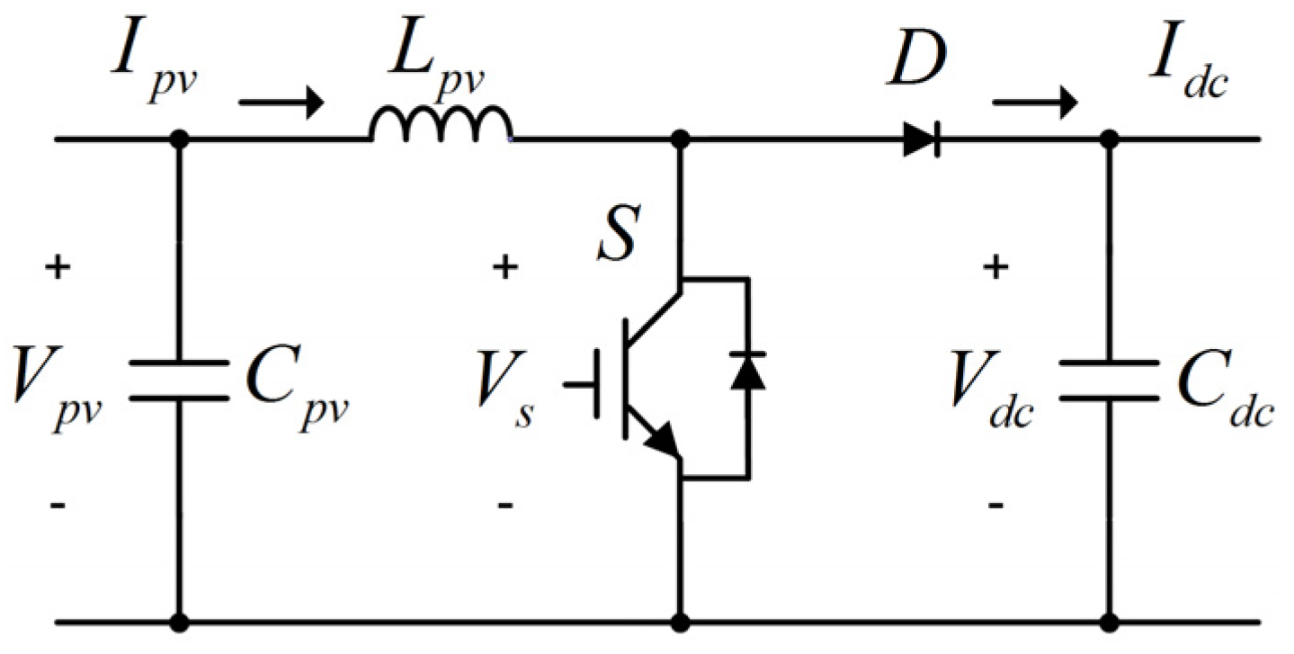
2.1. DC/DC Boost Converter
The boost converter circuit (
Figure 2) consists of a switch, diode, inductor, and capacitor. The switch
S is controlled by a gating signal of a current controller.
Figure 2.
DC/DC boost converter.
Figure 2.
DC/DC boost converter.
When the switch S is turned on, the voltage across the switch, vs, is zero during on-time DT. Therefore, the inductor voltage vL is approximately equal to the input voltage vpv and the diode voltage vD is equal to the output voltage vdc.
When
S is turned off, the voltage across the switch,
vs, is equal to the output voltage
vo and the diode voltage
vD is zero during off-time (1 −
D)
T. Hence, the inductor voltage
vL is equal to
vpv −
vdc. The inductor average voltage is given as:
where
D is the duty ratio of the switch
S.
Because the inductor average voltage is zero in a steady state, the voltage transfer ratio
Gv is:
Because the duty ratio D is between 0 and 1, the output voltage must always be higher than the input voltage.
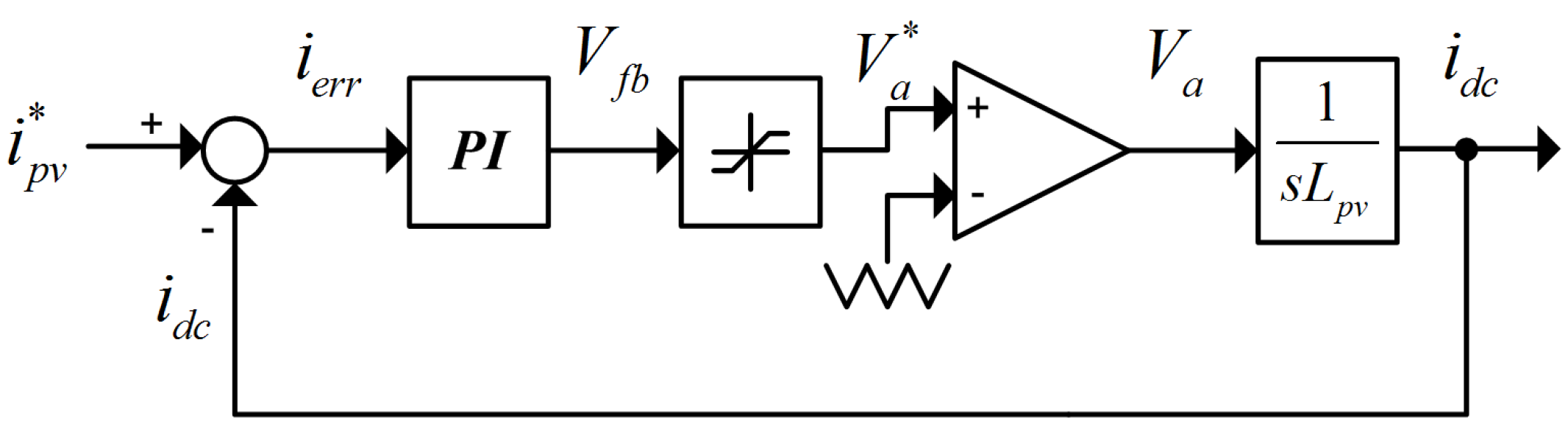
Figure 3 shows a conventional PI current controller scheme for a DC/DC boost converter. The current controller compares the inductor current
idc and a reference current
i*pv from the MPPT function. As depicted in
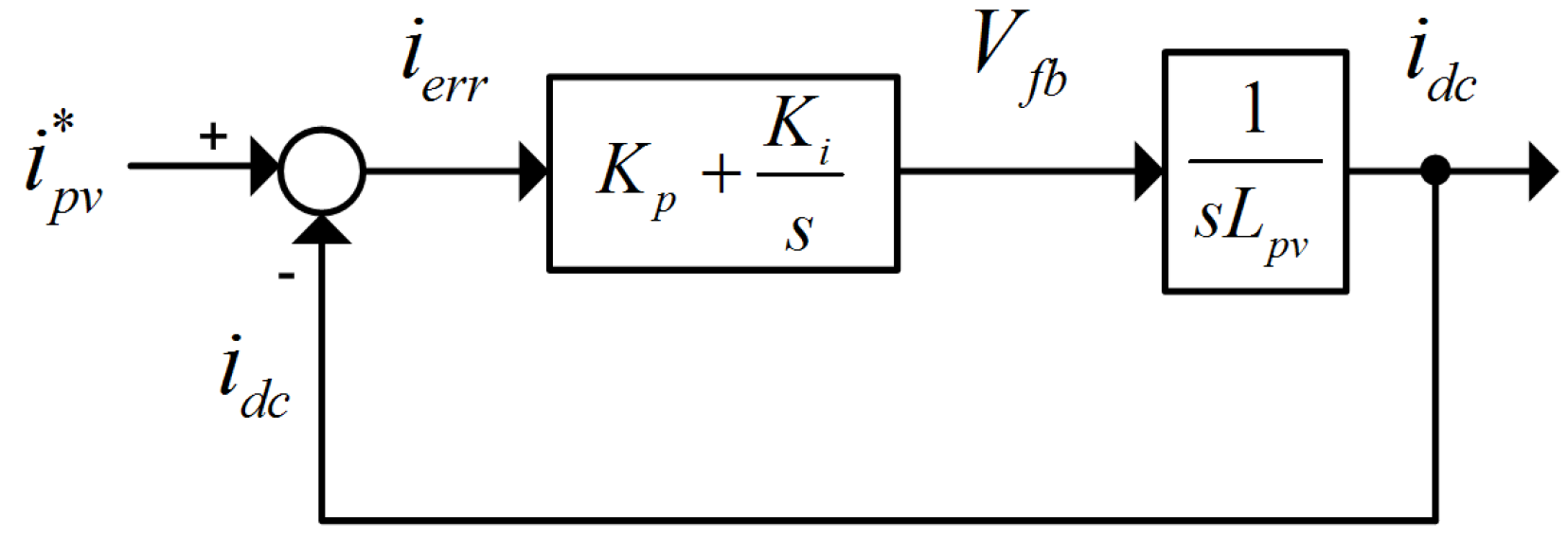
Figure 4, the transfer function is derived as:
where
Kp and
Ki are gain constants.
Figure 3.
Conventional PI current controller.
Figure 3.
Conventional PI current controller.
Figure 4.
Simplified PI current controller.
Figure 4.
Simplified PI current controller.
2.2. DC/AC Inverter
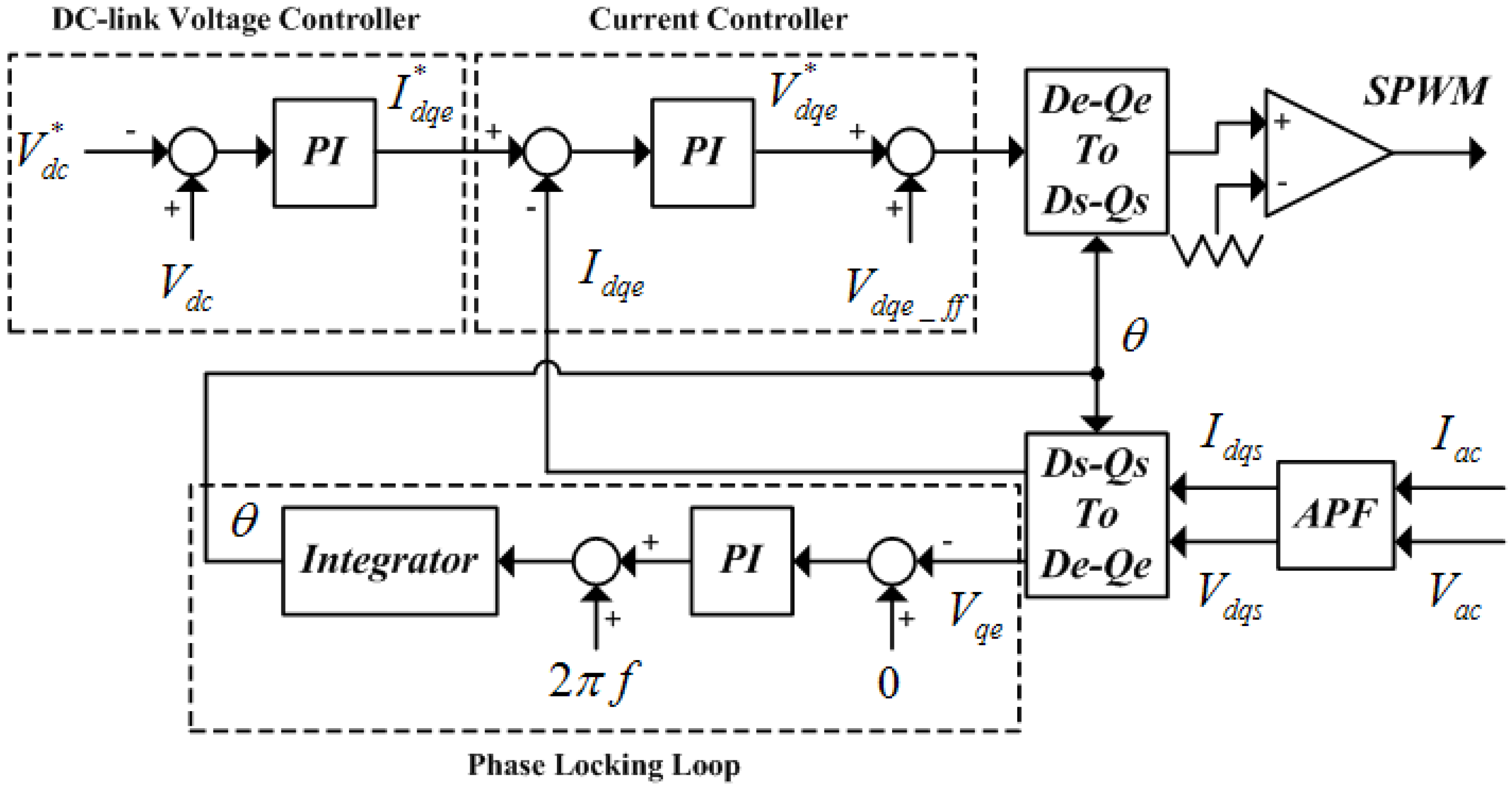
Figure 5 shows a block diagram of DC/AC inverter control for single-phase system. In the phase-locking loop (PLL) for the grid synchronization, the estimated grid angle is used for the D-Q transformation. A grid voltage and current are converted to active and reactive component using the D-Q transformation and the APF. The DC/AC inverter converts DC power into AC power. As seen from
Figure 5, the DC-link voltage controller and current controller is performed for unity power factor. As the DC-link voltage is higher than the reference DC-link voltage, the DC-link voltage controller increases the reference grid current and the output power is increased. In the contrary case, the DC-link voltage controller decreases the reference grid current and the output power is decreased.
Figure 5.
Block diagram of DC/AC inverter control for single-phase system.
Figure 5.
Block diagram of DC/AC inverter control for single-phase system.
2.3. Analysis of Second-Order Harmonic
Figure 1 shows the two-stage single-phase PV PCS. The power equations for the PV-side and grid-side are:
where
ω (= 2
πf) is the grid frequency.
If the input power and output power are equal, the input current (
Ipv) of a DC/DC boost converter can be calculated as [
8]:
Equation (6) shows that
Ipv is pulsating with the output power. The input current has a second-order harmonic at twice the fundamental frequency. Similarly,
Idc is pulsating with the output power in the DC-link. This means that the output current (
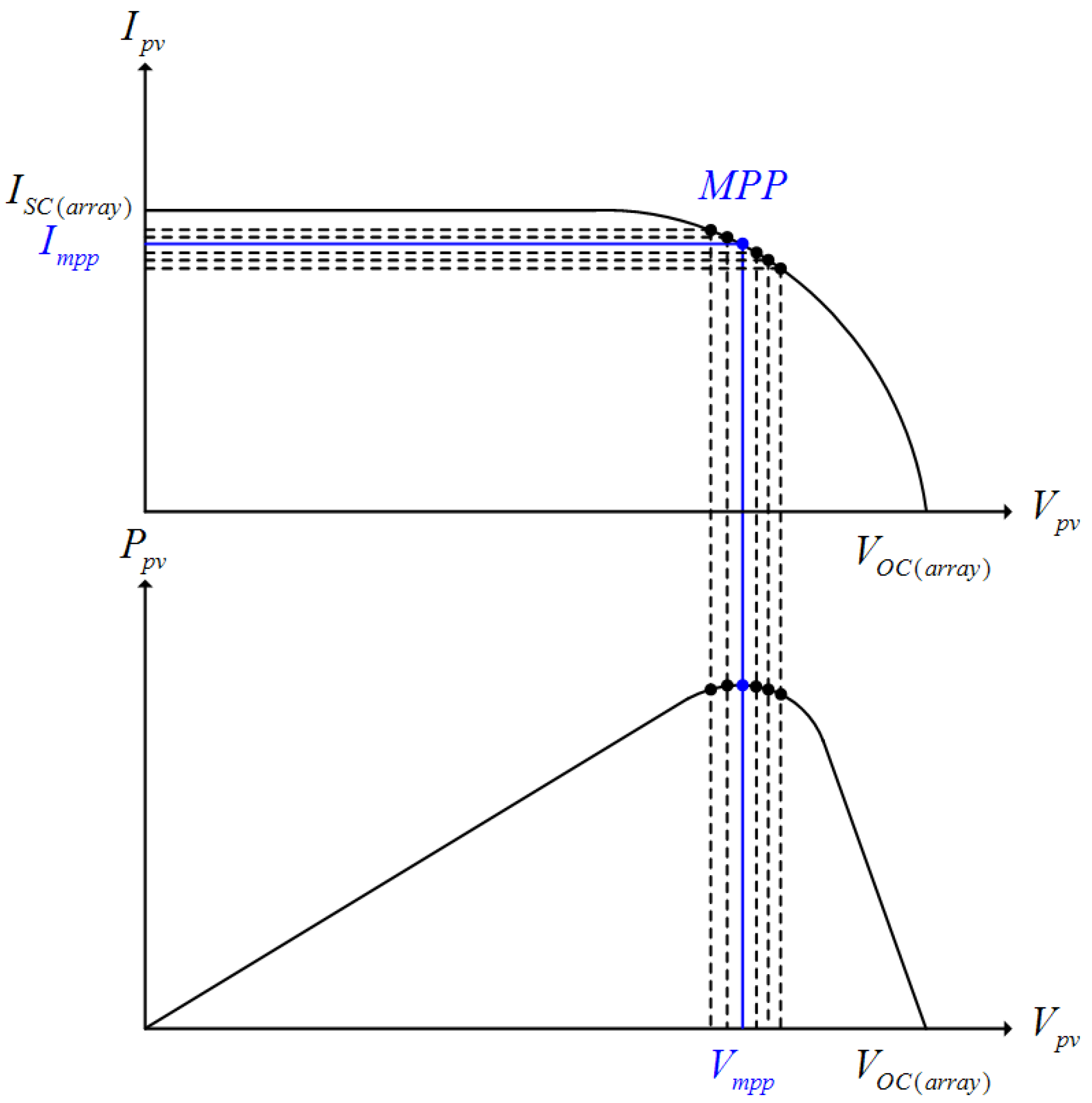
Idc) of the DC/DC boost converter also has a ripple component. If the input current has no ripple components, the operating points are fixed as shown in
Figure 6 (solid line).
However, if the input current has the ripple component, the operating points are continuously moving around a maximum power point (MPP). Therefore, the MPPT efficiency is reduced by ripples and noise [
12].
Figure 6.
Operating point of the PV array.
Figure 6.
Operating point of the PV array.
3. Proposed Second-Order Harmonic Reduction Technique
As mentioned above, the second-order harmonic inevitably occurs in single-phase systems. In [
13], the use of a large bank of energy storage capacitors has been suggested. This method can reduce the ripple component, but it causes the entire system to be expensive and bulky. An active power filter was proposed, but this method also needs extra hardware and a complex control system [
14].
In order to remove the harmonic, a ripple component can be calculated by manipulating system parameters [
8]. The calculated second-order harmonic component is added to the output of controller for the feed-forward compensation. This method can be compensated the second-order harmonic without complex calculations. However, due to changes in parameters under various conditions, the calculated second-order harmonic component is inaccurate. Therefore, the 120 Hz ripple component cannot be removed completely.
A dual-loop control method is implemented in order to reduce the second-order ripple component [
9]. In this method, a current controller is added to the existing DC-link voltage controller. In this case, the voltage loop bandwidth has to be set very low to reduce the second-order harmonic usually from 1 to 5 Hz. Owing to the lower voltage loop bandwidth, a large overshoot and undershoot of the DC-link voltage can occur during the transient-state.
3.1. PR Controller
The PR controller is used in the stationary frame unlike the PI controller. The computation sequence of the PR controller is not complex because there is no transformation from the stationary frame to synchronous frame. For these reasons, a low-cost processor can be used. In addition, when grid unbalance or a sensing error occurs, the PR controller is more robust than the PI controller. Especially, the PR controller is suitable for constant frequency operation in the grid-connected system.
Generally, the PI controller has drawbacks such as difficulty in removing the steady-state error in a stationary reference frame. The PR controller structure recently gained considerable popularity owing to its capability of eliminating steady-state error when regulating sinusoidal signals [
15,
16,
17]. Moreover, the easy implementation of a harmonic compensator without any adverse effect on the controller performance makes this controller well suited for grid-tied systems [
18].
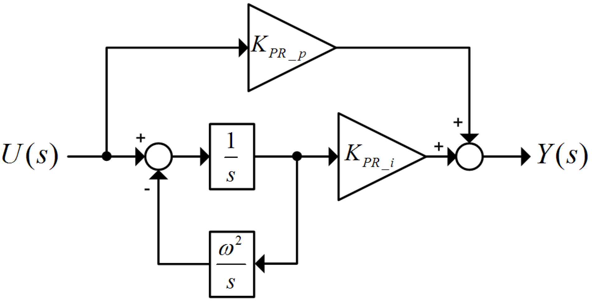
Figure 7 shows a block diagram of PR controller. The transfer function of the PR controller is defined below:
where
KPR_p and
KPR_i are gain constants and
ω (= 2
πf) is the grid frequency.
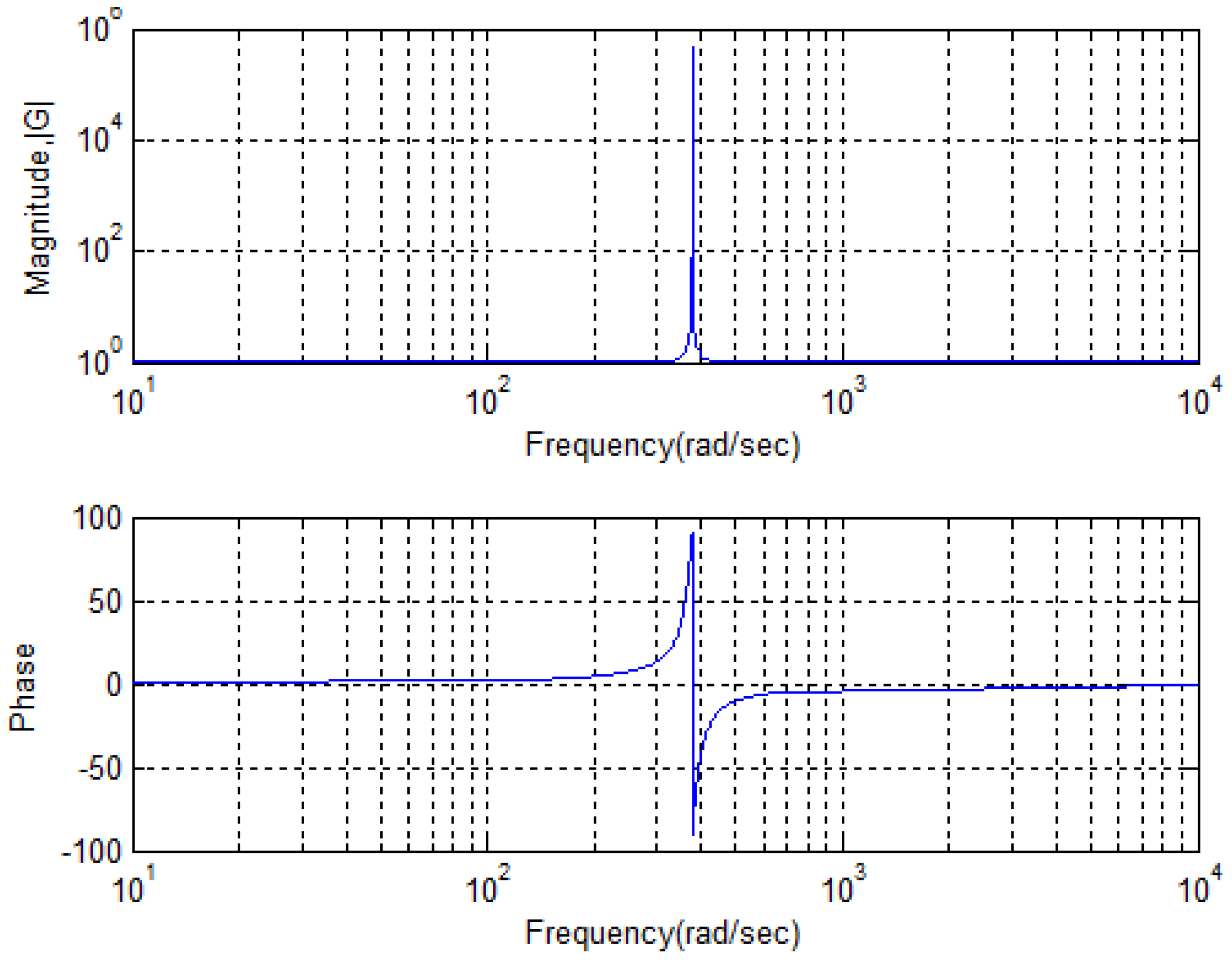
In
Figure 8, the PR controller shows a very high gain and a zero phase shift at the frequency
ω. To avoid a stability problem associated with infinite gain, an approximating (non-ideal) PR controller using a high-gain low-pass filter is used [
19]. The non-ideal PR controller can be expressed as:
where
ωc is the cut-off frequency.
Figure 8.
Bode-plot of ideal PR controller; Kp = 1, Ki = 20, ω = 377 rad/s, and ωc = 10 rad/s.
Figure 8.
Bode-plot of ideal PR controller; Kp = 1, Ki = 20, ω = 377 rad/s, and ωc = 10 rad/s.
Assuming
ωc <<
ω, equation (8) can be written as:
The non-ideal PR controller gains are set by a reasonably high finite gain for eliminating the steady-state error. Substituting
(bilinear transformation) into (9) gives the discrete transfer function of the PR controller as:
where
Ts is the sampling time and:
The digital equation of the PR controller is:
3.2. Feed-forward Compensation
Since the PR controller acts on a very narrow band around its resonant frequency
ω, a harmonic compensator for low-order harmonics can be implemented without any adverse effect on the behavior of the current controller [
1]. The harmonic reduction can also be included in the structure by cascading several generalized integrators tuned to resonate at the desired frequency
ω. The transfer function of the harmonic compensator is given by:
where
h denotes the harmonic order.
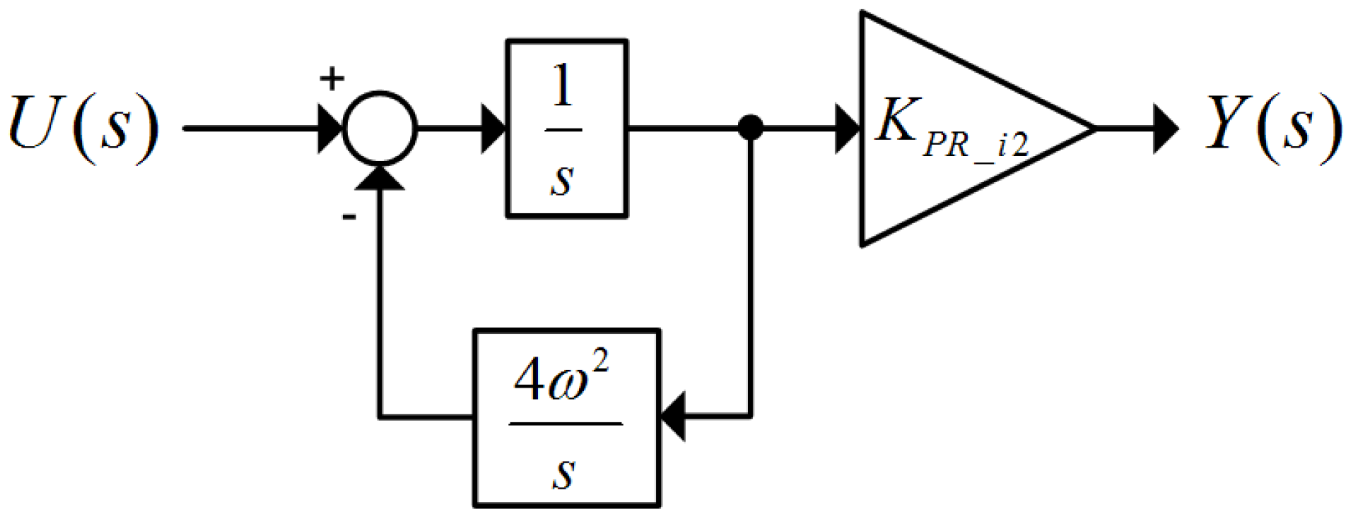
For the extraction of the second-order harmonic, the harmonic compensator should be designed as follows:
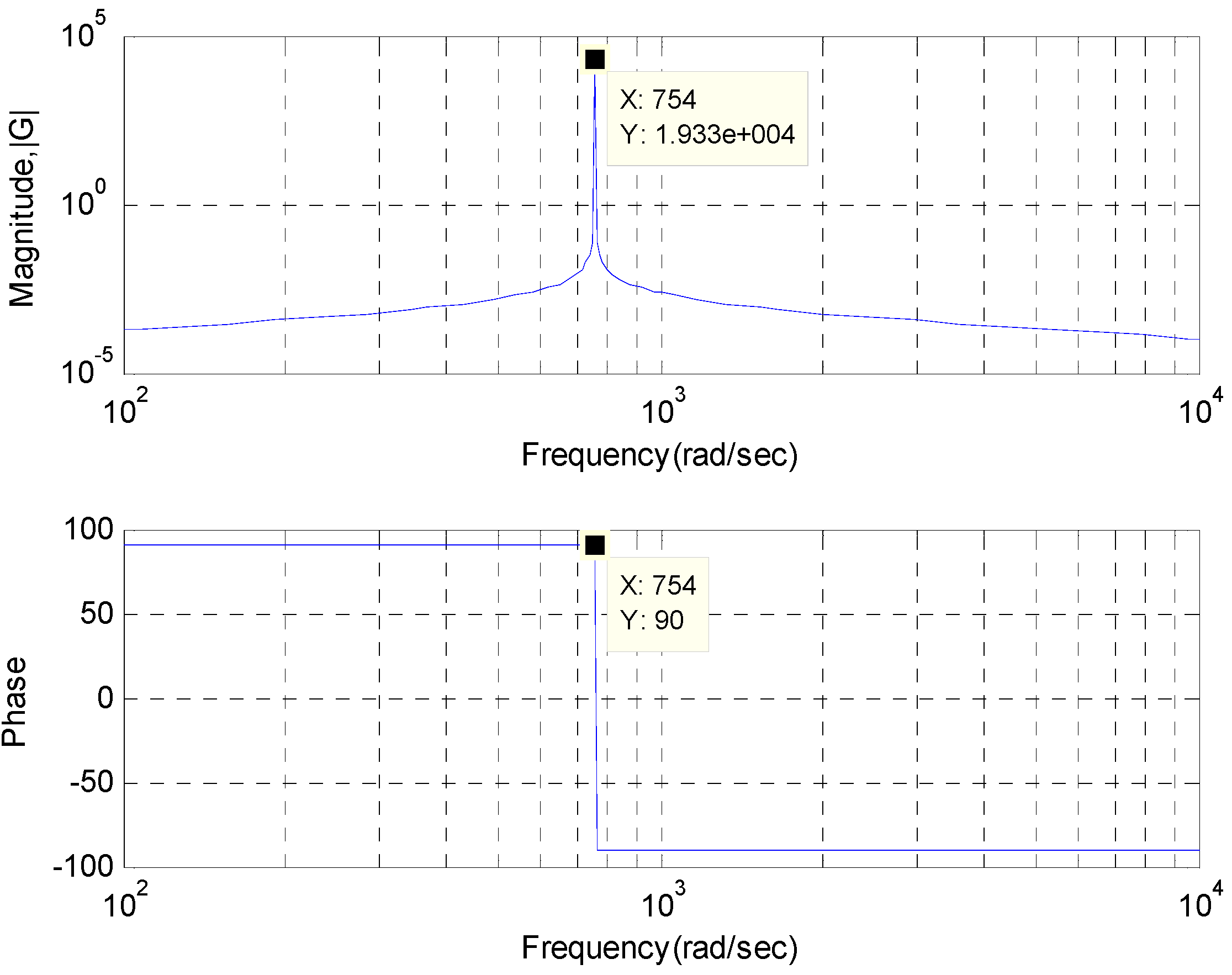
The Bode plot of the PR controller for
ω set to 120 Hz is shown in
Figure 9. It can be seen that, this controller can achieve a very high gain and a zero phase shift in a narrow frequency band (
ω = 2
πf = 2
π × 120 rad/s = 754 rad/s). The width of the frequency band depends on the integral gain constant
KPR_i2. Thus, it can also be used as a digital filter in order to compensate for the harmonics.
Figure 10 shows a block diagram of PR controller for harmonic compensation.
Figure 9.
Bode-plot of PR controller tuned for 120 Hz; Kp = 1, Ki = 20, ω = 754 rad/s, and ωc = 10 rad/s.
Figure 9.
Bode-plot of PR controller tuned for 120 Hz; Kp = 1, Ki = 20, ω = 754 rad/s, and ωc = 10 rad/s.
Figure 10.
PR controller for harmonic compensation.
Figure 10.
PR controller for harmonic compensation.
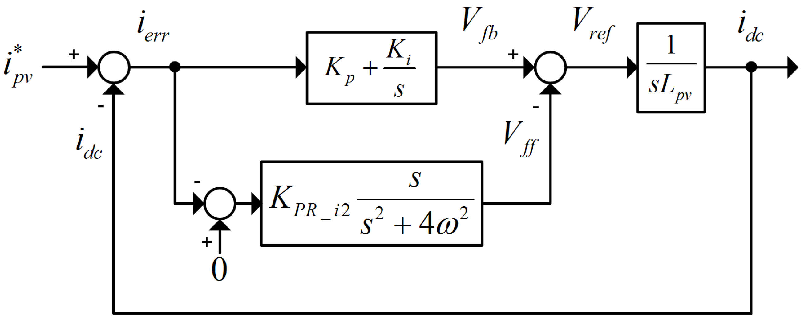
The second-order harmonic extracted from the PR controller can be used to compensate for the 120 Hz ripple. As shown in
Figure 11, the extracted second-order harmonic is added to the output of the PI controller as a feed-forward component.
Figure 11.
PI current controller with feed-forward compensation.
Figure 11.
PI current controller with feed-forward compensation.
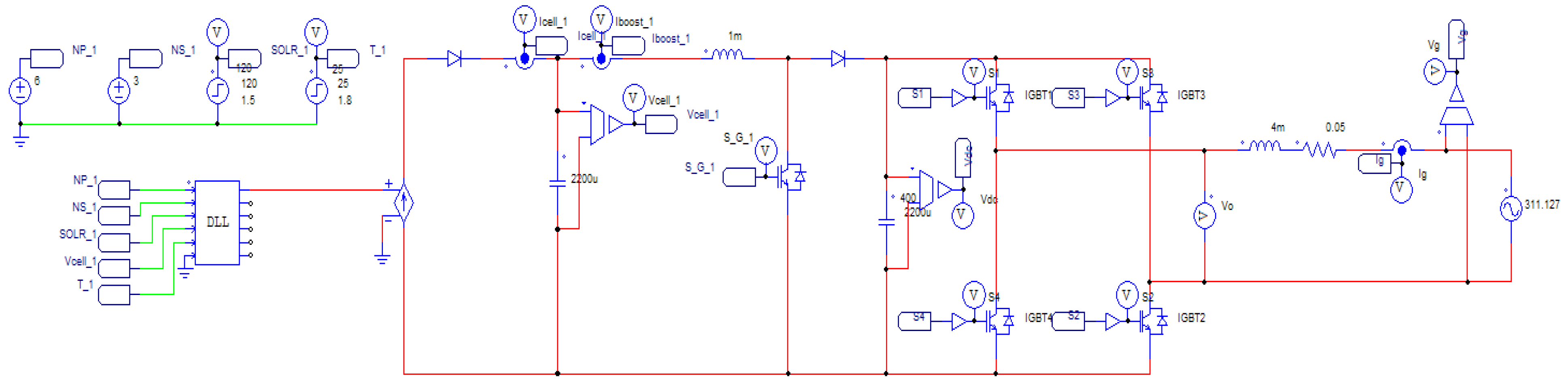
4. Simulation Results
The proposed algorithm was verified by performing a simulation using PSIM software as shown in
Figure 12. The parameters used in the simulation are listed in
Table 1.
Figure 12.
Simulation diagram.
Figure 12.
Simulation diagram.
Table 1.
Parameters of the simulation.
Table 1.
Parameters of the simulation.
| | Parameter | Value |
|---|
| Grid phase voltage | Emax | 311.127 [V] |
| Grid frequency | f | 60 [Hz] |
| Sampling period | Ts | 100 [µs] |
| Grid-side inductor | Lg | 4 [mH] |
| Grid-side resistor | Rg | 0.05 [Ω] |
| Grid-side switch frequency | fsw_g | 5 [kHz] |
| DC-link capacitor | Cdc | 2,200 [µF] |
| PV-side inductor | Lpv | 1 [mH] |
| PV-side capacitor | Cpv | 2,200 [µF] |
| PV-side switch frequency | fsw_pv | 5 [kHz] |
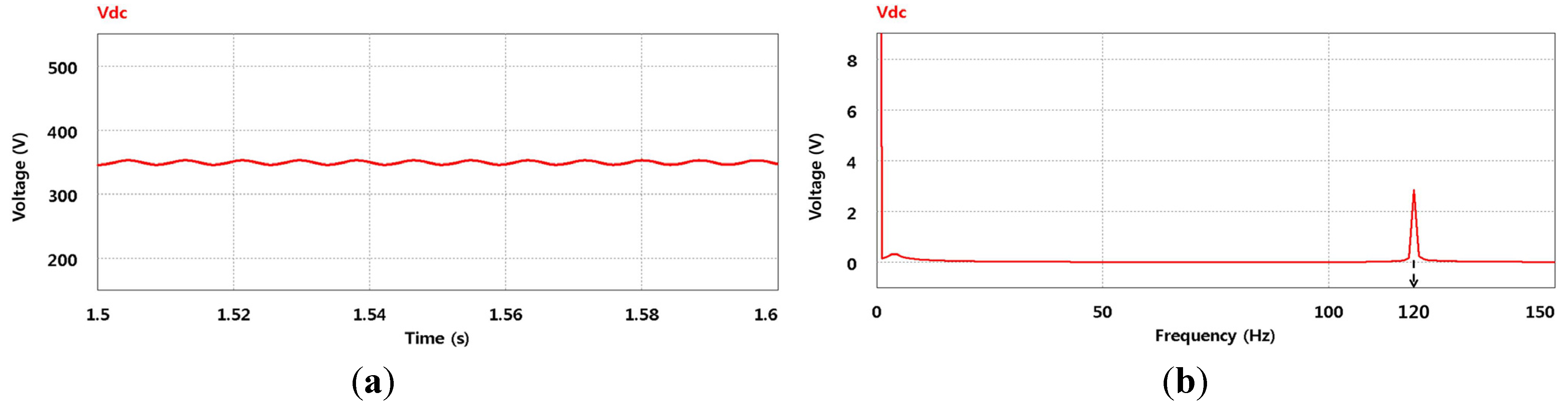
Figure 13 shows the simulation waveform of the DC-link voltage. Under the influence of the second-order harmonic, the DC-link voltage is pulsating, as shown in
Figure 13(a). It is found that the ripple component in the frequency domain represents the second-order harmonic as shown in
Figure 13(b).
Figure 13.
Simulation waveform of DC-link voltage. (a) Time domain; (b) frequency domain.
Figure 13.
Simulation waveform of DC-link voltage. (a) Time domain; (b) frequency domain.
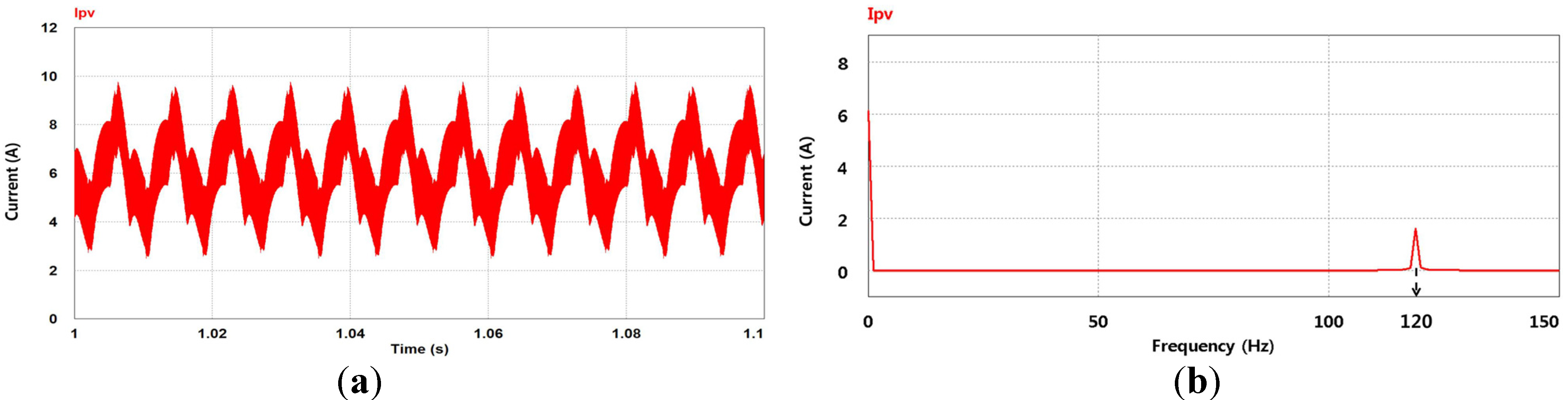
Figure 14 shows the simulation waveform of the PV current without compensation. The PV current is pulsating with the DC-link voltage, as shown in
Figure 14(a). The second-order harmonic can be seen in the frequency domain, as shown in
Figure 14(b).
Figure 14.
Simulation waveform of PV current without compensation. (a) Time domain; (b) frequency domain.
Figure 14.
Simulation waveform of PV current without compensation. (a) Time domain; (b) frequency domain.
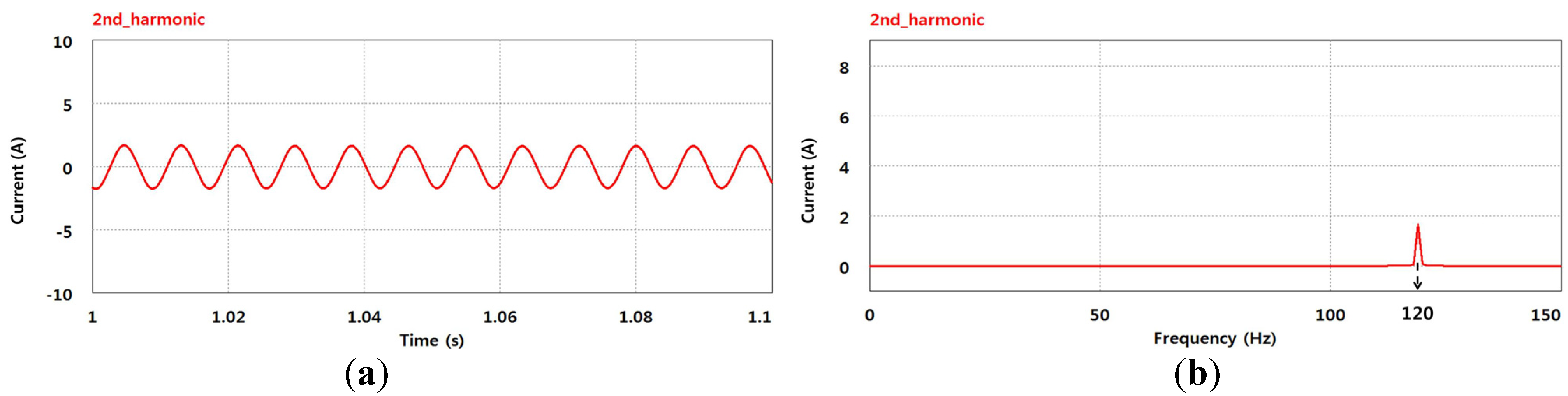
The extracted second-order harmonic component using the PR controller is shown in
Figure 15. As seen from this figure, the harmonic component can be extracted accurately. The extracted component is used to mitigate the second-order harmonic in the PV current.
Figure 15.
Simulation waveform of the second-order harmonic component. (a) Time domain; (b) frequency domain.
Figure 15.
Simulation waveform of the second-order harmonic component. (a) Time domain; (b) frequency domain.
Figure 16 shows the simulation waveform of the PV current with compensation. It shows that the current ripples are reduced. Therefore, the effectiveness of the second-order harmonic reduction with the proposed feed-forward compensation is verified.
Figure 16.
Simulation waveform of PV current with compensation. (a) Time domain; (b) frequency domain.
Figure 16.
Simulation waveform of PV current with compensation. (a) Time domain; (b) frequency domain.
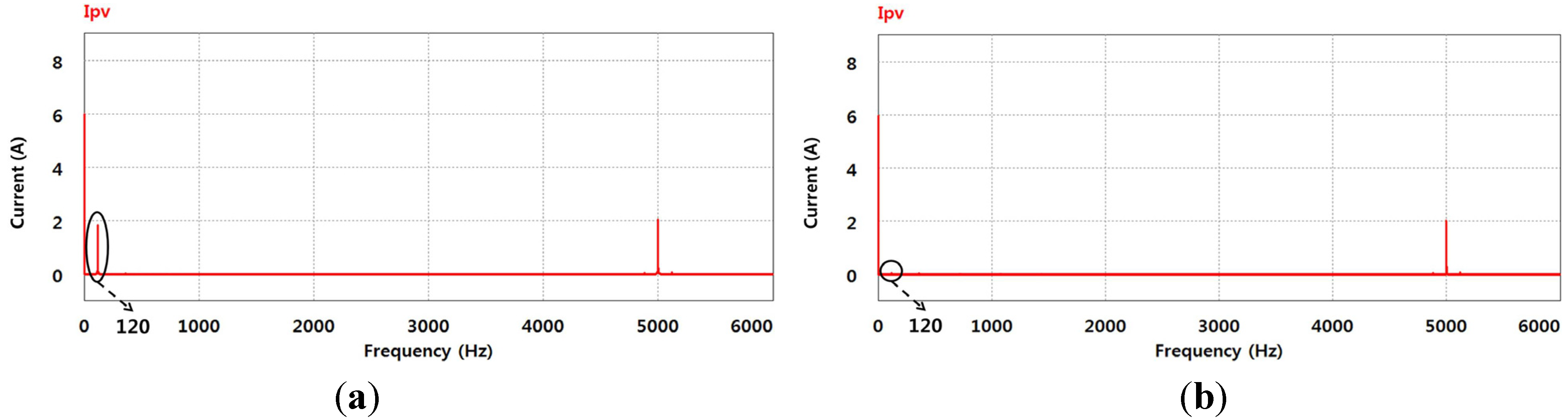
Figure 17 shows the simulation FFT waveform of the PV current before and after the harmonic compensation. In
Figure 17, the switching frequency is 5 kHz. It can be seen that only the second-order harmonic have been compensated.
Figure 17.
Simulation FFT waveform of PV current. (a) Without compensation; (b) with compensation.
Figure 17.
Simulation FFT waveform of PV current. (a) Without compensation; (b) with compensation.
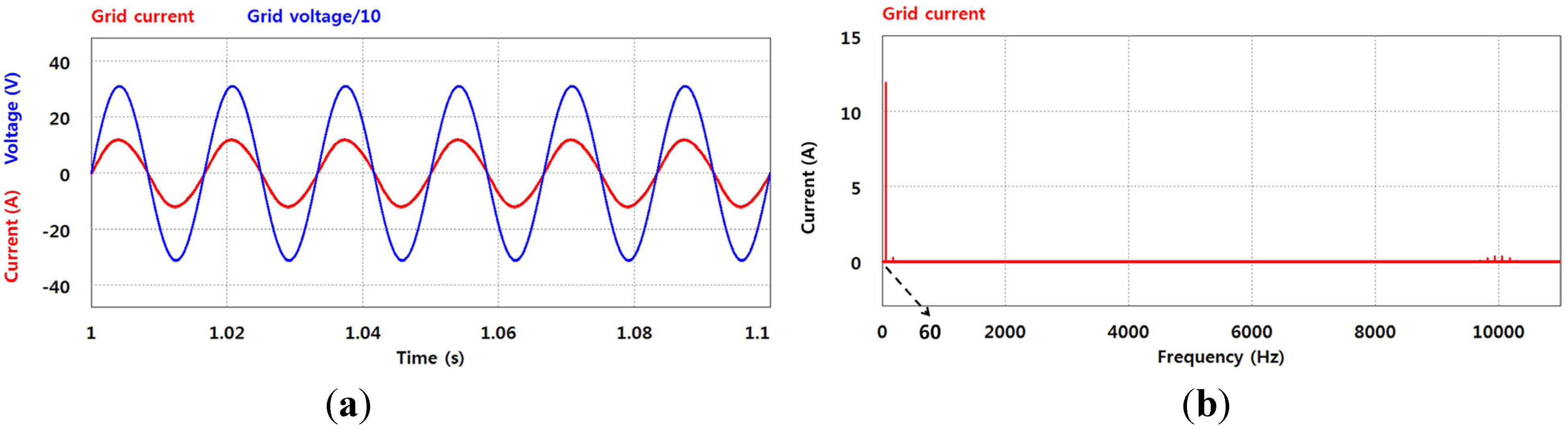
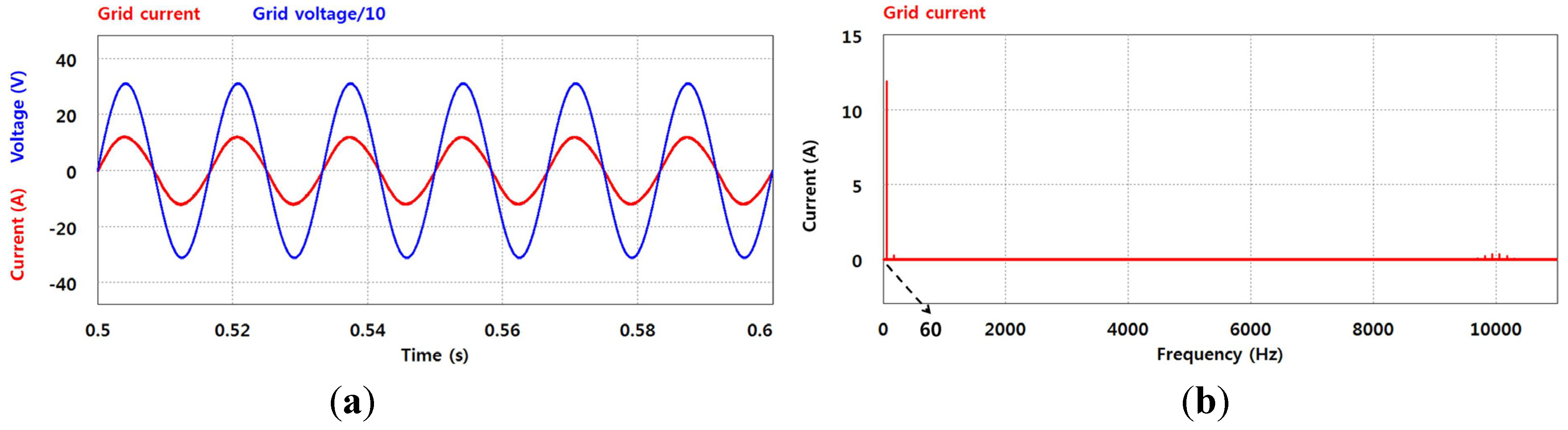
Figure 18 and
Figure 19 show the simulation waveform of the grid current and voltage before and after the compensation. It shows that a proposed algorithm does not any bad effect on the grid current and voltage. Due to the large capacitance of the DC-link capacitor, the proposed algorithm does not affect the grid-side. As seen from these figures, the current controller is performed for unity power factor.
Figure 18.
Simulation waveform of the grid current and voltage without compensation. (a) Time domain; (b) frequency domain.
Figure 18.
Simulation waveform of the grid current and voltage without compensation. (a) Time domain; (b) frequency domain.
Figure 19.
Simulation waveform of the grid current and voltage with compensation. (a) Time domain; (b) frequency domain.
Figure 19.
Simulation waveform of the grid current and voltage with compensation. (a) Time domain; (b) frequency domain.
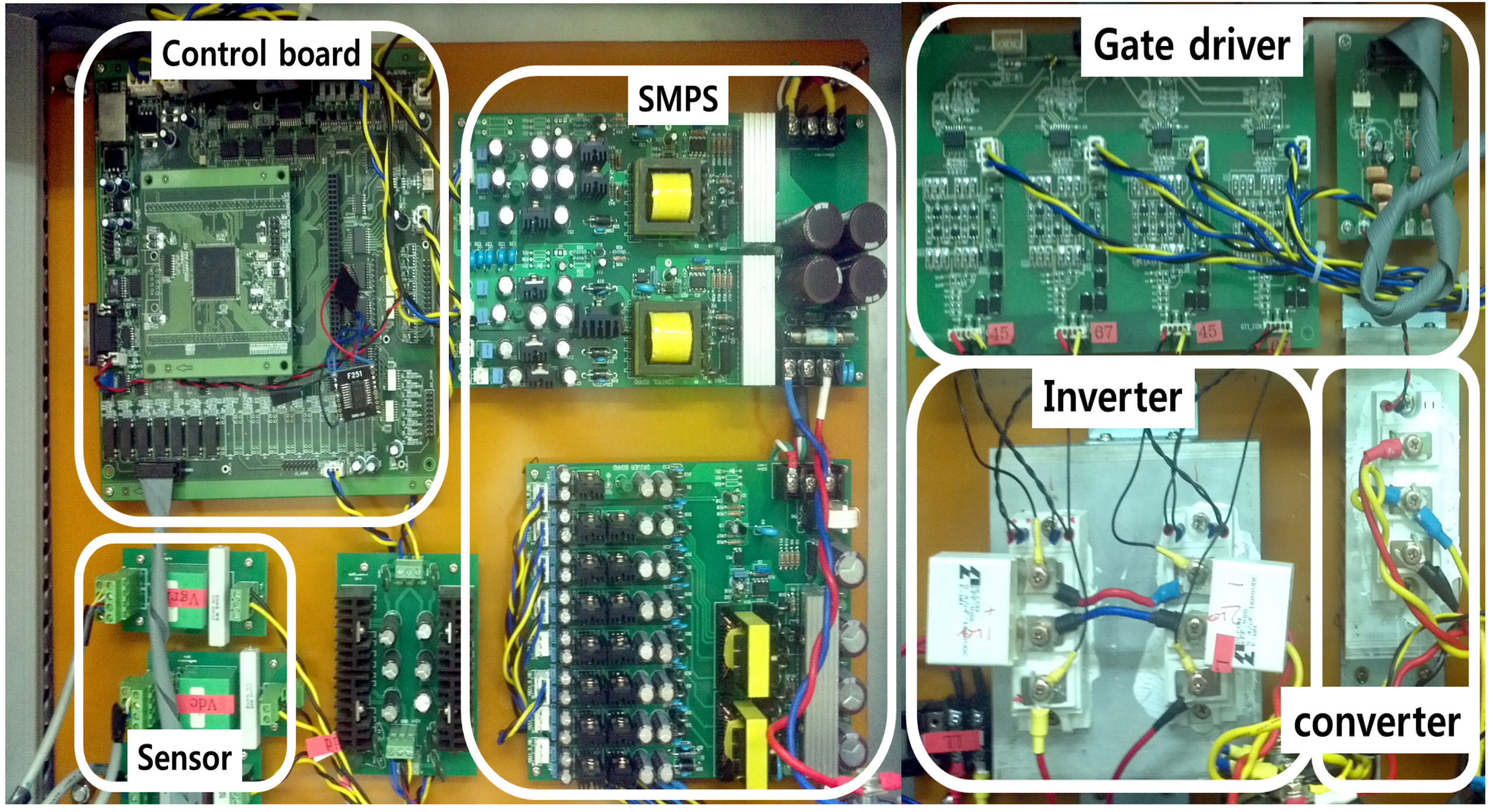
5. Experimental Results
The experiments were implemented on a PV PCS as shown in
Figure 20. The proposed method was programmed on a TMS320F28335 digital signal processor (DSP). The experimental parameters were the same as the simulation values.
Figure 20.
Experimental set.
Figure 20.
Experimental set.
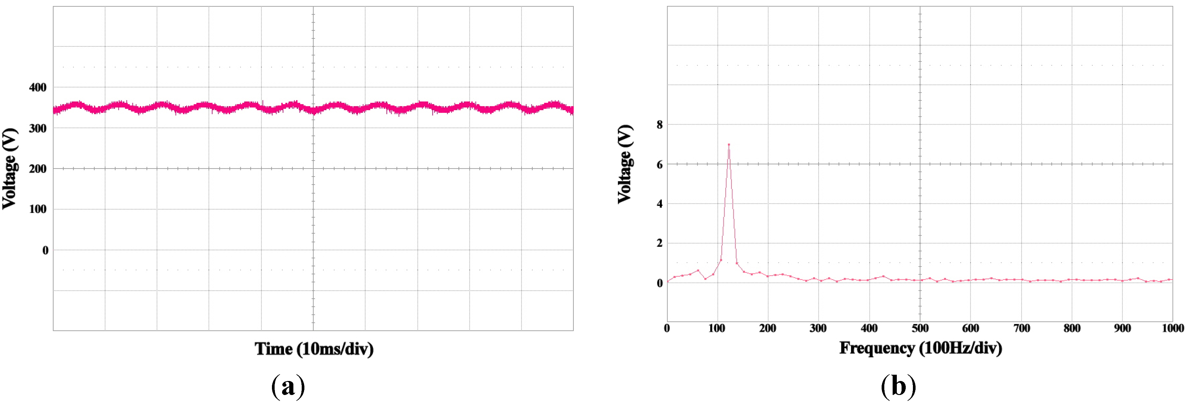
Figure 21 shows the experimental waveform with the DC-link voltage.
Figure 21(a) shows the ripple of the DC-link voltage.
Figure 21(b) shows the magnitude of the 120 Hz component of the DC-link voltage. It is seen that a ripple component with a magnitude of approximately 7 V is included.
Figure 21.
Magnitude of DC-link voltage. (a) Time domain; (b) frequency domain.
Figure 21.
Magnitude of DC-link voltage. (a) Time domain; (b) frequency domain.
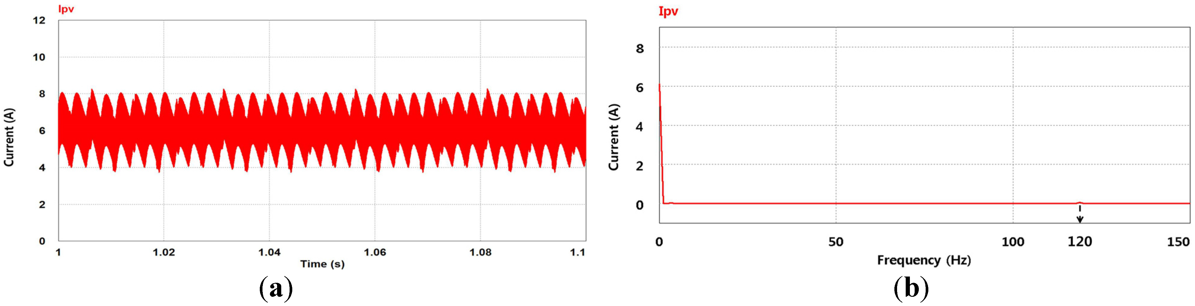
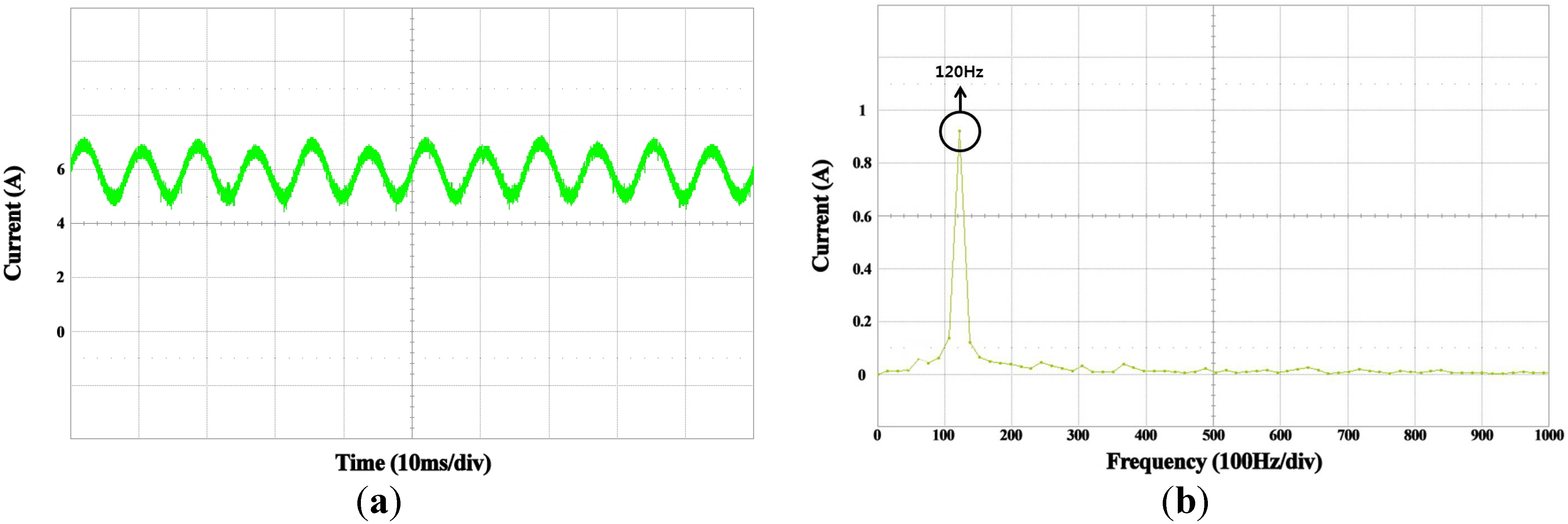
Because of the ripple component, the PV current is pulsating as shown in
Figure 22. The PV current is 6 A with ±0.95 A (15.8%) current variation. To compensate for the ripple component, the PR controller extracts the second-order harmonic component from the PV current.
Figure 23 shows the extracted component is exactly 120 Hz.
Figure 22.
Magnitude of PV current without compensation. (a) Time domain; (b) frequency domain.
Figure 22.
Magnitude of PV current without compensation. (a) Time domain; (b) frequency domain.
Figure 23.
Magnitude of the second-order harmonic component. (a) Time domain; (b) frequency domain.
Figure 23.
Magnitude of the second-order harmonic component. (a) Time domain; (b) frequency domain.
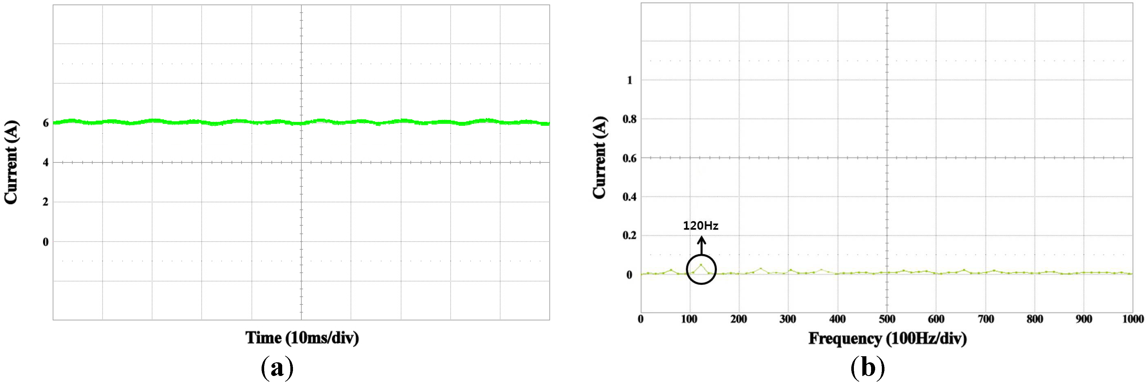
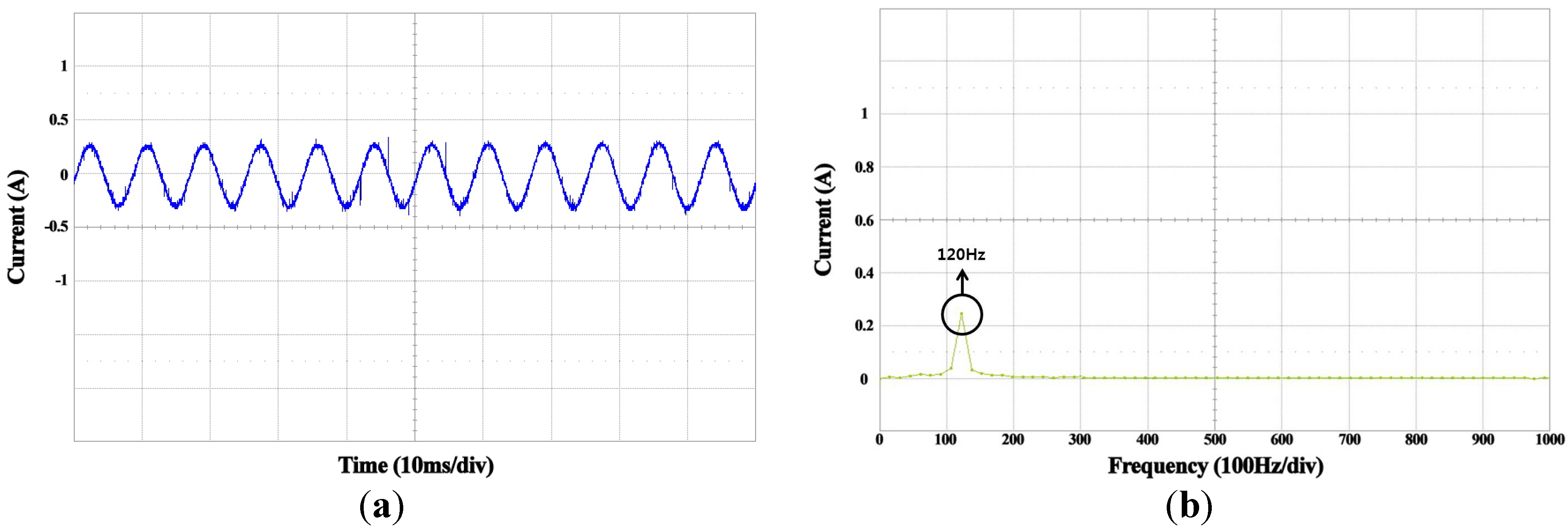
Figure 24 shows the result of the proposed feed-forward compensation using the PR controller. In
Figure 24(a), the PV current seems to be composed of only the DC component. The PV current is 6 A with ±0.05 A (0.008%) current variation.
Figure 24(b) shows that the second-order harmonic is almost removed in the frequency domain.
Figure 24.
Magnitude of PV current with compensation. (a) Time domain; (b) frequency domain.
Figure 24.
Magnitude of PV current with compensation. (a) Time domain; (b) frequency domain.
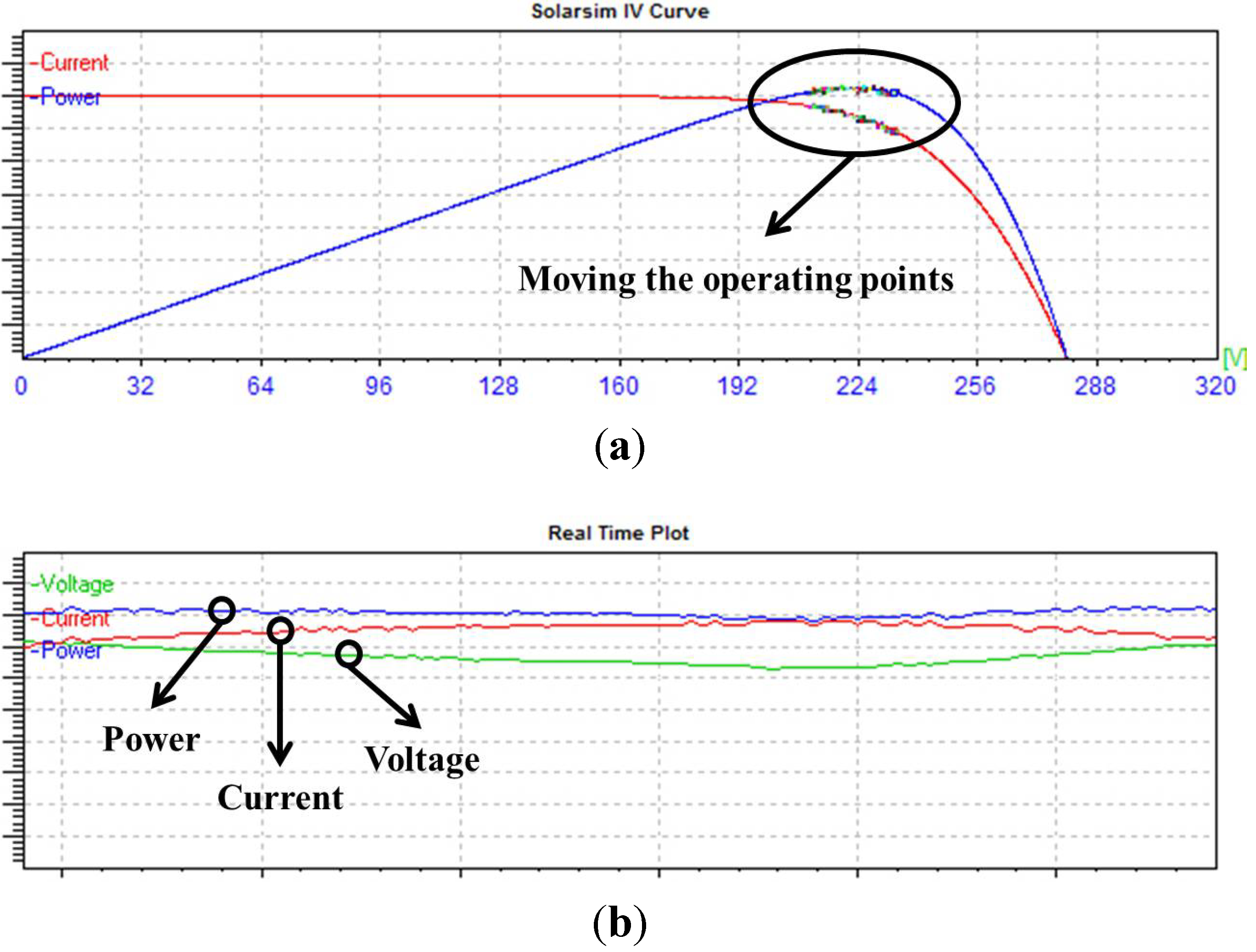
In order to verify the proposed algorithm, MPPT control is performed using the PV simulator.
Figure 25(a) shows the operating points of the PV array before the compensation. The power, current, and voltage of the PV array are observed to be changing continuously owing to the ripple component, as shown in
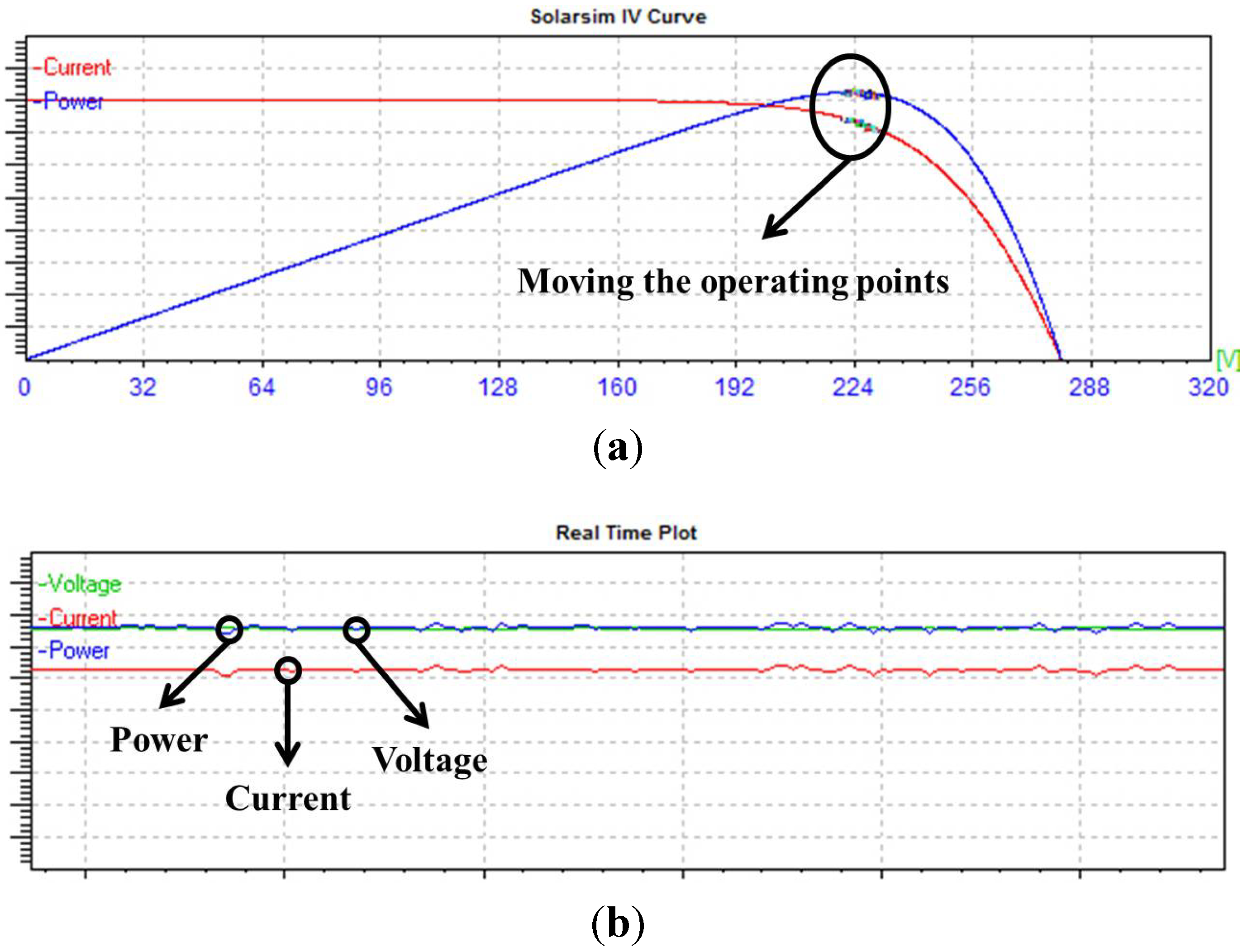
Figure 25(b). After the proposed algorithm is applied, the operating points are fixed around the MPP, as shown in
Figure 26(a). As can be seen in
Figure 26(b), the power, current, and voltage are almost constant even after compensation.
Figure 25.
Operating points of PV array before compensation. (a) P-V and I-V curve; (b) real-time plot.
Figure 25.
Operating points of PV array before compensation. (a) P-V and I-V curve; (b) real-time plot.
Figure 26.
Operating points of PV array after compensation. (a) P-V and I-V curve; (b) real-time plot.
Figure 26.
Operating points of PV array after compensation. (a) P-V and I-V curve; (b) real-time plot.
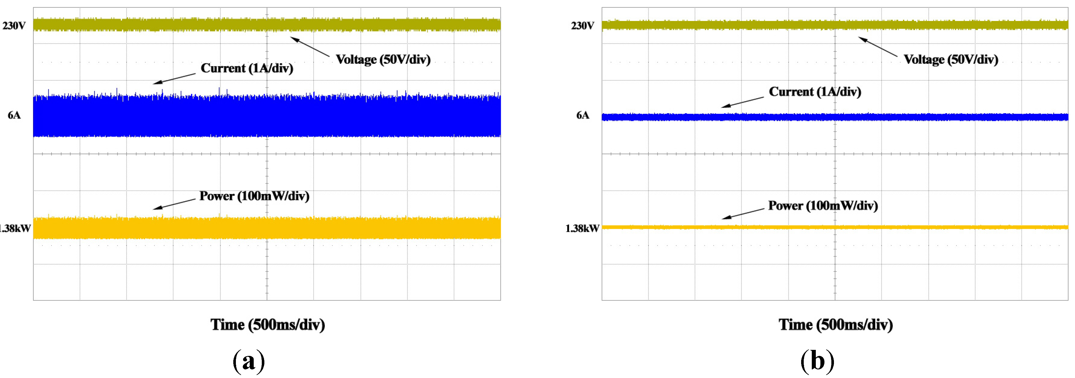
Figure 27 shows the PV voltage, current, and power during the MPPT control. As seen from
Figure 27(a), the second-order harmonic component in the PV current is pulsating with the PV power as the ripple component. In
Figure 27(a), the ripple of PV power is 70 W. The MPPT efficiency is:
In
Figure 27(b), the ripple of PV power is 20W after compensation. The MPPT efficiency is:
Figure 27.
Magnitude of a PV voltage, current, and power. (a) Without compensation; (b) with compensation.
Figure 27.
Magnitude of a PV voltage, current, and power. (a) Without compensation; (b) with compensation.


