Analytic Modeling of Vehicle Fuel Consumption

Abstract

An analytical method of evaluating vehicle fuel consumption under standard operating conditions is presented. In the proposed model, vehicle fuel consumption is separated into two different operating modes: cruising at constant speed and acceleration. In each of these modes fuel consumption is calculated based on the instantaneous engine efficiency, approximated using an analytical function rather than typically considered consumption map. The approximation is based on speed-power decoupling, employing two single dimension polynomials instead of a two-dimensional lookup table. The adequacy and accuracy of the model is verified using experimental calculations. Moreover, it is shown that the effect of various design parameters on vehicle fuel consumption can be studied utilizing the proposed model.

1. Introduction

Evaluating fuel efficiency is an important procedure during ground vehicle design and operation. Based on this evaluation, usually performed via mathematical modeling and simulation, the main construction parameters of the vehicle may be determined at the design stage and steps to reduce fuel consumption may be taken. Since one of vehicle design main goals is minimizing fuel consumption for expected operating conditions, development of analytical models that allow accurate prediction of vehicle consumption appears to be highly desirable.

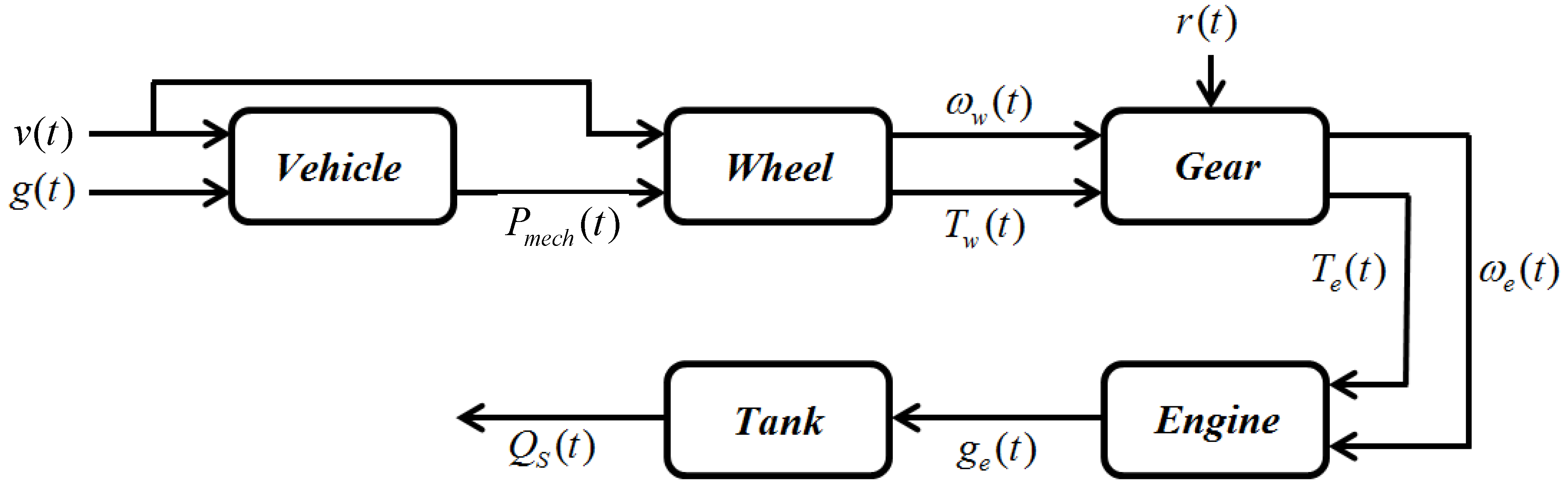
A well-known approach to estimating fuel consumption is inverse simulation [1,2,3,4], where the driving cycle-to-tank chain is represented by power transferring functional blocks with predetermined efficiency, as shown in Figure 1.

Figure 1. Inverse simulation flow. v(t)—driving speed versus time (driving profile); g(t)—road grade versus time (driving profile); P_mech(t)—mechanical power on the wheel; ω_w(t)—wheel angular speed; T_w(t)—mechanical torque on the wheel; r(t)—gear ratio; ω_e(t)—engine speed; T_e(t)—engine torque; g_e(t)—specific fuel consumption.

Figure 1. Inverse simulation flow. v(t)—driving speed versus time (driving profile); g(t)—road grade versus time (driving profile); P_mech(t)—mechanical power on the wheel; ω_w(t)—wheel angular speed; T_w(t)—mechanical torque on the wheel; r(t)—gear ratio; ω_e(t)—engine speed; T_e(t)—engine torque; g_e(t)—specific fuel consumption.

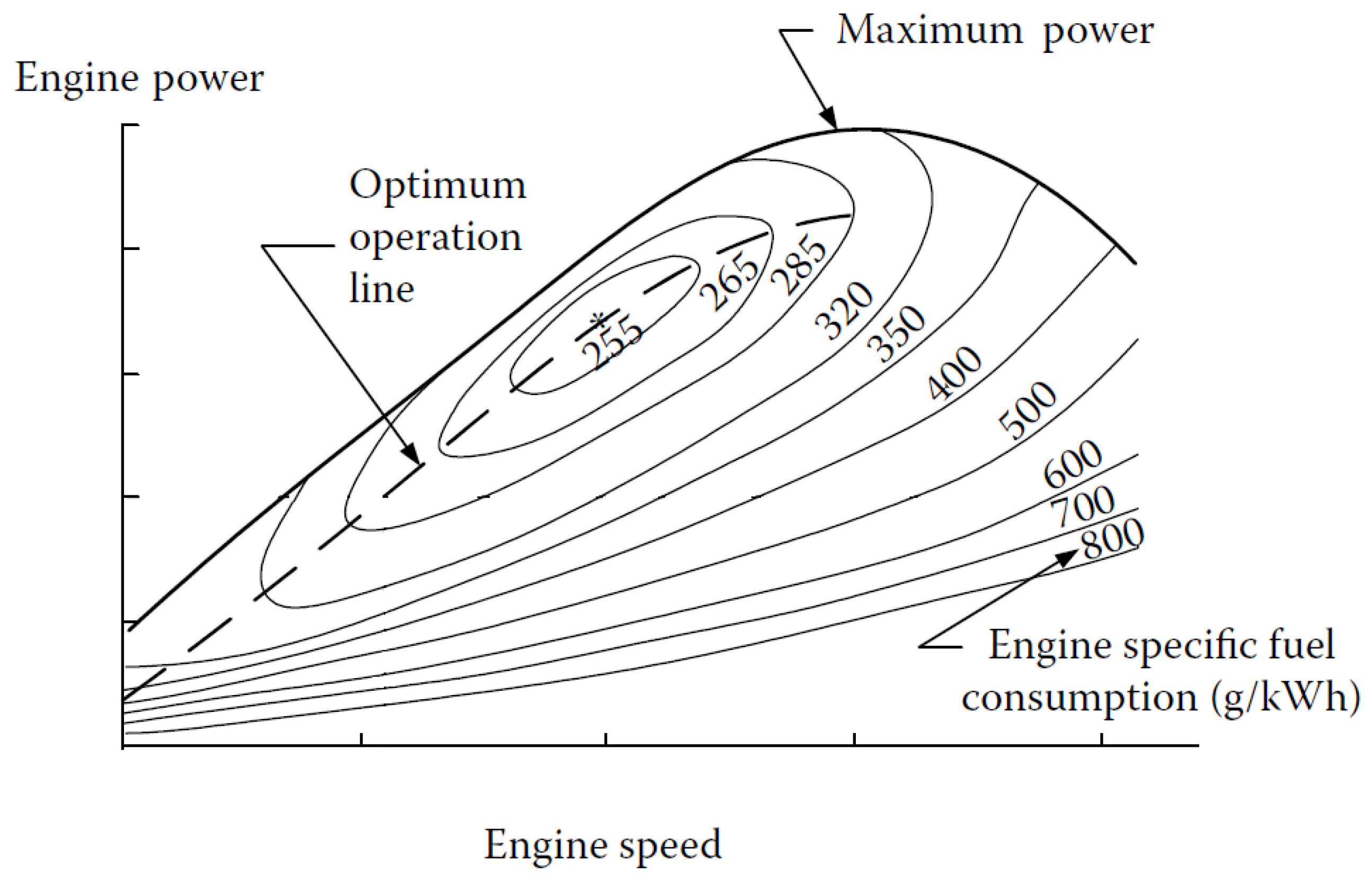
Engine specific fuel consumption is presented for illustration in Figure 2. It is usually represented by an appropriate two-dimensional lookup table, rather than obtained analytically. Alternatively, a similar two-dimensional map is often used for expressing engine efficiency rather than specific fuel consumption. Hence, simulation software must be used in order to determine the vehicle mileage. It would be more convenient if the fuel consumption could be determined from analytic expressions as much as possible, reducing the dependence on empirical simulation.

Figure 2. Typical internal combustion engine specific fuel consumption map [3].

Figure 2. Typical internal combustion engine specific fuel consumption map [3].

Attempts for creating mathematical models for estimating fuel efficiency have been widely made in the literature. For example, it was proposed in [5,6] to evaluate fuel consumption Q_S measured in liters per 100 km via the following relation:

$$Q_S=\frac{g_e\cdot (P_{rl}+P_w+P_a)}{10\cdot V_a\cdot {\eta }_T\cdot {\rho }_f},$$

(1)

where g_e is the optimal specific fuel consumption, g∙kWh⁻¹; P_rl is the power required to overcome the rolling resistance of the road, kW; P_w is the power required to overcome the resistance of the air, kW; P_a is the power required to overcome the resistance of the inertial acceleration, kW; η_T is the efficiency of the transmission; ρ_f is the fuel density, kg∙L⁻¹; V_a is the average speed of the vehicle, km∙h⁻¹.

Equation (1) assumes that the specific fuel consumption is constant and minimal. In [7,8] it is proposed to calculate fuel consumption based on specific hourly fuel consumption and energy expenditure, while the authors of [2,3] have suggested determining energy expenditure based on a computer simulation software ADVISOR; good results were obtained for the qualitative analysis of fuel economy. Energy expenditure determination based on statistical modeling was proposed in [1,2,3,4].

Particularly noteworthy is the work of Guzzella et al. [3], where mechanical energy consumption of vehicles for the European Driving Cycle MVEG-95 was determined. The authors proposed the following relation:

$$E_{MVEG-95}\approx A_f{c}_D\cdot 1.9\cdot {10}^4+m_v{f}_r\cdot 8.4\cdot {10}^2+m_v\cdot 10[\text{kJ/100\hspace{0.17em}km}]$$

(2)

where m_v is car mass, kg; f_r is the rolling resistance coefficient; c_D is the coefficient of aerodynamic resistance of the car; A_f is the characteristic area of the car, m².

The first term in the right-hand side of Equation (2) is the energy required for overcoming the resistance of the air, the second term is the energy required for overcoming the resistance of the road, and the third term is the energy required for overcoming the inertial acceleration.

Basically, the bottleneck of all the proposed approaches is the need to include an engine consumption map, which was overcome by assuming constant specific fuel consumption for all operating modes, which is obviously inaccurate. The current work is interesting from a methodological point of view, since an attempt is being made to analytically calculate energy expenditure and fuel consumption, taking into account the instantaneous specific fuel consumption, approximated by two generalized single dimension polynomial functions. In the literature, e.g., [9,10], multiple dependencies of fuel consumption are constructed based on experimental data (approximation), but their purpose is largely confined to analyzing the influence of various factors on the fuel consumption of a specific vehicle, not theoretical generalizations.

Currently, the major set of regulations governing vehicle operating modes for estimating fuel consumption of vehicles are the rules of the UN Economic Commission for Europe [11]. The above mentioned models and formulas for calculating fuel consumption, which do not take into consideration the changes in the mode of motion, are unfit for evaluating fuel consumption in accordance with the accepted regulations. Development of a mathematical model which can be used for this purpose is the main contribution of this article.

The rest of the manuscript is organized as follows. In Section 2, the proposed model for calculating fuel consumption in accordance with UN ECE regulations is described. In this model fuel consumption is determined separately for two different vehicle operating modes: constant speed and accelerations.

In Section 3, verification of the adequacy and accuracy of the obtained formula is presented. To assess it, calculation of fuel consumption using the derived formula was carried out and the results were compared to experimental data provided by the manufacturers. In order to carry out calculations via the proposed formula, parameters common for all automobiles are first identified. The vehicle-specific parameters used are the type of engine, automobile mass, maximum power and shaft speed at maximum power. Based on the comparison of calculations carried out using the proposed model to data from the manufacturers, it is concluded that the proposed mathematical model is suitable for practical use.

The 4th section illustrates the possibilities opened up by the utilization of the proposed model. An analysis of the effect of various design and operational parameters on fuel consumption is carried out based on the model.

2. Estimating Fuel Consumption

A vehicle’s energy expenditure on a flat road consists of three parts, the first one being the energy required for overcoming the resistance of the air, the second—the energy required for overcoming the resistance of the road, and the third—the energy required for overcoming the resistance of the inertial acceleration. As stated in the introduction, the automobile engine operates in two main modes, the first one of which is movement at constant speed, and the second is acceleration. The proposed equation for estimating fuel consumption takes these into account, neglecting the fuel consumption during decelerations. In addition, the transmission efficiency is assumed to remain constant.

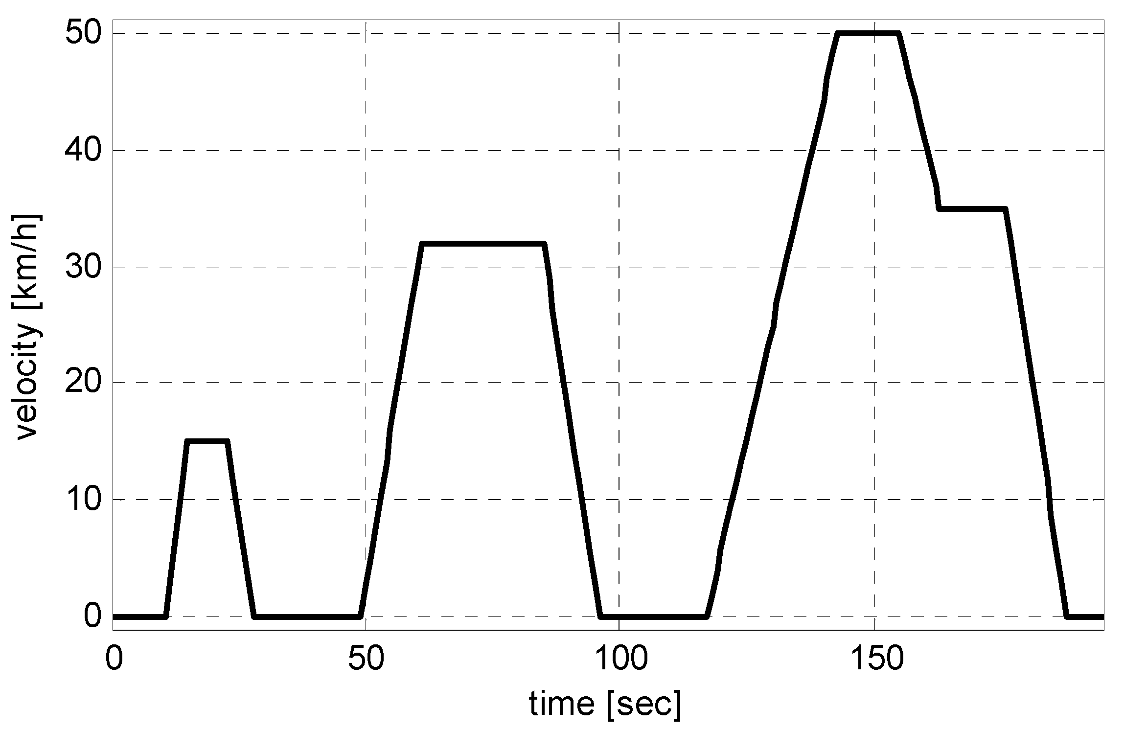
The energy expenditure on a flat road E_S is then expressed as a sum E_S = E₁ + E₂, where E₁ is the energy required to overcome the forces of resistance on the 100 km interval [J], and E₂ is the kinetic energy required for episodic accelerations on the 100 km interval [J]. The 100 km distance is divided into I = I₁ + I₂ subintervals with I₁ being the number of constant speed movement subintervals and I₂ being the number of accelerations. For example, consider an ECE 15 urban driving profile [12], shown in Figure 3. The cycle distance and duration are 1.015 km and 195 s, respectively; hence there are 98.52 cycles in 100 km, lasting 78,000 s. Each cycle contains four constant (nonzero) speed subintervals and three accelerations, i.e., I₁ = 400, I₂ = 300 and I = 700.

The first energy component is determined based on the assumption that the car consumes fuel only when moving over a certain distance at a certain speed and when performing a series of accelerations on that same interval. Fuel consumption during decelerations and idle mode are not taken into account. This assumption has little effect on the accuracy of the results, especially for extra-urban driving modes.

Figure 3. Parameters for the ECE cycle [12].

Figure 3. Parameters for the ECE cycle [12].

The resistance overcoming energies of each subinterval are summed up as:

$$\begin{array}{l}{E}_1=\frac{1}{{\eta }_T}{\displaystyle \sum _{j=1}^{I_1}\frac{1}{{\eta }_j(P,n)}\left(m_v\cdot g\cdot f_r\cdot \frac{V_j}{3.6}+0.5\cdot {\rho }_a\cdot C_D\cdot A_f\cdot {\left\{\frac{V_j}{3.6}\right\}}^3\right)T_j+}\\ \frac{1}{{\eta }_T}{\displaystyle \sum _{i=1}^{I_2}{\displaystyle \underset{T_i}{\int }\frac{1}{{\eta }_i(P,n,t)}\left(m_v\cdot g\cdot f_r\cdot \frac{v_i(t)}{3.6}+0.5\cdot {\rho }_a\cdot C_D\cdot A_f\cdot {\left\{\frac{v_i(t)}{3.6}\right\}}^3\right)}dt}[\text{J/100 km}],\end{array}$$

(3)

where η(P,n) is the engine efficiency, which depends on the degree of power utilization and of the engine speed mode; ρ is air density, N∙s²∙m⁻⁴; g is the acceleration of gravity, m∙s⁻²; v_i(t) is the instantaneous vehicle speed at i-th acceleration subinterval, km∙h⁻¹; V_j is the vehicle speed at j-th constant speed subinterval, km∙h⁻¹; T_j is the j-th constant speed subinterval duration, s; T_i is the i-th acceleration subinterval duration, s. In case rolling resistance coefficient and vehicle frontal area are not provided by the manufacturer, their approximate values may be estimated from the following empirical equations [13,14]:

$$f_r=0.0136+0.40\cdot {10}^{-7}{v}^2(t),A_f=1.6+0.00056(m_v-765),$$

(4)

with v(t) being the instantaneous vehicle speed.

The energy required for increasing the kinetic energy during accelerations is determined via the following relation:

$$E_2=\frac{m_v\cdot {\gamma }_m}{2}{\displaystyle \sum _{i=1}^{I_2}{\displaystyle \underset{T_k}{\int }\frac{a_i(t)}{{\eta }_i(P,n,t)}dt}}[\text{J/100 km}],$$

(5)

where γ_m is the mass factor of the car, which equivalently converts the rotational inertia of rotating components into translation mass [5,13]; a_i(t) is the instantaneous vehicle acceleration at i-th acceleration subinterval, m∙s⁻².

Unlike Equation (1), in which the efficiency (or specific fuel consumption) of the engine is assumed to be constant, in the proposed formula it is a variable which depends on the degree of power utilization coefficient μ_P and the engine speed mode coefficient μ_n as follows. Define the peak efficiency of the engine at optimal mode as η_o. Hence the instantaneous engine efficiency is given by:

$$\eta (P,n)={\eta }_o{\mu }_P{\mu }_n,$$

(6)

where μ_P is the coefficient through which the influence of the degree of power utilization on the efficiency of the engine is expressed, μ_n is the coefficient through which the influence of engine speed mode on the efficiency of the engine is expressed. In order to obtain the coefficients μ_P and μ_n, the dependences μ_P = f(P_i/P_e) and μ_n = f(n_i/n_p) are determined as follows (P_i, n_i are instantaneous engine power and speed, respectively; P_e is the maximum engine power, attainable at n_i rpm, corresponding to performance characteristic of engine, and n_p is the speed corresponding to engine rated power). Based on the performance characteristics of several different engines at full and partial loads, published by companies (e.g., Figure 3.31 in [13]) or available in the literature, specific fuel consumption was determined first, and then efficiency η was calculated via well-known empirical relations η = 1/(g_e∙0.0122225) for gasoline engines and η = 1/(g_e∙0.0119531) for diesel engines. Companies also publish data on specific fuel consumption at partial loads (called motor control characteristics). The polynomials μ_P = f(P_i/P_e) and μ_n = f(n_i/n_p) are then obtained by splitting the consumption map (which is actually a three-dimensional surface of the form η = f(P_i/P_e, n_i/n_p) into two two-dimensional vectors.

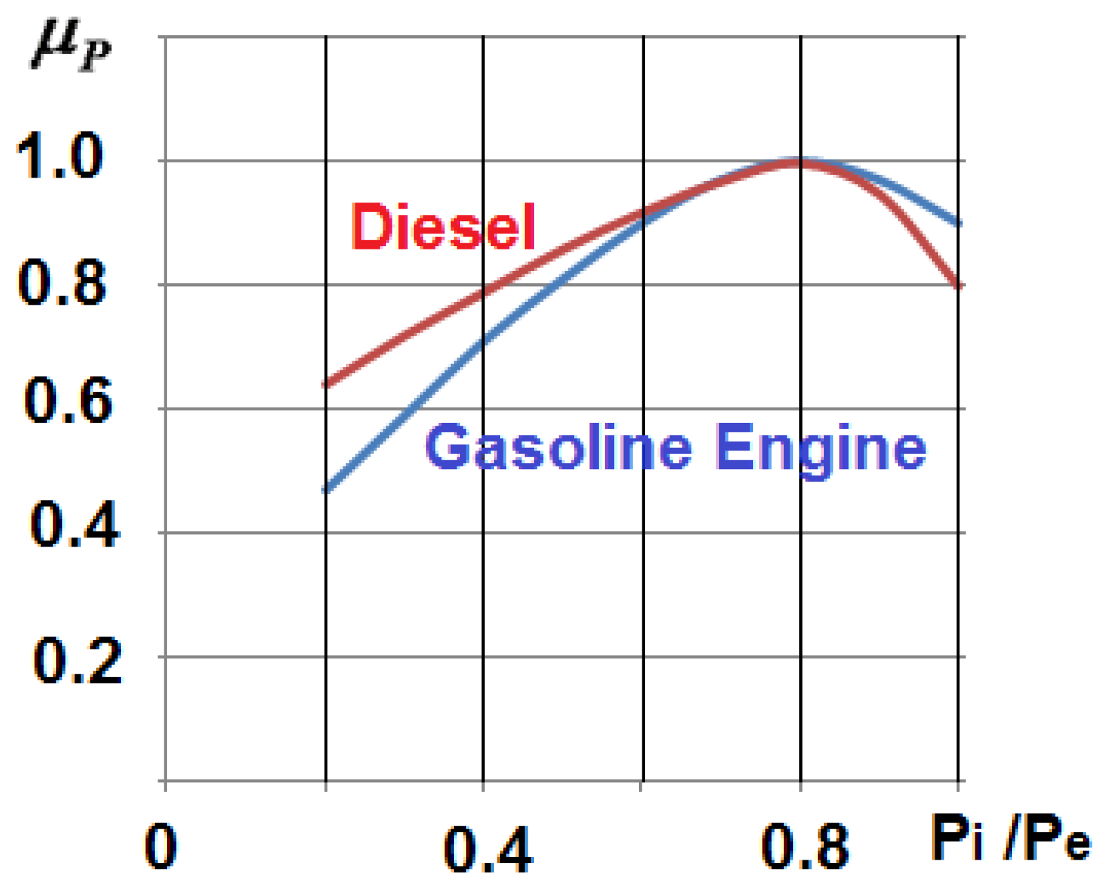
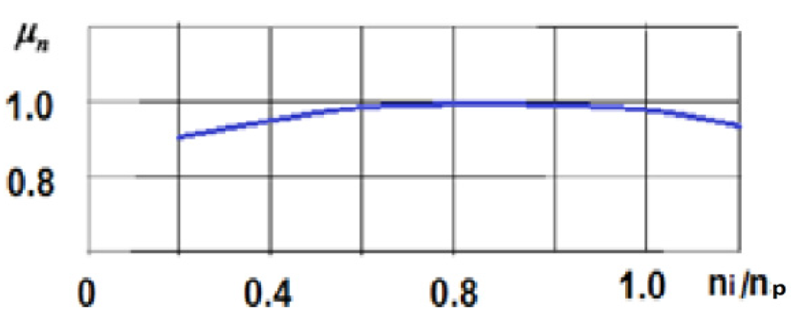
The above approach was used to carry out calculations of polynomials μ_P = f(P_i/P_e) and μ_n = f(n_i/n_p) for a number of modern car engines, whose characteristics were described in [15,16,17,18,19]. The results were then averaged and are shown in Figure 4 and Figure 5. It was revealed that for the majority of diesel and gasoline engines μ_P = 1 when P_i/P_e=0.8, and μ_n = 1 when n_i/n_p = 0.7 (see summary in Table 1).

Figure 4. Coefficient of the engine speed mode (same for diesel and gasoline engines).

Figure 4. Coefficient of the engine speed mode (same for diesel and gasoline engines).

Figure 5. Coefficient of the power utilization.

Figure 5. Coefficient of the power utilization.

Table 1. Coefficient values.

Pi/Pe, ni/np, %	μP, Gasoline	μP, Diesel	μn
0.20	0.47	0.64	0.87
0.30	0.59	0.72	0.92
0.40	0.71	0.79	0.96
0.50	0.82	0.89	0.98
0.60	0.90	0.92	0.99
0.70	0.97	0.97	1.00
0.80	1.00	1.00	0.99
0.90	0.97	0.95	0.98
1.00	0.90	0.80	0.96

Table 1. Coefficient values.

Pi/Pe, ni/np, %	μP, Gasoline	μP, Diesel	μn
0.20	0.47	0.64	0.87
0.30	0.59	0.72	0.92
0.40	0.71	0.79	0.96
0.50	0.82	0.89	0.98
0.60	0.90	0.92	0.99
0.70	0.97	0.97	1.00
0.80	1.00	1.00	0.99
0.90	0.97	0.95	0.98
1.00	0.90	0.80	0.96

The graphical relationships of Figure 3 and Figure 4 were further approximated by polynomials, and the following results were obtained. The relation for calculating μ_P for diesel engines is of the form:

$${\mu }_P=0.5968-0.1666\left(\frac{P_i}{P_e}\right)+2.4968{\left(\frac{P_i}{P_e}\right)}^2-2.1128{\left(\frac{P_i}{P_e}\right)}^3,$$

(7)

while μ_P for gasoline engines is calculated according to:

$${\mu }_P=0.234+1.0592\left(\frac{P_i}{P_e}\right)+0.8149{\left(\frac{P_i}{P_e}\right)}^2-1.2121{\left(\frac{P_i}{P_e}\right)}^3.$$

(8)

The formula for calculating μ_n for diesel and gasoline engines is obtained as:

$${\mu }_n=0.7107+0.9963\left(\frac{n_i}{n_P}\right)-1.0582{\left(\frac{n_i}{n_P}\right)}^2+0.3124{\left(\frac{n_i}{n_P}\right)}^3,$$

(9)

Maximum attainable engine power at n_i may be determined empirically as [1]:

$$P_e=P_P\left[a\left(\frac{n_i}{n_P}\right)+b{\left(\frac{n_i}{n_P}\right)}^2-c{\left(\frac{n_i}{n_P}\right)}^3\right][\text{kW}],$$

(10)

where P_P is the engine rated power and a, b, c are engine (gasoline/diesel) specific constants. The instantaneous engine speed is proportional to the instantaneous velocity of the vehicle:

$$n_i(t)=\frac{9.55v(t){\xi }_{ax}{\xi }_n}{r_d},$$

(11)

with r_d the rolling radius of the tire, m; ξ_ax the final drive gear ratio; ξ_n the gearbox gear ratio.

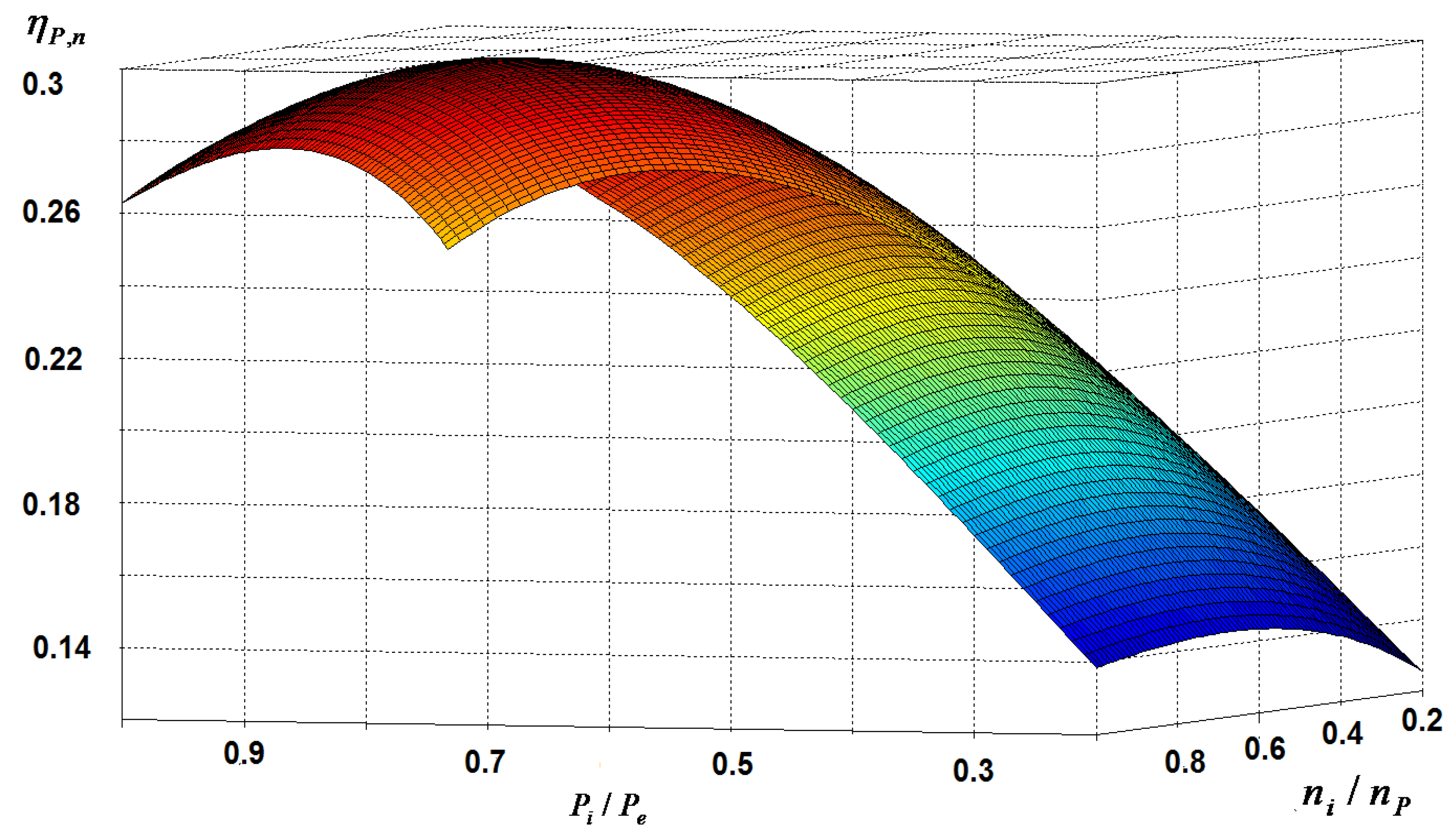
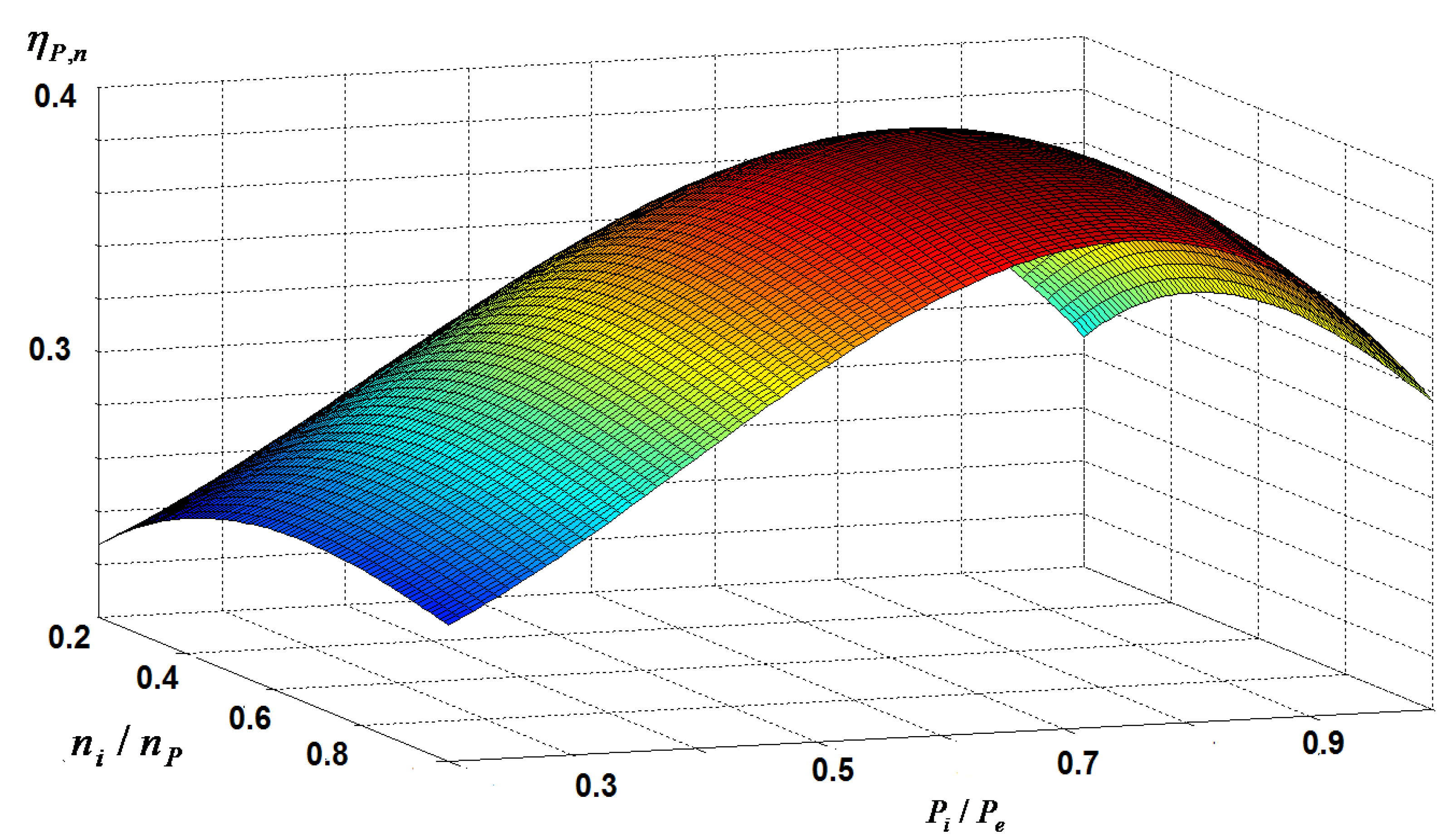
The resulting gasoline and diesel engine efficiencies are shown in Figure 6 and Figure 7, respectively, demonstrating the power and speed dependencies.

The instantaneous engine power is determined from the overall resistance forces as:

$$P_i=\frac{1}{{\eta }_T}\left(m_v\cdot g\cdot f_r\cdot \frac{v(t)}{3.6}+0.5\cdot {\rho }_a\cdot C_D\cdot A_f\cdot {\left\{\frac{v(t)}{3.6}\right\}}^3+m_v\cdot {\gamma }_m\cdot a(t)\right)$$

(12)

and fuel consumption per 100 km is given by:

$$Q_S=\frac{E_s}{H_L}\text{=}\frac{E_1+E_2}{H_L}[\text{l/100 km}]$$

(13)

where H_L is the calorific value of one liter of fuel, J∙L⁻¹.

Figure 6. Gasoline engines efficiency.

Figure 6. Gasoline engines efficiency.

Figure 7. Diesel engines efficiency.

Figure 7. Diesel engines efficiency.

3. Experimental Verification of the Derived Equations

To assess the validity and examine the feasibility of the obtained formulas, calculations of fuel consumption were carried out using the derived expressions and compared to experimental data available from manufacturers [19]. In order to carry out the required calculations, common peak efficiencies η_o where assumed as 0.4 for diesel engines and 0.3 for gasoline engines. The efficiency of the transmission η_T was taken as 0.95 for both (see Table 2). The results of the comparison are given in Table 3. The vehicle-specific parameters used were the type of engine, automobile mass, rated power and engine speed.

Table 2. The values of common parameters used in our calculations.

Engine	ηe	ηT
Diesel	0.40	0.95
Gasoline	0.30	0.95

Table 2. The values of common parameters used in our calculations.

Engine	ηe	ηT
Diesel	0.40	0.95
Gasoline	0.30	0.95

Table 3. Comparison results of vehicles fuel consumption.

Vehicle	Fuel consumption (technical specifications)		Fuel consumption (calculated)		Vehicle parameters
	Cycle		Cycle		Mass, kg	Rated power, kW	Rated speed, rpm
	EUDCE	URBAN	EUDCE	URBAN
Volkswagen Polo Sedan	4.8	7.7	4.9	7.4	1106	62.6	5000
Toyota Yaris	4.5	6.8	4.8	6.4	1005	73.1	6000
Toyota Sienna AWD	10.7	14.7	11.2	15.5	2080	197.6	6000
Toyota Camry AWD3.5	6.8	10.6	7.3	10.7	1570	196.9	6000
Hyundai Genesis Coupé 2.0 T	7.1	10.2	7.5	10.8	1570	157.3	6000
BMW 1-Series Convertible	8.4	13.0	8.7	12.5	1400	170	6500

Table 3. Comparison results of vehicles fuel consumption.

Vehicle	Fuel consumption (technical specifications)		Fuel consumption (calculated)		Vehicle parameters
	Cycle		Cycle		Mass, kg	Rated power, kW	Rated speed, rpm
	EUDCE	URBAN	EUDCE	URBAN
Volkswagen Polo Sedan	4.8	7.7	4.9	7.4	1106	62.6	5000
Toyota Yaris	4.5	6.8	4.8	6.4	1005	73.1	6000
Toyota Sienna AWD	10.7	14.7	11.2	15.5	2080	197.6	6000
Toyota Camry AWD3.5	6.8	10.6	7.3	10.7	1570	196.9	6000
Hyundai Genesis Coupé 2.0 T	7.1	10.2	7.5	10.8	1570	157.3	6000
BMW 1-Series Convertible	8.4	13.0	8.7	12.5	1400	170	6500

As shown by Table 3, the disagreement between the results of calculations and the experimental data is in the 2%–7% range, indicating that the obtained formula provides a sufficiently good approximation.

4. Effect of Design Parameters Variations on Fuel Consumption

In order to examine the sensitivity of fuel consumption to various parameter changes, the derived expressions were utilized with ECE urban driving cycle. The obtained sensitivity coefficients are summarized in Table 4 together with nominal parameter values. The obtained results are in close agreement with the sensitivity coefficients available in the literature.

Table 4. Sensitivity coefficients of fuel consumption to various design parameters.

Parameter	Diesel nominal value	Diesel sensitivity coefficient	Gasoline nominal value	Gasoline sensitivity coefficient
ma, kg	1000	0.13	1000	0.53
ηe	0.40	1.3	0.30	0.80
ηT	0.95	0.31	0.95	0.21
PP, kW	100	0.8	100	0.12
nP, min−1	5000	0.72	6000	0.34
ζax	3.5	0.05	3.5	0.03
ζn	1.0	0.071	1.0	0.06
rd, m	0.3	0.08	0.3	0.055
cr	0.015	0.14	0.015	0.25
Va, km/h	62.2	0.19	62.2	0.06
(ρ/2)cD, (N sec2)/m4	0.30	0.18	0.30	0.24
Af, m2	1.8	0.20	1.8	0.27
γm	1.08	0	1.08	0

Table 4. Sensitivity coefficients of fuel consumption to various design parameters.

Parameter	Diesel nominal value	Diesel sensitivity coefficient	Gasoline nominal value	Gasoline sensitivity coefficient
ma, kg	1000	0.13	1000	0.53
ηe	0.40	1.3	0.30	0.80
ηT	0.95	0.31	0.95	0.21
PP, kW	100	0.8	100	0.12
nP, min−1	5000	0.72	6000	0.34
ζax	3.5	0.05	3.5	0.03
ζn	1.0	0.071	1.0	0.06
rd, m	0.3	0.08	0.3	0.055
cr	0.015	0.14	0.015	0.25
Va, km/h	62.2	0.19	62.2	0.06
(ρ/2)cD, (N sec2)/m4	0.30	0.18	0.30	0.24
Af, m2	1.8	0.20	1.8	0.27
γm	1.08	0	1.08	0

5. Conclusions

In this paper, an analytical approach to evaluating vehicle fuel consumption under standard operating conditions was described. Vehicle fuel consumption was separated into two different operating modes: constant speed and acceleration movements. In each mode, the fuel consumption was shown to be dependent on the instantaneous engine efficiency, approximated using two analytical functions instead of a typically considered consumption map. The approximation was based on speed-power decoupling, allowing employing two single dimension polynomials instead of a two-dimensional lookup table.

Fuel consumption was determined under the assumption that the vehicle consumes fuel only when moving over a certain distance at a certain speed and when performing a series of accelerations on that same interval. Fuel consumption during decelerations and idle mode were not taken into account. This assumption was shown to have a negligible effect on the accuracy of the results for extra-urban driving modes. For urban conditions the accuracy of the results is somewhat lower. Equations taking into account fuel consumption at idle will be presented in a future work.

The adequacy and accuracy of the model was verified using comparison with experimental manufacturer-provided data. Moreover, the sensitivity of vehicle fuel consumption to various design parameters changes was derived utilizing the proposed model.

It would be of merit in a future work to introduce fuel economy enabling technologies into the analysis such as start-stop feature, mild hybrid or full hybrid to determine how to advance vehicle economy best.

References

- Froberg, A.; Nielsen, L. Efficient drive cycle simulation. IEEE Trans. Veh. Technol. 2008, 57, 1442–1453. [Google Scholar] [CrossRef]
- Wipke, K.; Cuddy, M.; Burch, S. Advisor 2.1: A user-friendly advanced powertrain simulation using a combined backward/forward approach. IEEE Trans. Veh. Technol. 1999, 48, 1751–1761. [Google Scholar] [CrossRef]
- Guzzella, L.; Sciarretta, A. Vehicle Propulsion Systems; Springer Verlag: Berlin, Germany, 2007. [Google Scholar]
- Gaevsky, V.; Ivanov, A. Theory of Ground Vehicles; MADI: Moscow, Russia, 2007. [Google Scholar]
- Kravets, V. Theory of Vehicles Handbook; University of Nizhni Novgorod, NNSU: Nizhni Novgorod, Russia, 2007. [Google Scholar]
- Ross, M. Fuel efficiency and the physics of automobiles. Contemp. Phys. 1997, 38, 3–10. [Google Scholar] [CrossRef]
- Ehsani, M.; Gao, Y.; Emadi, A. Modern Electric, Hybrid Electric and Fuel Cell Vehicles: Fundamentals, Theory and Design, 2nd ed.; CRC Press: Boca Raton, FL, USA, 2010. [Google Scholar]
- Tong, H.; Hung, W.; Cheung, C. On-road motor vehicle emissions and fuel consumption in urban driving conditions. J. Air Waste Manag. Assoc. 2000, 50, 543–554. [Google Scholar] [CrossRef] [PubMed]
- Widodo, S.; Hasegawa, T.; Tsugawa, S. Vehicle fuel consumption and emission estimation in environment-adaptive driving with or without inter-vehicle communications. In Proceedings of IEEE Intelligent Vehicles Symposium, Dearborn, MI, USA, 3–5 October 2000; pp. 382–386.
- Al-Momani, W.; Badran, O. Experimental investigation of factors affecting vehicle fuel consumption. Int. Jour. Mech. Mat. Eng. 2007, 2, 180–188. [Google Scholar]
- United Nations Economic Commission for Europe (UNECE). Vehicle Regulations. Available online: http://www.unece.org/trans/main/welcwp29.html (accessed on 1 August 2011).
- Wong, J.Y. Theory of Ground Vehicles; John Wiley and Sons: Ontario, Canada, 2000. [Google Scholar]
- Mitschke, M.; Wallwntowitz, H. Dynamik der Kraftfahrzeuge; Springer: Berlin, Germany, 2004. [Google Scholar]
- Bosch, R. Bosch Gasoline-Engine Management; Bentley Pub: Cambridge, MA, USA, 2004. [Google Scholar]
- Stone, R. Introduction to Internal Combustion Engines; Macmillan: Basingstoke, UK, 1985. [Google Scholar]
- Jimenez-Palacios, J. Understanding and Quantifying Motor Vehicle Emissions and vehicle Specific Power and Tildas Remote Sensing. Ph.D. Thesis, Massachusetts Institute of Technology, Cambridge, MA, USA, February 1999. [Google Scholar]
- Heywood, J. Internal Combustion Engine Fundamentals; McGraw-Hill, Inc.: New York, NY, USA, 1988. [Google Scholar]
- Ferguson, C.R.; Kirkpatrick, A.T. Internal Combustion Engine: Applied Thermosciences, 2nd ed.; John Wiley and Sons: New York, NY, USA, 2001. [Google Scholar]
- Speed Kills: Testing MPH vs. MPG in Top Gear. Available online: http://www.metrompg.com/posts/speed-vs-mpg.htm (accessed on 2 August 2006).
© 2013 by the authors; licensee MDPI, Basel, Switzerland. This article is an open access article distributed under the terms and conditions of the Creative Commons Attribution license (http://creativecommons.org/licenses/by/3.0/).
Share and Cite
MDPI and ACS Style
Ben-Chaim, M.; Shmerling, E.; Kuperman, A. Analytic Modeling of Vehicle Fuel Consumption. Energies 2013, 6, 117-127. https://doi.org/10.3390/en6010117
AMA Style
Ben-Chaim M, Shmerling E, Kuperman A. Analytic Modeling of Vehicle Fuel Consumption. Energies. 2013; 6(1):117-127. https://doi.org/10.3390/en6010117
Chicago/Turabian StyleBen-Chaim, Michael, Efraim Shmerling, and Alon Kuperman. 2013. "Analytic Modeling of Vehicle Fuel Consumption" Energies 6, no. 1: 117-127. https://doi.org/10.3390/en6010117