Article

Dynamic Output Feedback Power-Level Control for the MHTGR Based On Iterative Damping Assignment

Institute of Nuclear and New Energy Technology, Tsinghua University, Beijing 100084, China
Energies 2012, 5(6), 1782-1815; https://doi.org/10.3390/en5061782
Submission received: 26 April 2012 / Revised: 5 June 2012 / Accepted: 7 June 2012 / Published: 13 June 2012
(This article belongs to the Special Issue Electrical Power and Energy Systems)

Abstract

:
Because of its strong inherent safety features and high outlet temperature, the modular high temperature gas-cooled nuclear reactor (MHTGR) is already seen as the central part of the next generation of nuclear plants. Such power plants are being considered for industrial applications with a wide range of power levels, and thus power-level control is an important technique for their efficient and stable operation. Stimulated by the high regulation performance provided by nonlinear controllers, a novel dynamic output-feedback nonlinear power-level regulator is developed in this paper based on the technique of iterative damping assignment (IDA). This control strategy can provide the L2 disturbance attenuation performance under modeling uncertainty or exterior disturbance, and can also guarantee the globally asymptotic closed-loop stability without uncertainty and disturbance. This newly built control strategy is then applied to the power-level regulation of the HTR-PM plant, and numerical simulation results show both the feasibility and high performance of this newly-built control strategy. Furthermore, the relationship between the values of the parameters and the performance of this controller is not only illustrated numerically but also analyzed theoretically.

1. Introduction

After the severe nuclear accident at Fukushima, the safety issues of nuclear reactors have become much more significant than before. Because of its inherent safety characteristic and economic competitive power, the modular high-temperature gas-cooled reactor (MHTGR) is seen as the central part of the next generation nuclear plant (NGNP). MHTGRs use helium as coolant and graphite as both moderator and structural material, and its fuel elements contain thousands of very small coated particles that are embedded in a graphite matrix. The coatings surrounding the particle kernel produce a robust fuel form by acting as the containment boundary for radioactive material. The crucial inherent safety feature is guaranteed by the low power density and the slim shape of the reactor core [1,2,3], which makes the MHTGR meet and exceed current nuclear standards in reliability, waste management and safety. Moreover, the MHTGR can provide heat for industrial process at temperatures from 700 to 950 °C, which opens a door for a wider range of commercial applications than that of current light water reactors operating near 300 °C. Study on the MHTGR technology began in China at the end of the 1970s. A 10 MWth pebble-bed high temperature gas-cooled test reactor (HTR-10), which was built at Institute of Nuclear and New Energy Technology (INET) of Tsinghua University [4], achieved its criticality in December 2000 and full power level in January 2003. Six safety demonstration tests have also been done on the HTR-10, which have manifested both the inherent safety feature and the self-stabilizing features [5].
Figure 1. Schematic structure of the HTR-PM power plant.
Energies 05 01782 g001
Based upon the HTR-10, a high temperature gas-cooled reactor pebble-bed module (HTR-PM) project has then been proposed [6,7]. The HTR-PM plant consists of two pebble-bed one-zone module reactors of combined 2 × 250 MWth power, and adopts the operation scheme of two modules connected to one steam turbine/generator set. Here, the module is a nuclear steam supplying system (NSSS) composed of an MHTGR, a helical coiled once-through steam generator (OTSG) and some connecting pipes. The MHTGR and OTSG of one NSSS are arranged side by side and housed in independent steel pressure vessels, and the schematic view of the HTR-PM plant is illustrated in Figure 1.
It is exceedingly clear that safe, stable and efficient operation is a key requirement for the various industrial applications of the MHTGR power plants such as electricity production, process heat sources, etc. Power-level regulation is just one of the most significant techniques guaranteeing economic and stable control performance and is very meaningful for the operation of the MHTGR. The basic principle of the power-level control is generating the insertion and withdrawal speed signal of the control rods to regulate the plant power according to a demand signal based upon the measurement of the neutron concentration, coolant temperature, control rod positions, etc. Though the classical output feedback power-level control still dominates commercial nuclear power plant operation, due to the development of the current high speed industrial microprocessors, it is possible now to implement more modern control strategies for improving regulation performance, which has led to the development of a series of promising power-level controllers during the past two decades. Combining the features of both the static output feedback and the state feedback, Edwards et al. [8] developed the state feedback assisted classical controller (SFAC) which utilizes the state-feedback to modify the demand signal for an embedded classical output feedback controller, and is quite useful for the existing power plant implementation since it leaves the current classical feedback loop in place. In order for strengthening the robustness of the SFAC, the linear quadratic Gaussian regulation with loop transfer recovery (LQG/LTR) technique is then applied under the SFAC configuration [9,10]. Since the SFAC are essentially linear regulators which guarantees closed-loop stability only near the operating point, it is not suitable for those nuclear plants that should tightly follow the demand signal. Therefore, it is necessary to develop a nonlinear power-level controller with load-following ability. One way to design the nonlinear power-level control is based upon the system model. For example, Shtessel [11] designed a nonlinear power-level control strategy composed of a static state feedback sliding mode controller and a sliding mode state-observer for the TOPAZ II space nuclear reactor. The other way is to use the soft-computing methods such as the artificial neural network [12], fuzzy set [13,14] and genetic algorithm [15]. However, the performances of these intelligent controllers are usually determined by their training samples which are very expensive or not possible to be obtained. The theory of nonlinear power-level control of nuclear reactors is still under development, and there is still no mature controller design approach.
Generalized Hamiltonian system (GHS) theory is a promising control design method for nonlinear systems, whose basic idea is adding dissipative terms to a given dynamic system through feedback in order for the asymptotic closed-loop stability [16]. Both the energy shaping (ES) [17] and the interconnection and damping assignment passivity based control (IDA-PBC) [18] are effective GHS approaches which have been already applied to those mechanical [19], electromechanical [20] and power systems [21,22,23]. However, these two methods usually result in solving a set of complicated partial differential equations, which limits their application to the complex process systems such as the nuclear reactors. Stimulated by this and the need of designing nonlinear power-level regulation strategy for the MHT-GRs, a novel dynamic output-feedback power-level controller based on iterative damping assignment (IDA-PLC) is presented for the MHTGRs in this paper. The IDA-PLC is composed of a nonlinear state-feedback power-level regulator and a state observer. The regulator is realized by adding damping terms iteratively through state-feedback, and the observer just adopts the well-built dissipation based high-gain filter (DHGF) [24,25]. The IDA-PLC is an L2 disturbance attenuator when there exist exterior disturbances or modeling uncertainties, and it guarantees the globally asymptotic closed-loop stability if there is no disturbance and uncertainty. The IDA-PLC is then applied to the power-level control of the NSSS of the HTR-PM plant, and numerical simulation results show not only the feasibility of this newly-built MHTGR power-level control strategy but also the relationship between its performance and its parameters.
The rest part of this paper is organized as follows: both the nonlinear state-space model and the problem formulation are given in Section 2. Section 3 presents the iterative design of the state-feedback power-level regulator. In Section 4, the DHGF is applied to the state-observation of the MHTGR, and the performance of the entire dynamic output-feedback power control strategy formed by both the state feedback regulator and the observer is analyzed theoretically. Simulation results with discussion will be given in Section 5, and some conclusions are drawn in Section 6.

2. Nonlinear State-Space Model and Problem Formulation

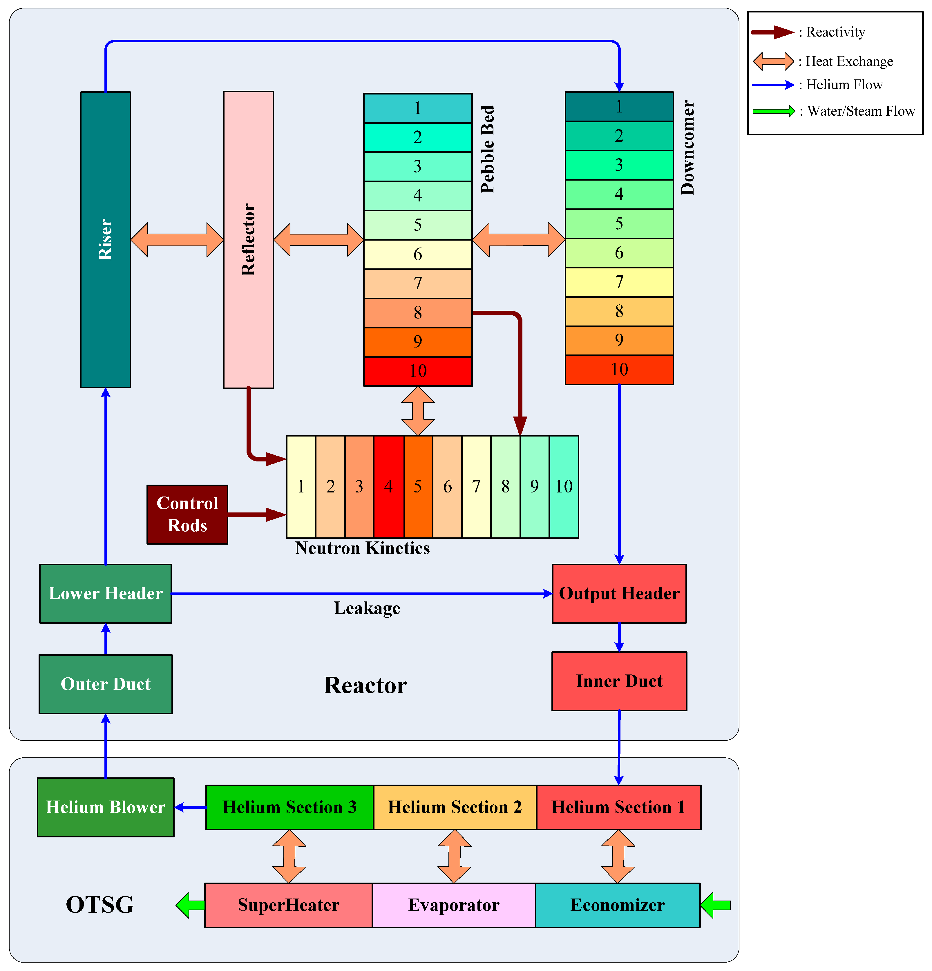
2.1. Nonlinear State-Space Model

The dynamic model of the MHTGR can be written as [26,27]:
Energies 05 01782 i001
where nr is the relative nuclear power; cr is the relative concentration of delayed neutron precursor; β is the fraction of delayed fission neutrons; Λ is the effective prompt neutron life time; ρr is the reactivity provided by the control rods; λ is the effective radioactive decay constant of the delayed neutron precursor; αc and αr are respectively the reactivity coefficients of the fuel and reflector temperatures; P0 is the rated reactor thermal power; Tc is the average fuel temperature; Td is the average temperature of the helium inside the pebble-bed; Td is the temperature of the helium entering into the pebble-bed; Tc,m and Td,m are initial equilibrium values of Tc and Td respectively; Tr is the reflector temperature; Ωcd and Ωcr are respectively the heat transfer coefficient between the fuel and helium in the pebble-bed and that between the fuel and reflector inside the riser; Mp is the mass flowrate times the heat capacity of the helium inside the primary loop; μc and μd are respectively the total heat capacities of the fuel or helium inside the pebble-bed; Gr is the differential reactivity worth of the control rod, and zr is the rod speed signal generated by the corresponding power-level control strategy.
To obtain the state-space model for power-level control design, the deviations of the actual values of nr, cr, Tc, Td, Tdin, Tr and ρr from their equilibrium values, i.e., nr0, cr0, Tc0, Td0, Tdin0, Tr0 and ρr0 are respectively defined as:
Energies 05 01782 i002
Moreover, we define:
Energies 05 01782 i003
Energies 05 01782 i004
and:
Energies 05 01782 i005
Then, the nonlinear state-space model for power-level control design can be written as:
Energies 05 01782 i006
where:
Energies 05 01782 i007
Energies 05 01782 i008
Energies 05 01782 i009
and:
Energies 05 01782 i010
It is noted that the heat capacity of the reflector of the MHTGR is so large that δTr changes very slowly and its amplitude is also very small. Moreover, δTdin reflects the influence of the other parts of the MHTGR to the reactor core dynamics. Therefore, it is quite reasonable to view w defined in Equation (4) as the disturbance.

2.2. Problem Formulation

Here, define the evaluation signal of System (6) as:
Energies 05 01782 i011
where the vector-valued function ζ is smooth. Then the concept of L2 disturbance attenuator is introduced as follows:
Definition 1 [15]: consider nonlinear System (6) with evaluation Signal (11). Control input u is said to be an L2 disturbance attenuator if there is a semi-positive smooth function V(x) such that following γ-dissipation inequality is satisfied:
Energies 05 01782 i012
where Q(x) is a semi-positive function; ||·||2 is the Euclidean norm, and here γ is a positive scalar called the L2 gain from disturbance w to evaluation signal ζ.
Remark 1: from Inequality (12), when wO:
Energies 05 01782 i013
Based upon Inequality (13), it is clear that if ∀x ∈ Γ = {x | V (x) ≡ 0} satisfies x→0 as t→∞, then from Lasalle’s invariance principle, the system is asymptotic stable. After introducing the concept of L2-disturbance attenuator, the problem to be solved in this paper is given as follows:
Problem 1: how to design an L2-disturbance attenuator for System (6) with evaluation Signal (11)? That is to say, how to design a power-level controller for the MHTGR with L2-disturbance attenuation performance?

3. Power-Level Control Based on Iterative Damping Assignment

As we have discussed above, instead of the classical control design techniques that try to impose some predetermined dynamic behavior—usually through nonlinearity cancellation and high gain, the control design based on feedback dissipation is an ever increasing predominance of control techniques. However, the existing feedback dissipation approach such as energy shaping (ES), interconnection and damping assignment passivity based control (IDA-PBC) and etc. usually need System (6) to satisfy the following matching condition:
Energies 05 01782 i014
where H is a semi-positive function called Hamiltonian function. Moreover, the control design by the existing feedback dissipation approach certainly leads to solve a set of partial differential equations.
From Equations (8,10), the dimensions of vectors h and g imply that matching Condition (14) cannot be satisfied here. Furthermore, solving partial differential equations may also lead to intensive complexity. Thus, in this section, the damping assignment is performed by state-feedback iteratively. In the following, the concept of feedback dissipation is firstly introduced. The power-level control (PLC) is then designed through the approach of iterative damping assignment (IDA). Finally, the closed-loop stability and L2-disturbance attenuation performance of the IDA-PLC are both verified.

3.1. Introduction to the Concept of Feedback Dissipation Control

To introduce the concept of the feedback dissipation control, the concept of the dissipative system is firstly given as follows:
Definition 2: consider the following nonlinear autonomous system:
Energies 05 01782 i015
where χRn and ω(O) = O. If there exists a smooth function Γ(·): Rn→R+ = [0, ∞) called Hamiltonian function so that inequality is satisfied:
Energies 05 01782 i016
Then System (15) is said to be a dissipative system corresponding to Hamiltonian function Γ. Moreover, if Inequality (16) holds strictly, then System (15) is strictly dissipative. After introducing the dissipative system, the concept of the generalized Hamiltonian realization is given as follows:
Definition 3: System (15) is called to have a generalized Hamiltonian realization (GHR) if there is a suitable subsets of Rn such that System (15) can be expressed as:
Energies 05 01782 i017
where Energies 05 01782 i096,and TRn×n is called the structure matrix. Moreover, if structure matrix T can be written as:
Energies 05 01782 i018
with skew-symmetric J and symmetric nonnegative definite R.
Remark 2: if the structure matrix of System (15) can be represented as Equation (18), then it is dissipative. Moreover, if symmetric matrix R is strict positive definite, then System (15) is strict dissipative.
From Definition 2, system dissipation means shrinkage of a given Hamiltonian function. However, not all of the dynamic systems are dissipative for a given Hamiltonian function, it is reasonable to force a system to be dissipative by the means of feedback. This leads to the definition of feedback dissipation control given as follows:
Definition 4: consider the following nonlinear system:
Energies 05 01782 i019
where χRn is the system state vector; vRp is the control input; θRm is the system output, and ω(O) = O. For a given Hamiltonian function Γ(χ), feedback control υ is called a feedback dissipation control if Inequality (20) is satisfied:
Energies 05 01782 i020
If Inequality (20) is strictly satisfied, then υ is called a strict feedback dissipation control. If υ = υ(χ), then it is a state-feedback dissipation control. If υ = υ(θ), then it is called an output-feedback dissipation control. Finally, in order for the closed-loop stability analysis, the concepts of zero-state detectability and observability are introduced as follows:
Definition 5 [15]: consider nonlinear System (19), and System (19) is called zero-state detectable if θO and υO (∀t ≥ 0) implies:
Energies 05 01782 i021
Moreover, this system is called zero-state observable if θO and υO implies z(t) ≡ O for ∀t ≥ 0.

3.2. Design of the Power-Level Control Based on Iterative Damping Assignment

Firstly, we adopt the following the state transformation:
Energies 05 01782 i022
and then reactor Dynamics (6) can be rewritten as:
Energies 05 01782 i023
where:
Energies 05 01782 i024
Energies 05 01782 i025
Energies 05 01782 i026
and:
Energies 05 01782 i027
In the following, the iterative damping assignment for system (23) is done through state-feedback dissipation step by step:
Step 1:
Define:
Energies 05 01782 i028
and then reactor dynamics can be rewritten as:
Energies 05 01782 i029
where:
Energies 05 01782 i097
We can see from the first equation of Equation (29) that it already has the form like a GHR. Next, we shall do like this iteratively.
Step 2:
Based on coordinate Transformation (28), define:
Energies 05 01782 i030
where:
Energies 05 01782 i031
and:
Energies 05 01782 i032
From Equations (28,30), the reactor dynamics can be transformed to:
Energies 05 01782 i033
where:
Energies 05 01782 i098
Step 3:
Based on Equation (33), we choose the feedback control u as:
Energies 05 01782 i034
where:
Energies 05 01782 i035
Energies 05 01782 i036
Energies 05 01782 i037
where v is the compensation term to be designed for guaranteeing the dissipation or stability characteristics of the closed-loop system, and here both κ and σ are given positive scalars.
Substituting control law Equation (33) to Equation (34), we can obtain:
Energies 05 01782 i038
where:
Energies 05 01782 i039
Energies 05 01782 i040
Energies 05 01782 i041
Energies 05 01782 i042
Energies 05 01782 i043
Energies 05 01782 i044
Energies 05 01782 i045
From Equations (28,30), the coordinate transformation from z to ξ can be expressed as:
Energies 05 01782 i046
Moreover, from Equations (22,46), it is clear that the transformation from x to ξ is:
Energies 05 01782 i047
Under coordinate x, feedback law Equation (34) can be written as:
Energies 05 01782 i048
The following Proposition 1, which is the first main result of this paper, gives the condition so that feedback law Equation (34) is an L2 disturbance attenuator corresponding to a given evaluation signal.
Proposition 1: choose the evaluation signal as:
Energies 05 01782 i049
where ξ, H and p is determined by Equations (40,43,47), respectively. If the compensation term v satisfies:
Energies 05 01782 i050
where K is a given positive scalar, then feedback law composed of Equations (48,50) is an L2 disturbance attenuator corresponding to evaluation signal Equation (49). Moreover, the L2 gain can be adjusted by feedback gain K. Moreover, if there is no disturbance, i.e.:
Energies 05 01782 i051
then the closed-loop system is globally asymptotically stable.
Proof: based on the above discussion, it is so clear that differentiating Hamiltonian function Equation (40) along the trajectory given by Equations (6,48,50) is equivalent to that along the trajectory given by Equations (38,50). Then, we can derive that:
Energies 05 01782 i052
where:
Energies 05 01782 i053
From Equation (42) and Inequality (52), we can properly choose the values of κ and γ such that inequality is satisfied:
Energies 05 01782 i054
where τ is a small positive scalar. Based upon Inequalities (52,54), we have:
Energies 05 01782 i055
By the use of Inequality (55) and Definition 1, we can easily see that the feedback law composed of Equations (48,50) is an L2 attenuator of system Equation (6) corresponding to evaluation signal Equation (49). Moreover, from Inequality (55), the L2 gain from disturbance w to evaluation signal ζ is:
Energies 05 01782 i056
which means that the influence of w to ζ can be effectively reduced by choosing a large K or a large σ. In the following, we shall prove the globally asymptotic closed-loop stability when Condition (51) is satisfied. It is clear that if Equation (51) holds, we have:
Energies 05 01782 i057
where:
Energies 05 01782 i058
From Equations (40,57,58), state-vector x asymptotically converges to the set defined as:
Energies 05 01782 i059
Based upon coordinate Transformation (47), set Ξ is equivalent to:
Energies 05 01782 i060
Moreover, from Equations (6,7), for ∀xΞ1, it is quite clear that:
Energies 05 01782 i099
which manifests that the closed-loop system is globally asymptotically stable if wO. This completes the proof of this proposition.
Remark 3: based on Inequality (57) and Equation (58), when there is no disturbance, the closed-loop system is still globally asymptotically stable even if K = 0. That is to say, feedback law Equation (34) with v = 0 is enough to guarantee the globally asymptotic closed-loop stability in case of wO.
Remark 4: from Equations (40,43,47), it is easily to see that:
Energies 05 01782 i061
and:
Energies 05 01782 i062
Substituting Equation (48) to Equation (62), we can get the total feedback control law, i.e.,
Energies 05 01782 i063
where:
Energies 05 01782 i064
Energies 05 01782 i065
Energies 05 01782 i066
It can be easily seen from Equation (63) that the function of this control law is realized through feeding back all the state-variables. Since only x1 and x3, i.e., δnr and δTd can be obtained through measurement, it is quite necessary to design a convergent state-observer for the implementation of this newly-built power-level control strategy.

4. Dynamic Output-Feedback Power-Level Control Strategy

In this section, for the implementation of the nonlinear state-feedback power-level controller Equation (63), the corresponding state-observer is designed firstly. Based on this observation strategy, the dynamic output-feedback power-level control law is developed. Through theoretical analysis that will be given in this section, this control strategy can provide power-level regulation function for the MHTGR with the performance of L2 disturbance attenuation.

4.1. Observation Strategy

The dissipation-based high-gain filter (DHGF) is an asymptotic state-observer for nonlinear systems, which has been proved to satisfy the separation principle. The DHGF is firstly introduced in this sub-section, and then a DHGF is designed for MHTGR dynamics Equation (6) without disturbances.
Consider the following nonlinear dynamic system:
Energies 05 01782 i067
where ςRn is the state-vector; ηRm is the system output; μRp is the control input and vector-valued functions ψ, φ and χ are all smooth.
Suppose that the state-observer corresponding to System (67) takes the form as:
Energies 05 01782 i068
where Energies 05 01782 i100 is the state-observation, FoRn×m is the gain matrix of the observer,
Energies 05 01782 i069
and:
Energies 05 01782 i070
Moreover, we define the observation error as:
Energies 05 01782 i071
and then it is clear that the dynamics of the observation error can be written as:
Energies 05 01782 i072
where:
Energies 05 01782 i073
The following Lemma 1 guarantees not only the convergence of State-observer (68) but also the stability of the closed-loop system composed of Dynamics (67), a stabilizer μ and Observer (68):
Lemma 1 [24,25]: Consider nonlinear system Equation (67) with State-observer Equation (68), and here suppose that:
Energies 05 01782 i074
is a state-feedback control law for System (67). Moreover, assume that observation error dynamics Equation (72) with its output defined as Equation (69) is zero-state observable, and there exists a smooth function Θ O ( ) : R m R + [ 0 , + ) , which satisfies:
Energies 05 01782 i075
and is only minimal at point τ = O. Then state-observer Equation (68) is convergent and dynamic output feedback controller:
Energies 05 01782 i076
is also an asymptotic stabilizer if:
Energies 05 01782 i077
where ϑ is a small enough positive scalar. The State-observer (68) with its gain matrix satisfying Equation (77) is called the dissipation-based high gain filter (DHGF).
Proof: See References [24,25].

4.2. Design and Analysis of the Dynamic Output-Feedback Power-Level Control Strategy

From the above discussion, it is natural for us to design the state-observer for System (6) as:
Energies 05 01782 i078
where f(·) and g is respectively defined by Equations (7,8), output function h(·) is determined by Equation (10), and control law u(·) is given by Equation (63). Based on Equations (63,78), the corresponding dynamic output feed-back controller can be written as:
Energies 05 01782 i079
where functions f(·), g, h(·) and u(·) respectively have the same meaning with those in Equation (78). Moreover, it is clear that the corresponding observation error dynamics of Equation (78) is:
Energies 05 01782 i080
where:
Energies 05 01782 i081
Energies 05 01782 i082
and:
Energies 05 01782 i083
Following Proposition 2, which is the second main result in this paper, gives a sufficient condition for dynamic output feedback controller Equation (79) to be an L2 disturbance attenuator.
Proposition 2: dynamic output feedback controller Equation (79) is an L2 disturbance attenuator for System (6) if the gain matrix KO satisfies:
Energies 05 01782 i084
where:
Energies 05 01782 i085
where ε is a small enough positive scalar. Furthermore, if there is no disturbance, i.e., Condition (51) holds, then control strategy Equation (79) is a globally asymptotic stabilizer, and Observer (78) is also convergent.
Proof: Define:
Energies 05 01782 i086
and it is clear that function HO (·) is only minimal at eyO. It is also easily to derive that:
Energies 05 01782 i087
which means that Condition (75) is satisfied.
Substituting eyO and wO to observation error dynamics Equation (80), and we have:
Energies 05 01782 i088
which is equivalent to:
Energies 05 01782 i089
Since the value of x3 can be arbitrarily given, it is easily to see from Equation (89) that:
Energies 05 01782 i090
which means that observation error Dynamics (80) under Condition (51) is zero-state observable with its output defined as ey. Since state-feedback control Equation (48) is a globally asymptotic stabilizer if Condition (51) is satisfied, it can be seen from Lemma 1, Equations (86,87,90) that control strategy Equation (79) is still a globally asymptotical stabilizer and Observer (78) is convergent under Condition (51).
Next, we shall prove that control law Equation (79) is still an L2 disturbance attenuator even if wO. Define the extended Hamiltonian function for the closed-loop system composed of Equations (6,79) as:
Energies 05 01782 i091
where functions H(·) and HO(·) are determined by Equations (40,86), respectively. Differentiating Equation (91) along the trajectory given by Equations (6,79), we can derive that:
Energies 05 01782 i092
where matrices L and M are respectively defined by Equations (53,85).
From Inequality (92), by properly choosing the values of positive scalars κ, γ and ε, it is easy to guarantee that inequalities:
Energies 05 01782 i093
Energies 05 01782 i094
where θ1 and θ2 are both small positive scalars.
From Inequalities (92–94), we find that:
Energies 05 01782 i095
where θ =θ1 + θ2. Based upon Inequality (95) and Definition 1, it is now quite clear that dynamic output feedback control strategy Equation (79) with observer gain Equation (84) and a small enough ε is still a L2 disturbance attenuator in case of wO. This is completes the proof of Proposition 2.

5. Simulation Results with Discussion

To show the feasibility and performance of the dynamic output feedback power-level control law determined by Equations (7,8,10,63,79) this newly developed controller is applied to the power-level regulation of a NSSS of the HTR-PM plant in this section. The influence of the controller parameters to the control performance is also illustrated and analyzed.

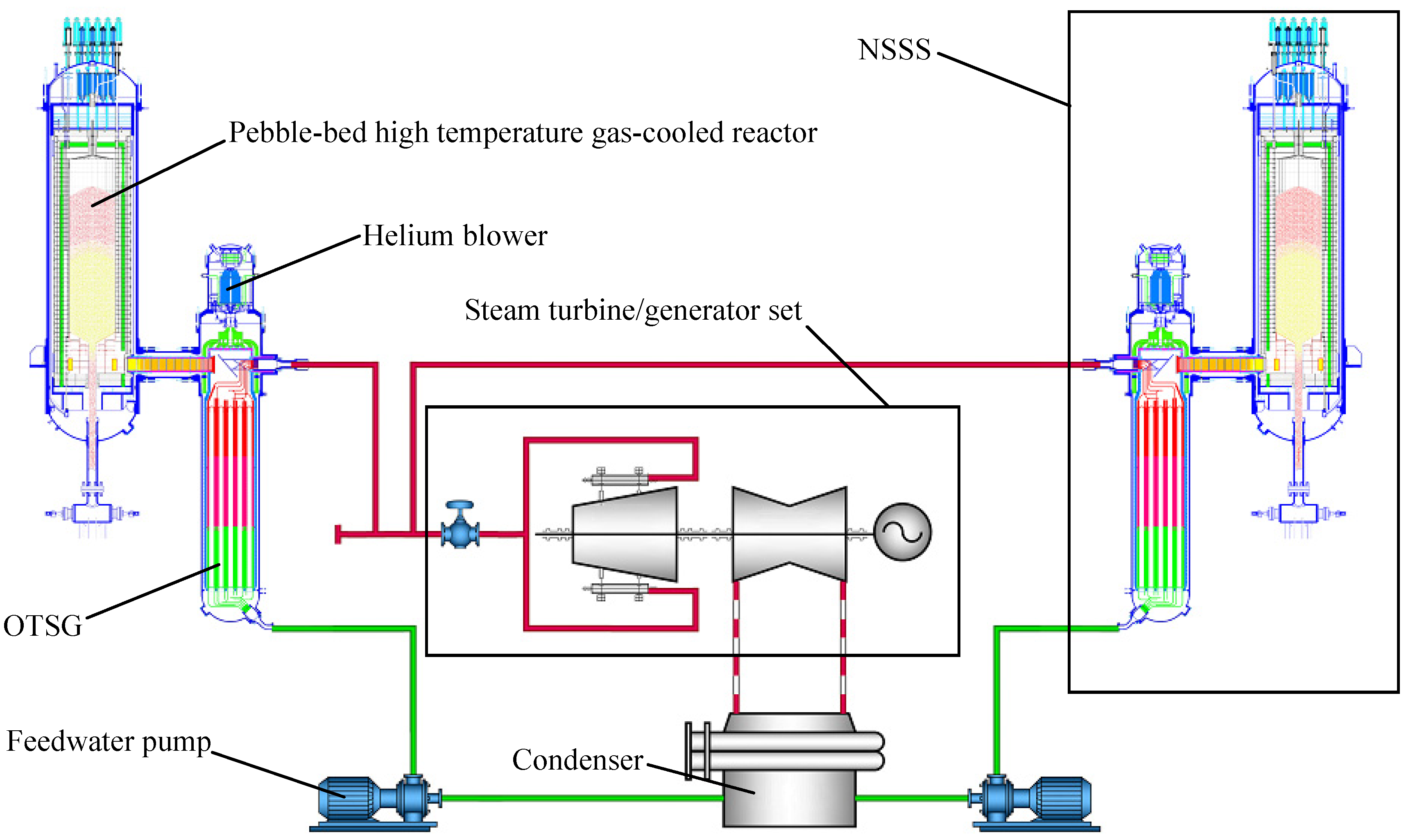
5.1. Description of the Numerical Simulation

The numerical simulation model is developed based on Visual C++. Since the height-to-diameter ratio of the HTR-PM reactor is nearly 4, the classical point kinetics model is not suitable for building the simulation code of the reactor core. By dividing the active core region into 10 parts vertically, a nodal neutron kinetics model and its thermal-hydraulic model are utilized to establish the simulation code [27]. The adopted OTSG model is just the classical moving boundary model [28]. The schematic view of the dynamic model of the NSSS for numerical simulation is shown in Figure 2. Furthermore, the model of the steam turbine and that of the electrical generator are also included in the simulation code [29]. The numerical simulation of this paper was done by the use of this simulation code.
Figure 2. Schematic view of the dynamic model of the NSSS.
Energies 05 01782 g002

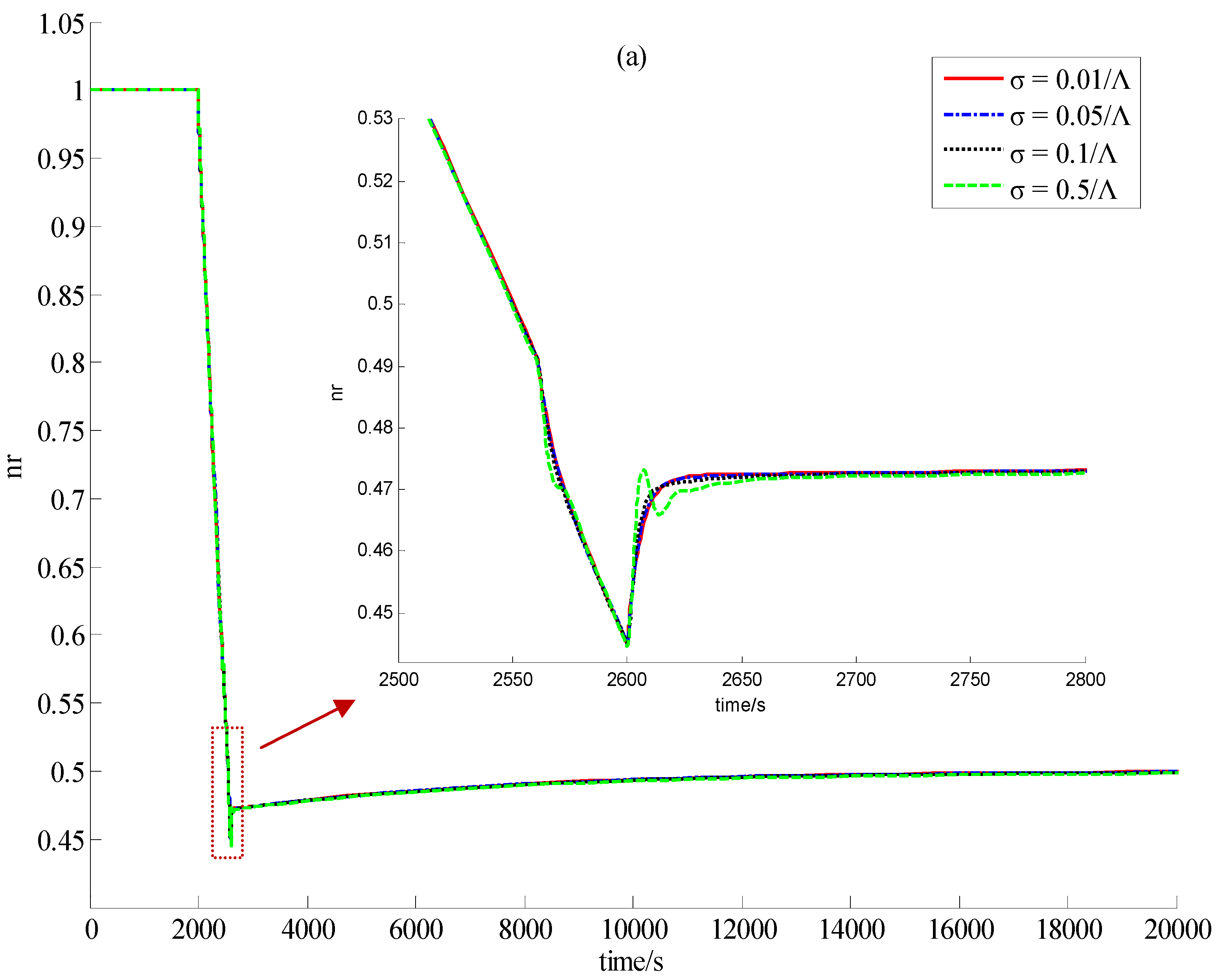
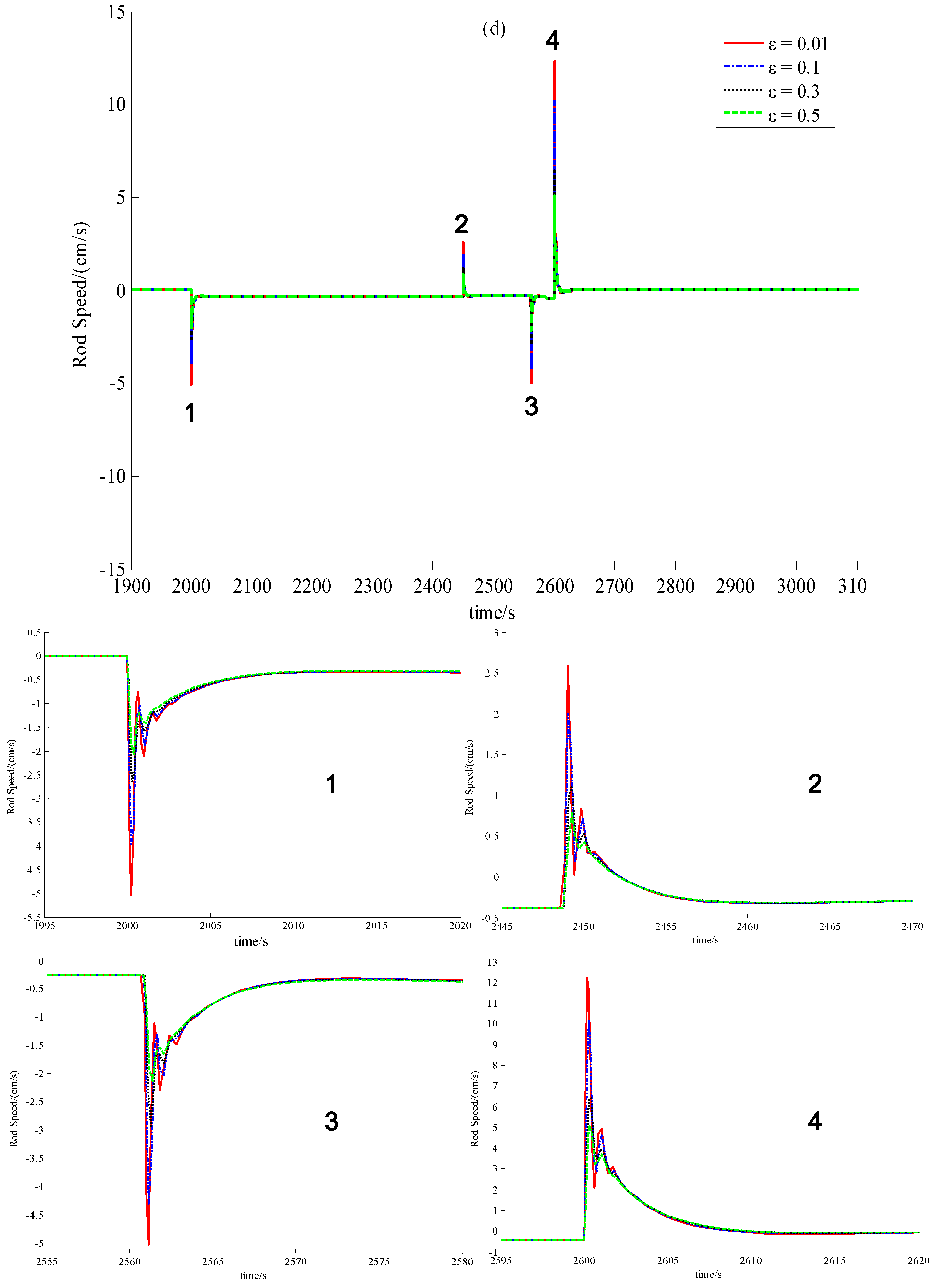
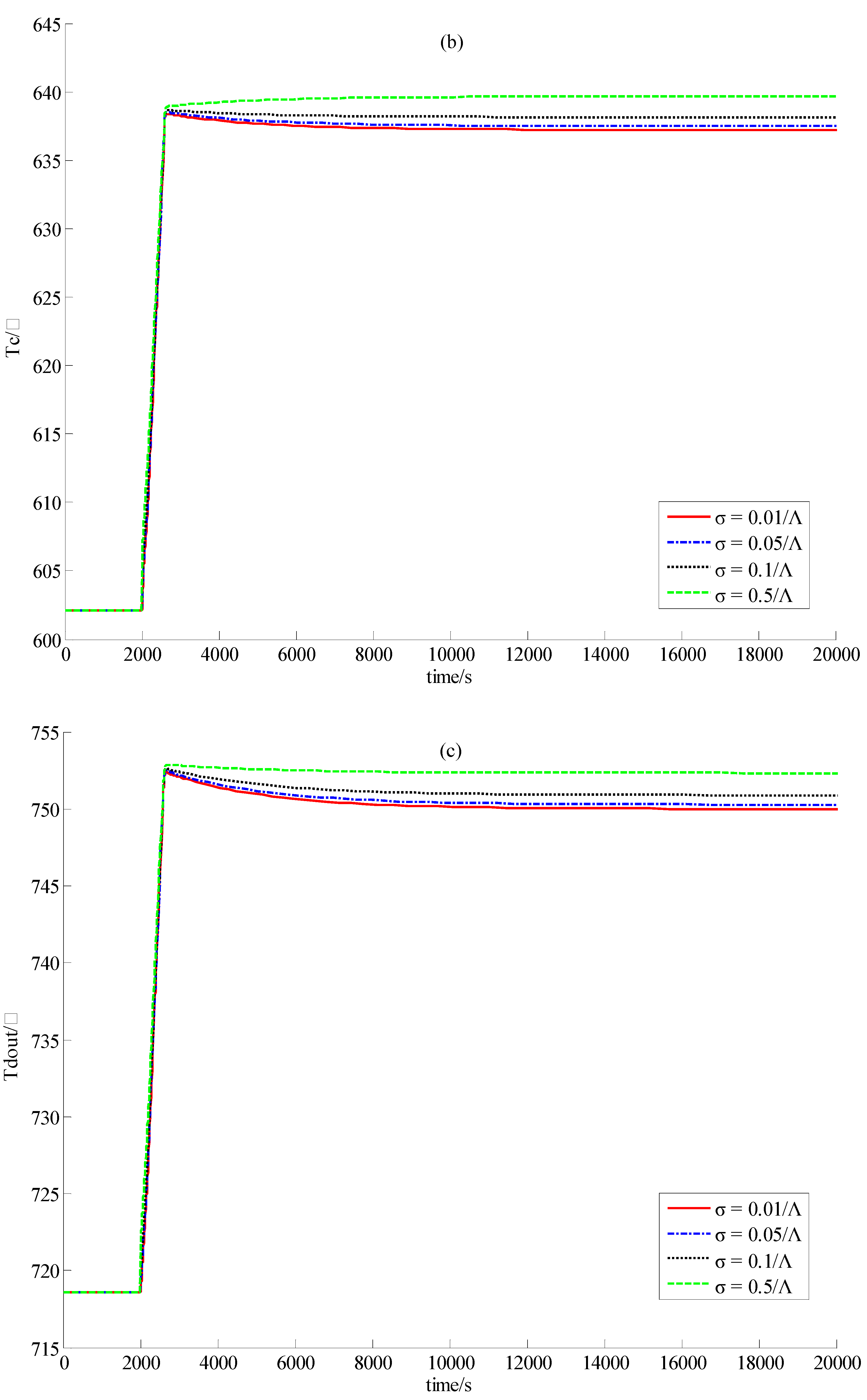
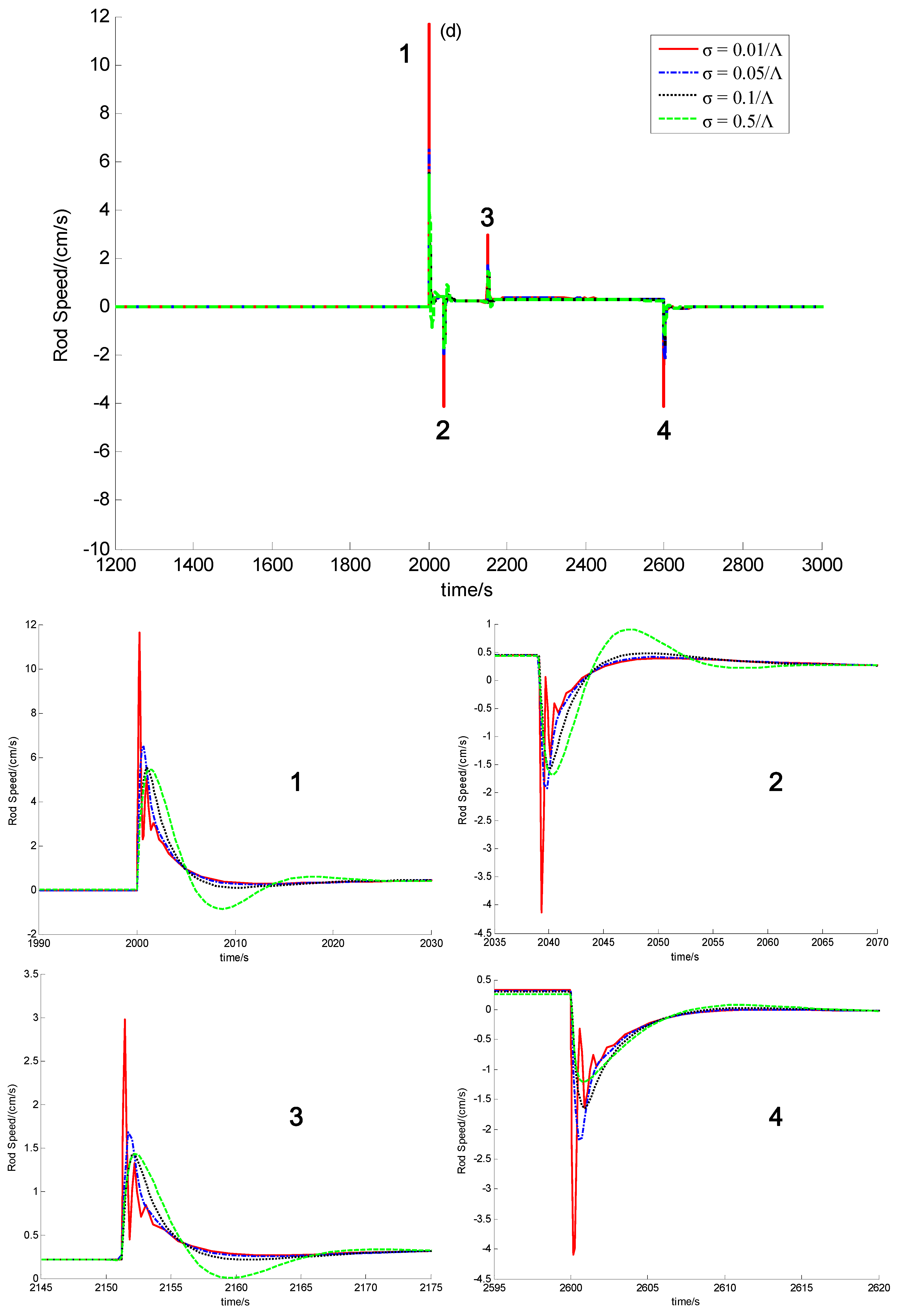
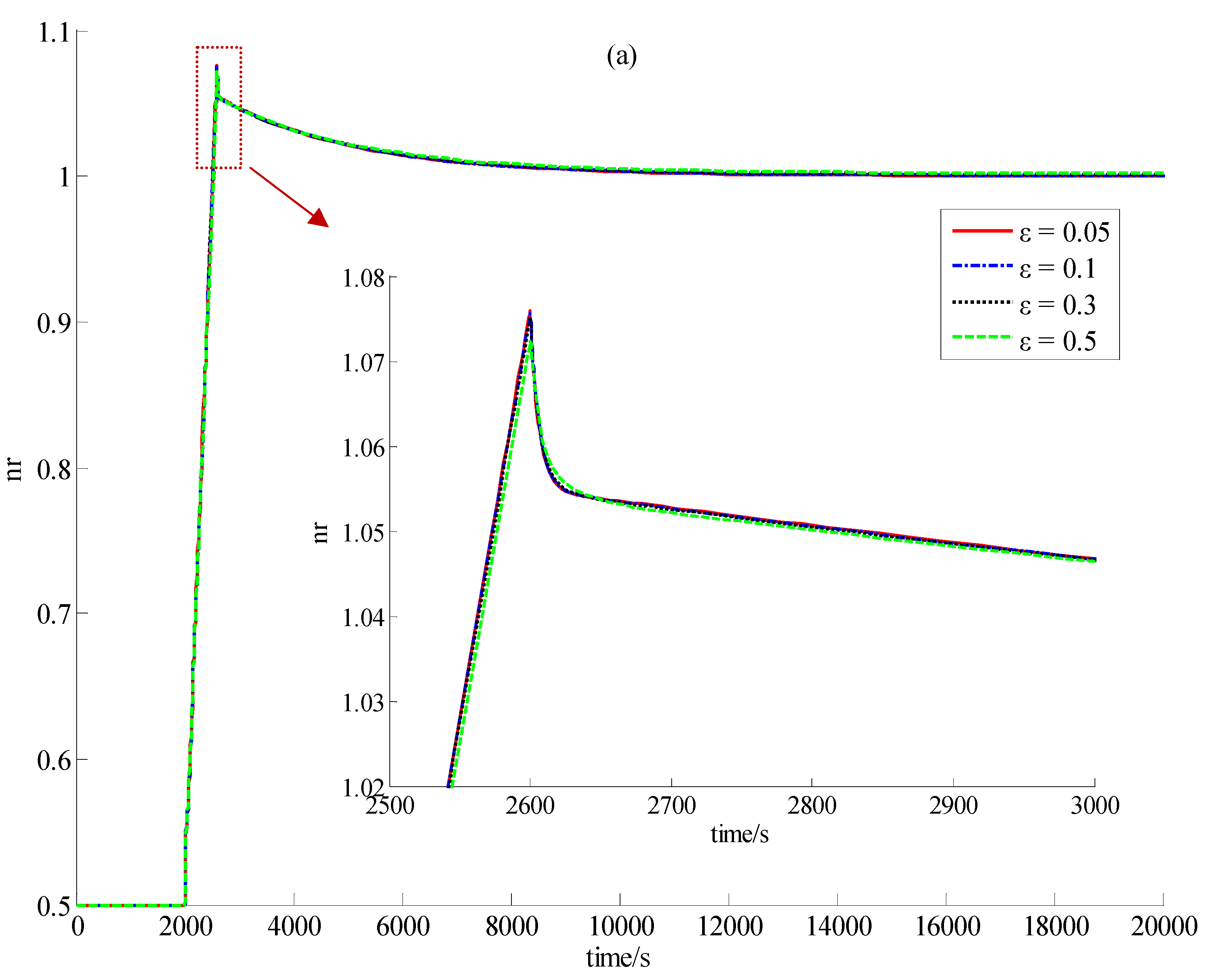
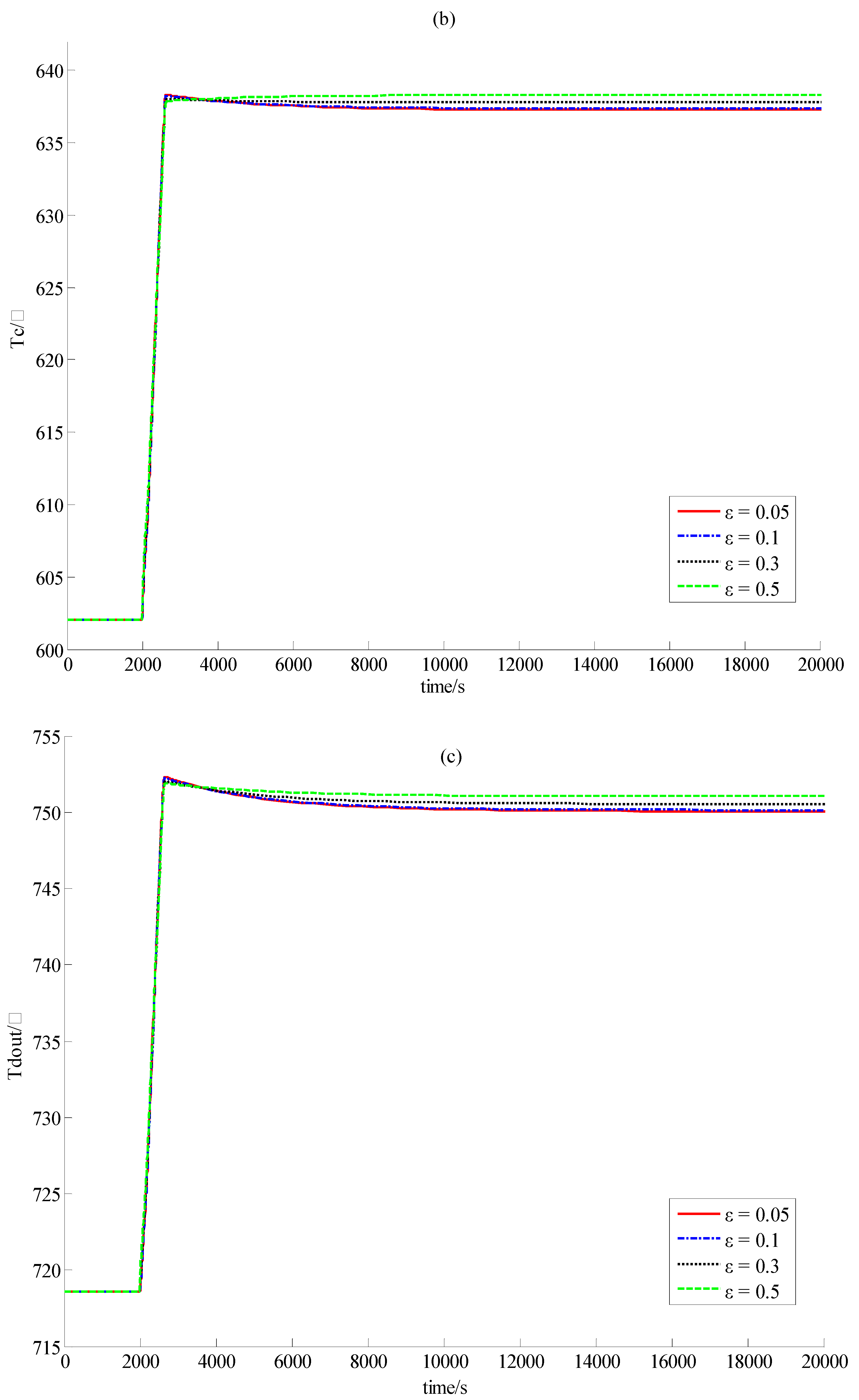
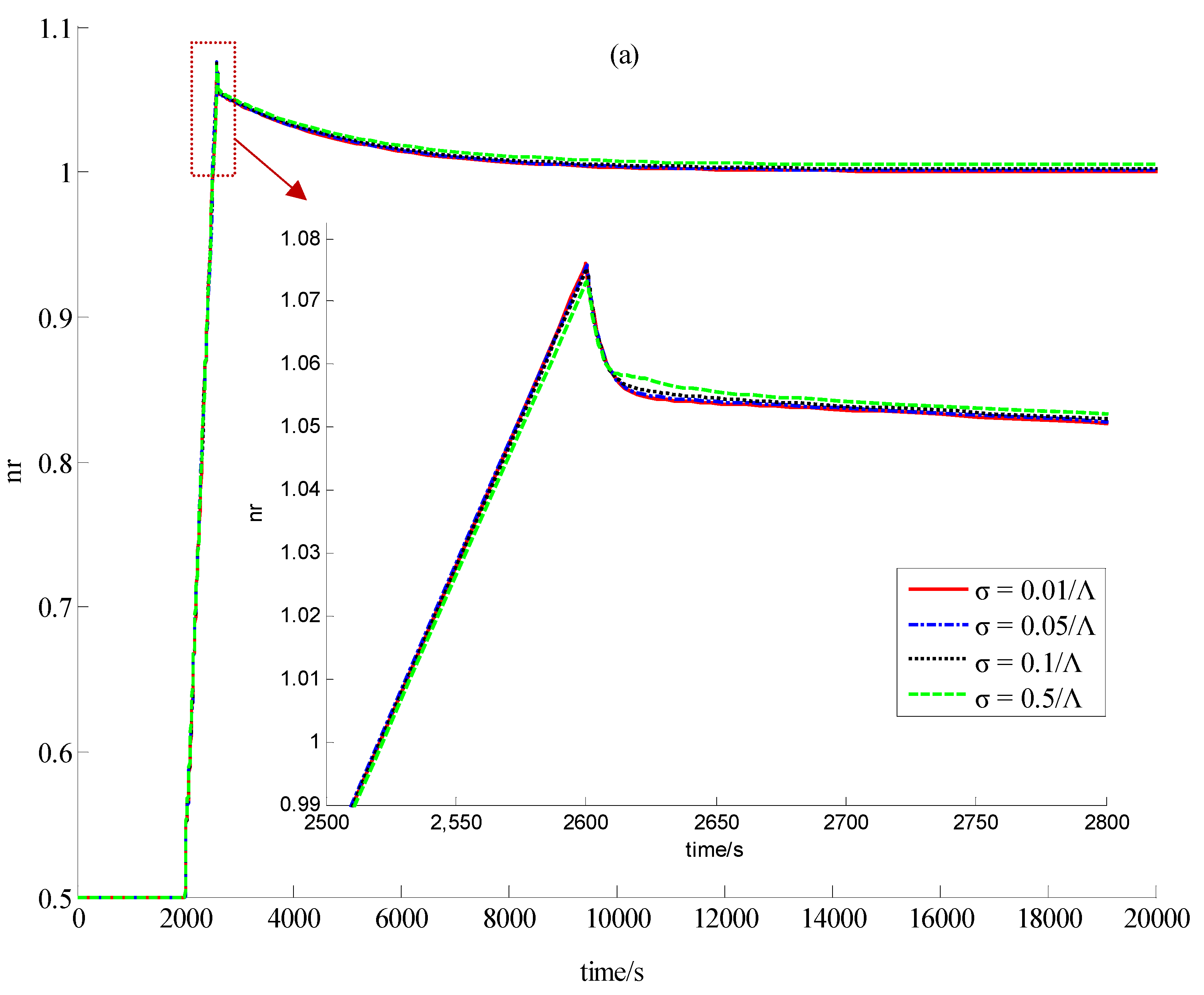
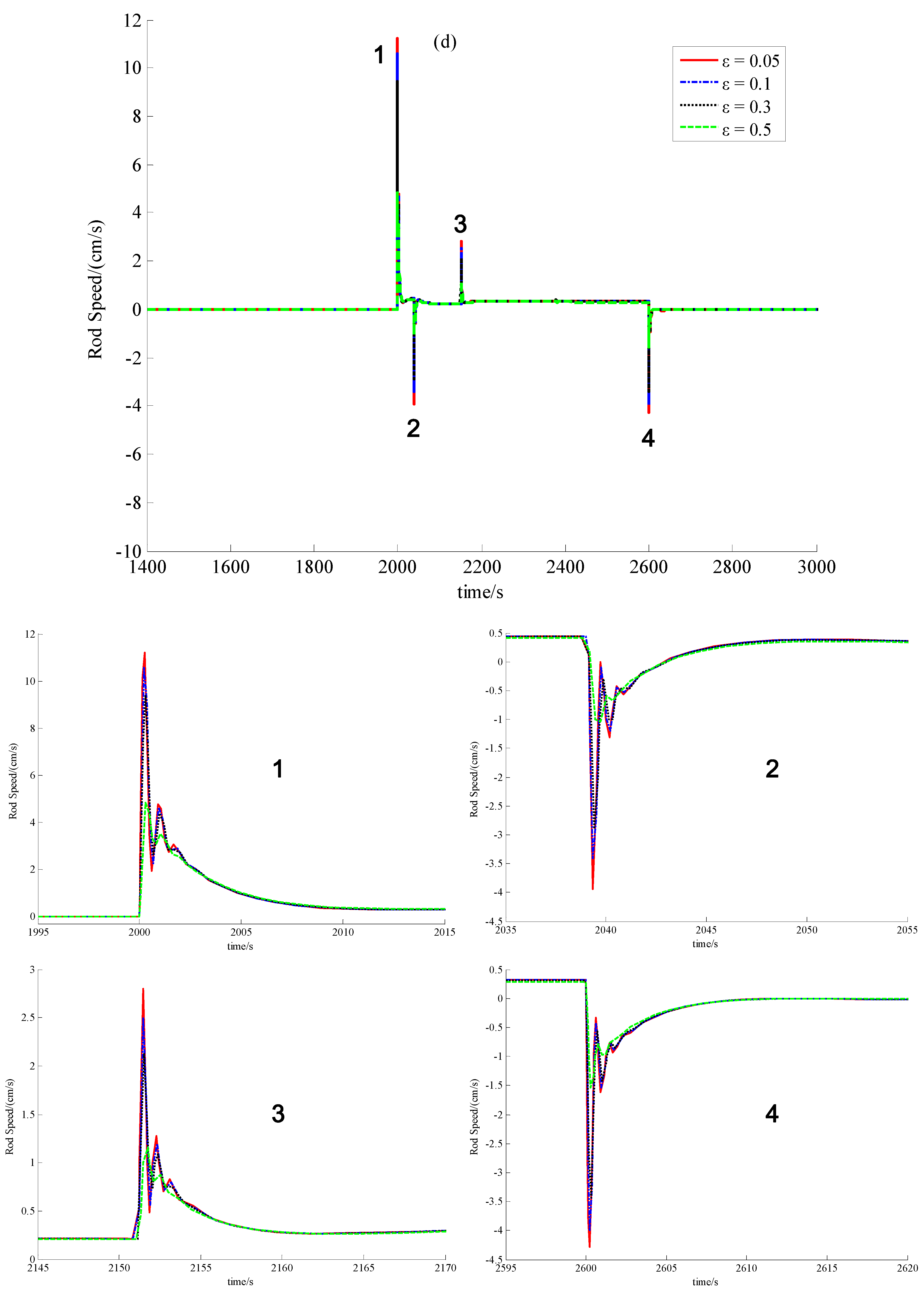
5.2. Simulation Results
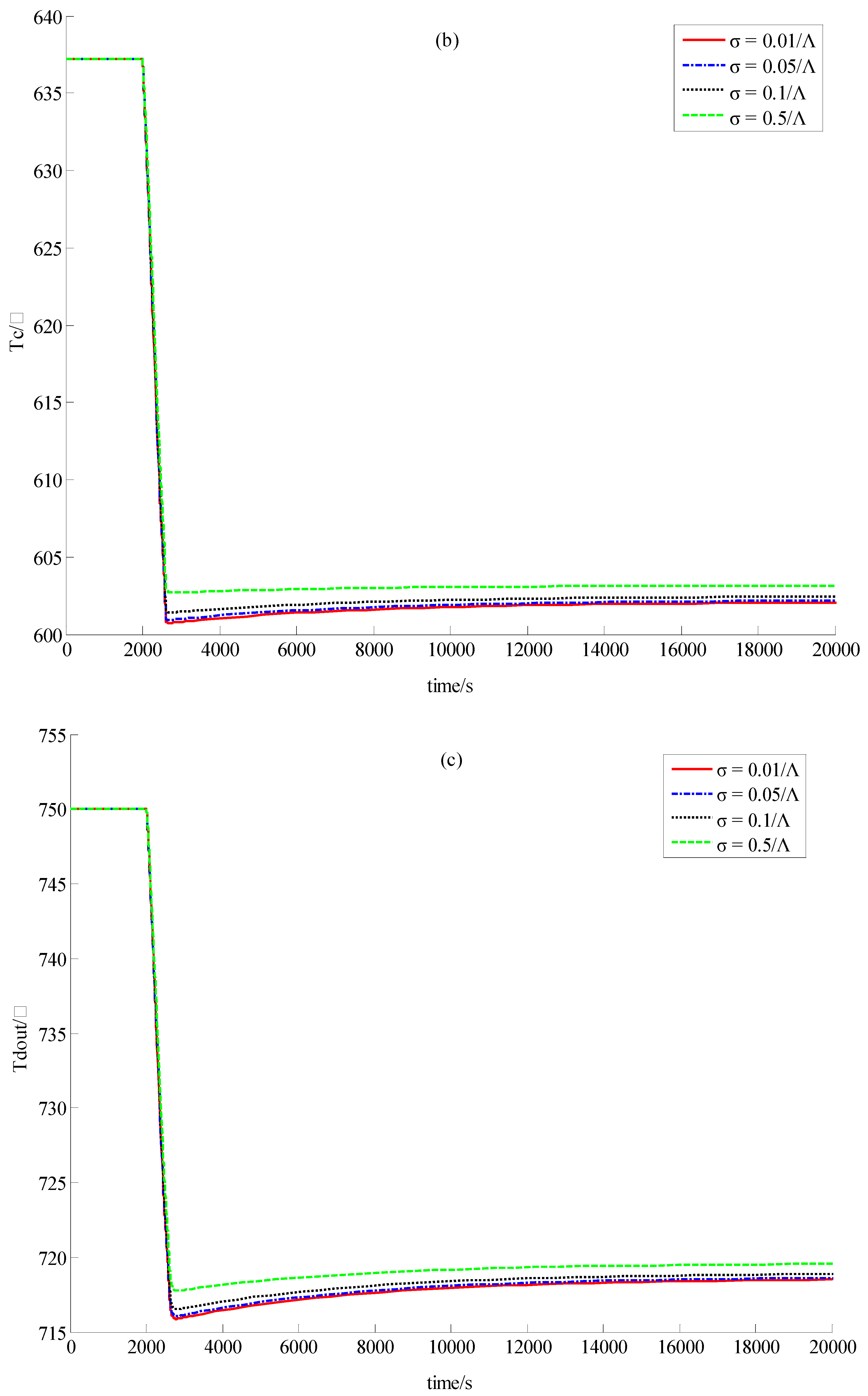
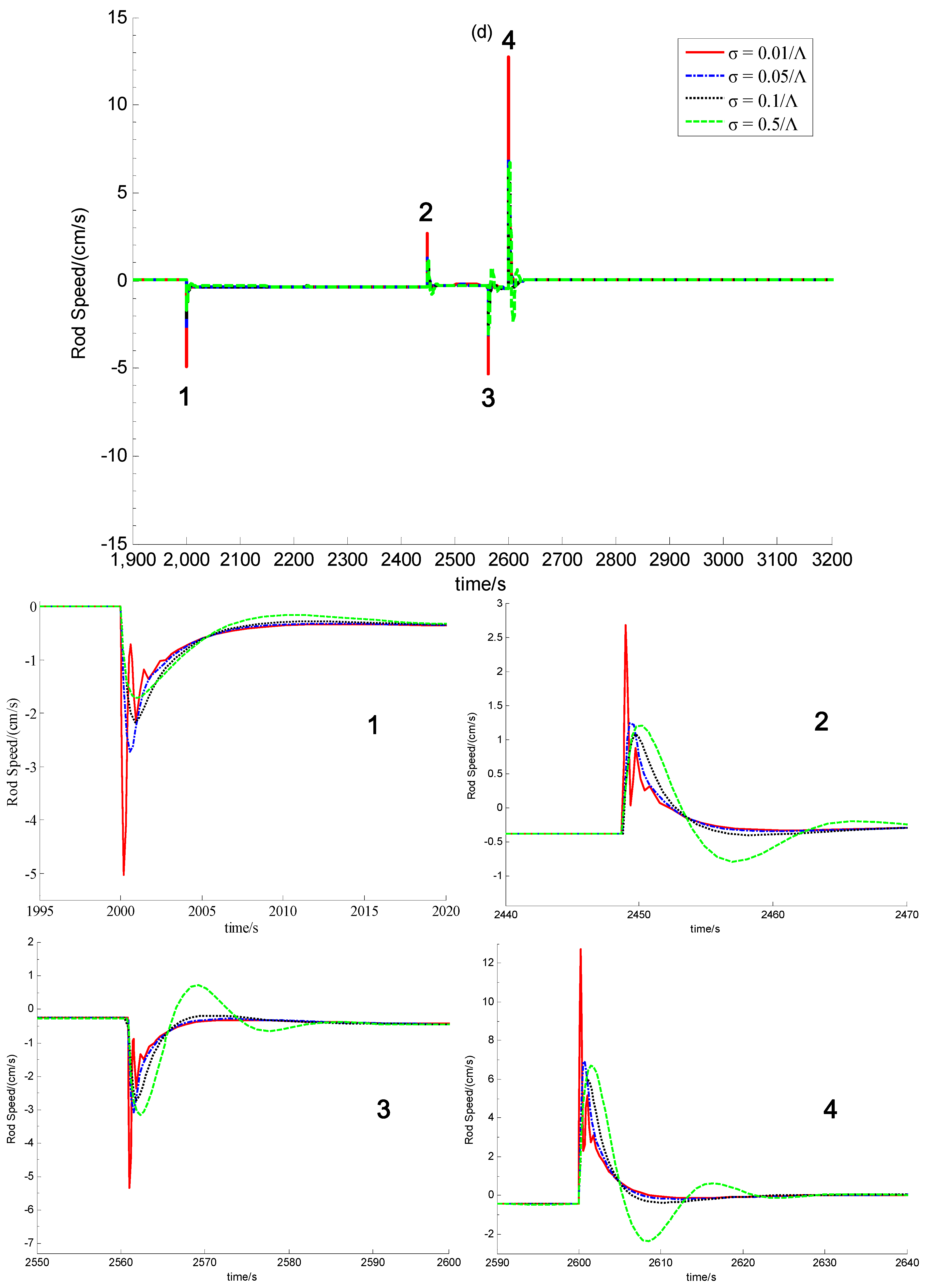
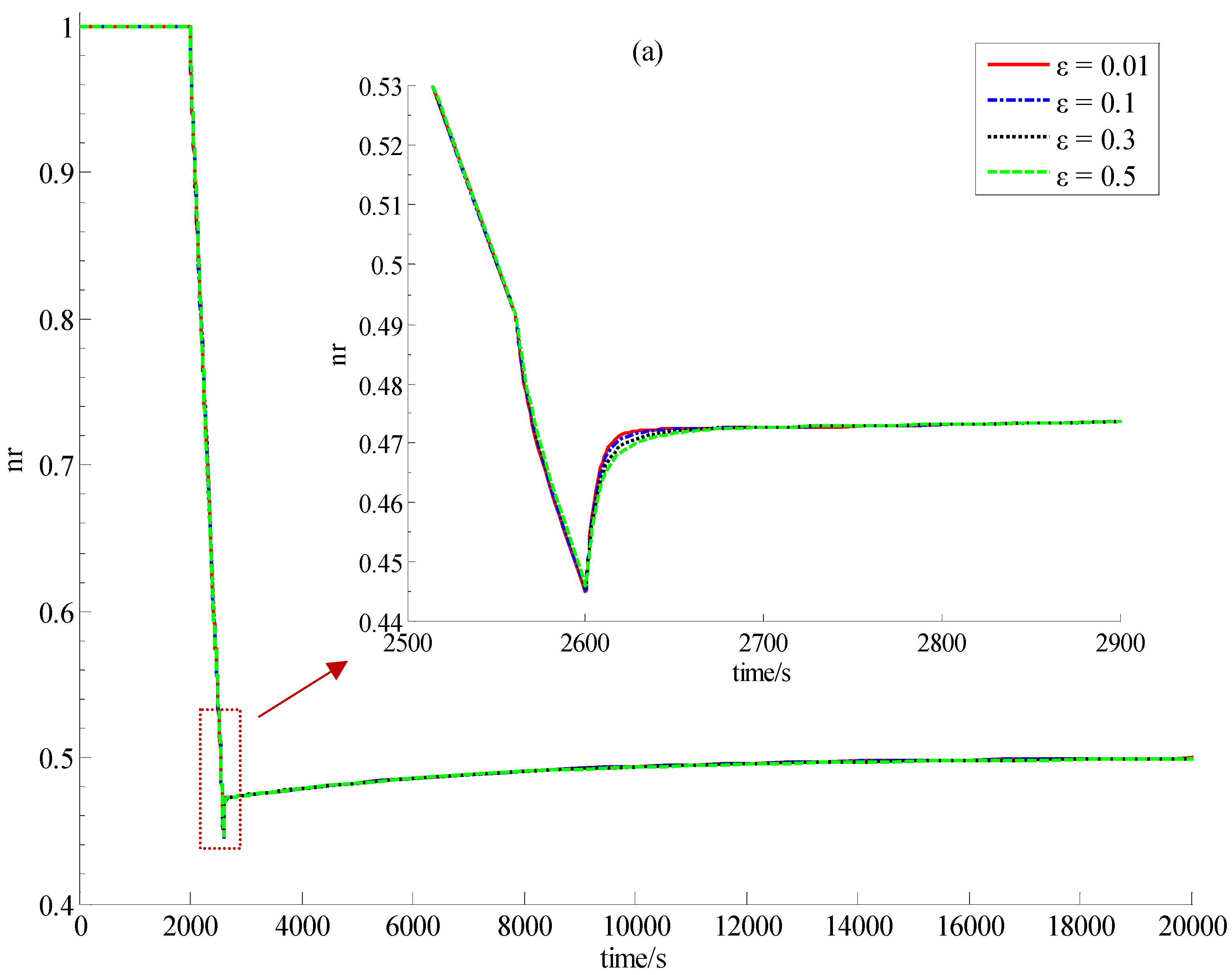
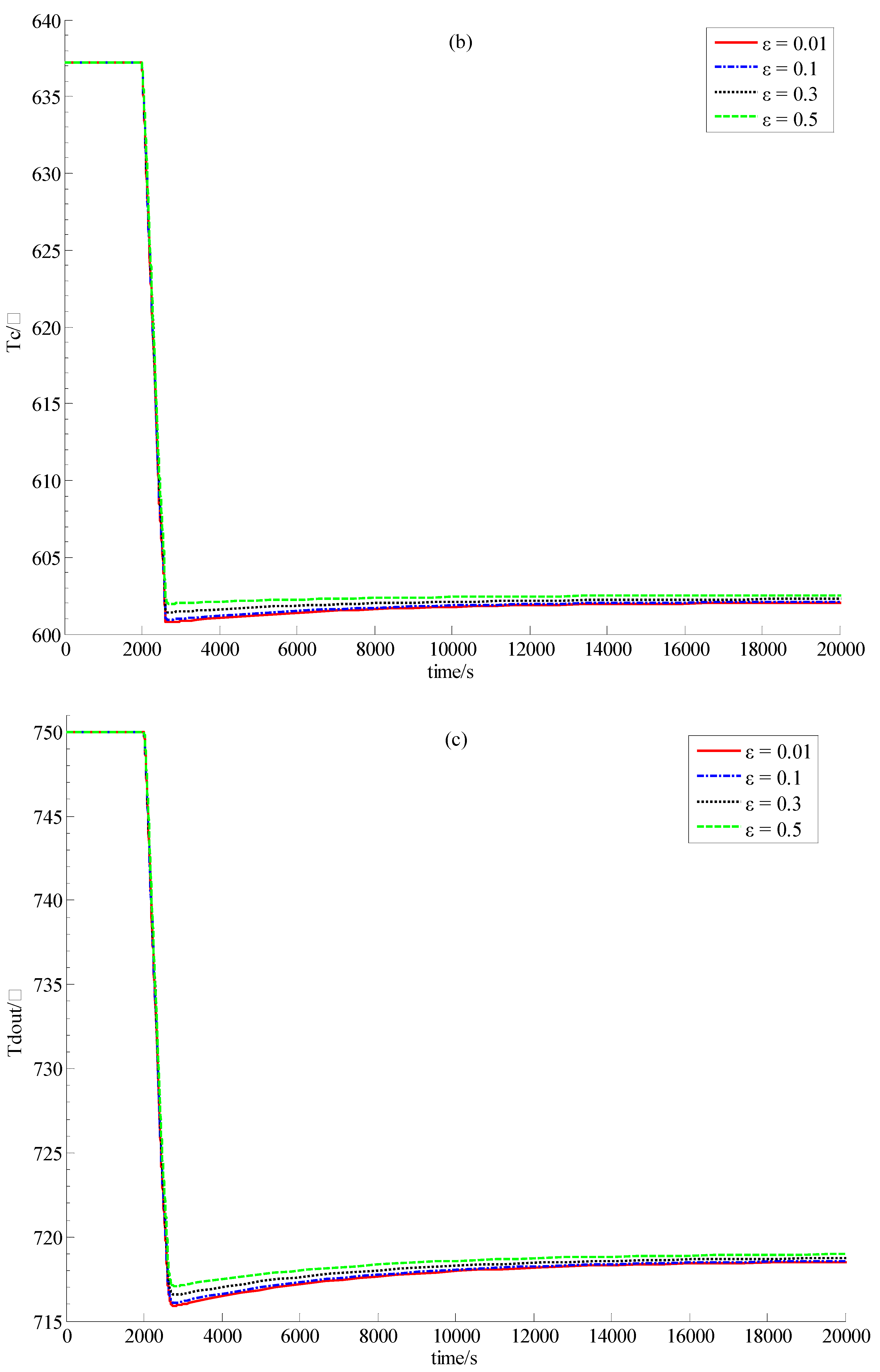
In the simulation, the following two case studies are done to show the feasibility and performance of newly-built dynamic output-feedback power-level control law Equation (79):
Case A (large power drop): power-level changes linearly from 100% to 50% in 5 minutes;
Case B (large power lift): power-level changes linearly from 50% to 100% in 5minutes.
From Equations (31,32,37,63,65,66), it is clear that since scalars C1 and C2 are so small that the influence of the value of K to the control performance is much weaker than that of σ. Therefore, in this study, we only check the influence of parameters σ and ε to the control performance.
Figure 3. Dynamic responses in Case A of (a) relative nuclear power; (b) average fuel temperature; (c) outlet helium temperature and (d) control rod speed signal with different σ and constant ε.
Energies 05 01782 g003aEnergies 05 01782 g003bEnergies 05 01782 g003c
In the numerical simulation, K is set to be 10.0, and control parameter σ and observation parameter ε are set to be different values respectively.
Case A: In this test, the power demand signal decreases down from 100% to 50% linearly with a speed of 5%/min. Corresponding to the power demand drop, both the error between the actual and the demanded power-levels and that between the actual and the referenced values of average coolant temperature become larger than before. These error signals stimulate the power-level controller to insert the control rod in order to weaken these two error signals. If scalar ε = 0.01 and σ adopts different values, then the responses of the relative nuclear power, average fuel temperature, average helium temperature and control rod speed generated by power-level controller Equation (79) during the transition period are all illustrated in Figure 3. If scalar σ = 0.01/Λ and ε is set to different values, then the corresponding dynamic responses of these concerned process variables are shown in Figure 4.
Case B: As the power demand signal rises linearly from 50% to 100% in 5 minutes, the error signals in the nuclear power and the average helium temperature cause the power regulator to generate positive speed control action and lift the control rod to reduce this error. The computed responses of reactor process variables corresponding to control action Equation (79) are illustrated in Figure 5 and Figure 6.
Figure 4. Dynamic responses in Case A of (a) relative nuclear power; (b) average fuel temperature; (c) outlet helium temperature and (d) control rod speed signal with constant σ and different ε.
Energies 05 01782 g004aEnergies 05 01782 g004bEnergies 05 01782 g004c

5.3. Discussion

From Figure 3 and Figure 4, the load decrease leads both δnr and δTd to be positive and increasing, which drives the power-level controller to give a negative control rod speed signal. Inserting the control rods leads to the decreases of both the nuclear power and fuel temperature. The closed-loop system comes into an equilibrium state if the positive reactivity caused by the decrease of the fuel temperature nearly cancels the negative reactivity caused by the rod insertion. The generation of the control rod speed signal is driven by the variations of both the nuclear power and average coolant temperature obtained from measurement. These two variation signals lead state-observer Equation (78) to give a convergent observation of the state-variations which then cause state-feedback power-level control Equation (63) to generate the speed signal of control rods. Also from Figure 3, we can see that the steady regulation error is smaller if controller parameter σ is larger. Actually, from Equation (56), it is clear that a larger σ can result in a larger L2 gain from the disturbance to the evaluation signal, which means that the closed-loop system is more robust to both the modeling uncertainty or exterior disturbances. Thus, a smaller steady control error reflects that the closed-loop system has a stronger ability to sustain the disturbances. However, from Proposition 2, to maintain the L2 disturbance attenuation property of state-feedback law Equation (56), it is necessary to set parameter ε to be a small enough positive scalar. This can be clearly seen from Figure 4 that scalar ε is larger, the L2 disturbance attenuation performance of the closed-loop is weaker.
Figure 5. Dynamic responses in Case B of (a) relative nuclear power; (b) average fuel temperature; (c) outlet helium temperature and (d) control rod speed signal with different σ and constant ε.
Energies 05 01782 g005aEnergies 05 01782 g005bEnergies 05 01782 g005c
Moreover, from Figure 5 and Figure 6, the load increase causes the decrease of δnr and δTd, which results in the generation of a positive speed signal of control rods. The withdrawal of the control rods then causes increases of both the nuclear power and the fuel temperature. Similarly with the case of load drop, the closed-system come to the steady state if the negative reactivity caused by the increase of the fuel temperature nearly cancels the positive reactivity induced by withdrawing the control rods. Moreover, it is clear from Figure 5 and Figure 6 that the control performance is also deeply influenced by the values ε and σ. The reason is the same as that given in the above paragraph.
Finally, from the theoretical analysis and numerical simulation, dynamic output-feedback control strategy Equation (79) is feasible for the power-level regulation of the MHTGRs. The L2 disturbance attenuation performance of this newly-built control law is guaranteed by choosing the values of both parameters ε and σ to be small enough. With comparison to the power-level controller presented in [29], the transition periods of both the fuel and coolant temperatures caused by the newly-built controller in this paper is much smaller than those corresponding to the controller in [29]. This is just an instance for the fact that dynamic output feedback control is stronger than static output feedback control, and this is also the key improvement of the work in this paper relative to that in [29].
Figure 6. Dynamic responses in Case B of (a) relative nuclear power; (b) average fuel temperature; (c) outlet helium temperature and (d) control rod speed signal with constant σ and different ε.
Energies 05 01782 g006aEnergies 05 01782 g006bEnergies 05 01782 g006c

6. Conclusions

Power-level control is a crucial technique for guaranteeing operation stability and efficiency of the MHTGRs. Since the dynamics of the MHTGR are nonlinear and modern state-feedback power-level control has the potential of improving closed-loop stability and control performance, it is necessary to develop a nonlinear power-level control technique for the MHTGR-based nuclear plants. Stimulated by this, a novel nonlinear dynamic output-feedback power-level controller has been given, and the two key techniques of developing this control strategy are respectively the iterative dissipation assignment (IDA) given in Section 3 and the DHGF-based observer design technique given in Section 4. This power-level control strategy can guarantee the L2 disturbance attenuation performance, and has analytic expressions with clear physical meaning. Moreover, there is a clear relationship between the controller parameters and the regulation performance. Both simulation results and theoretical analysis have shown that the performance of this newly developed power-level controller can be satisfactory high with large enough σ and ε. The results given here have shown the theoretic feasibility of this newly-developed power-level control law. For engineering implementation of this control strategy for the MHTGR such as the reactors of HTR-10 or HTR-PM, the future study lies in verifying the performance of this control strategy on the hardware-in-loop simulation platform proposed in [30].

Acknowledgement

This work is jointly supported by the Natural Science Foundation (Grant No. 61004016) and National S&T Major Project (Grant No.ZX06901) of China. The author would like to thank to the anonymous reviewers for their constructive recommendations. Further, the author would like also to thank Xiaojin Huang for valuable discussions and suggestions.

References

  1. Reutler, H.; Lohnert, G.H. The modular high-temperature reactor. Nucl. Technol. 1983, 62, 22–30. [Google Scholar]
  2. Reutler, H.; Lohnert, G.H. Advantages of going modular in HTRs. Nucl. Eng. Des. 1984, 78, 129–136. [Google Scholar] [CrossRef]
  3. Lohnert, G.H. Technical design features and essential safety-related properties of the HTR-Module. Nucl. Eng. Des. 1990, 121, 259–275. [Google Scholar] [CrossRef]
  4. Wu, Z.; Lin, D.; Zhong, D. The design features of the HTR-10. Nucl. Eng. Des. 2002, 218, 25–32. [Google Scholar] [CrossRef]
  5. Hu, S.; Liang, X.; Wei, L. Commissioning and operation experience and safety experiment on HTR-10. In Proceedings of 3rd International Topical Meeting on High Temperature Reactor Technology, Johnanneshurg, South Africa, 1–4 October 2006.
  6. Zhang, Z.; Wu, Z.; Wang, D.; Xu, Y.; Sun, Y.; Li, F.; Dong, Y. Current status and technical description of Chinese 2 × 250MWth HTR-PM demonstration plant. Nucl. Eng. Des. 2009, 239, 1212–1219. [Google Scholar] [CrossRef]
  7. Zhang, Z.; Sun, Y. Economic potential of modular reactor nuclear power plants based on the Chinese HTR-PM project. Nucl. Eng. Des. 2007, 237, 2265–2274. [Google Scholar] [CrossRef]
  8. Edwards, R.M.; Lee, K.Y.; Schultz, M.A. State-feedback assisted classical control: An incremental approach to control modernization of existing and future nuclear reactors and power plants. Nucl. Technol. 1990, 92, 167–185. [Google Scholar]
  9. Ben-Abdennour, A.; Edwards, R.M.; Lee, K.Y. LQR/LTR robust control of nuclear reactors with improved temperature performance. IEEE Trans. Nucl. Sci. 1992, 39, 2286–2294. [Google Scholar] [CrossRef]
  10. Arab-Alibeik, H.; Setayeshi, S. Improved temperature control of a PWR nuclear reactor using LQG/LTR based controller. IEEE Trans. Nucl. Sci. 2003, 50, 211–218. [Google Scholar] [CrossRef]
  11. Shtessel, Y.B. Sliding mode control of the space nuclear reactor system. IEEE Trans. Aerosp. Electron. Syst. 1998, 34, 579–589. [Google Scholar] [CrossRef]
  12. Ku, C.C.; Lee, K.Y.; Edwards, R.M. Improved nuclear reactor temperature control using diagonal recurrent neural networks. IEEE Trans. Nucl. Sci. 1992, 39, 2298–2308. [Google Scholar] [CrossRef]
  13. Na, M.G.; Hwang, I.J.; Lee, Y.J. Design of a fuzzy model predictive power controller for pressurized water reactors. IEEE Trans. Nucl. Sci. 2006, 53, 1504–1514. [Google Scholar] [CrossRef]
  14. Huang, Z.; Edwards, R.M.; Lee, K.Y. Fuzzy-adapted recursive sliding-mode controller design for power plant control. IEEE Trans. Nucl. Sci. 2004, 51, 1504–1514. [Google Scholar] [CrossRef]
  15. Van der Schaft, A.J. L2-Gain and Passivity Techniques in Nonlinear Control; Springer: Berlin, Germany, 1999. [Google Scholar]
  16. Maschke, B.M.; Ortega, R.; van der Schaft, A.J. Energy-based Lyapunov functions for forced Hamiltonian systems with dissipation. IEEE Trans. Autom. Control 2000, 45, 1498–1502. [Google Scholar] [CrossRef]
  17. Ortega, R.; van der Schaft, A.J.; Maschke, B.M.; Escobar, G. Interconnections and damping assignment passivity-based control of port-controlled Hamiltonian systems. Automatica 2002, 38, 585–596. [Google Scholar] [CrossRef]
  18. Ortega, R.; van der Schaft, A.J.; Castaños, F.; Astolfi, A. Control by interconnection and standard passivity-based control of port-Hamiltonian systems. IEEE Trans. Autom. Control 2008, 53, 2527–2542. [Google Scholar] [CrossRef]
  19. Ortega, R.; Spong, M.W.; Gómez-Estern, F.; Blankenstein, G. Stabilization of a class of underactuated mechanical systems via interconnection and damping assignment. IEEE Trans. Autom. Control 2002, 47, 1218–1233. [Google Scholar] [CrossRef]
  20. Fujimoto, K.; Sugie, T. Stabilization of Hamiltonian systems with nonholonomic constraints based on time-varying generalized canonical transformations. Syst. Control Lett. 2001, 44, 309–319. [Google Scholar] [CrossRef]
  21. Liu, Q.J.; Sun, Y.Z.; Shen, T.L.; Song, Y.H. Adaptive nonlinear coordinated excitation and STATCOM controller based on Hamiltonian structure for multimachine power-system stability enhancement. IET Proc. Control Theory Appl. 2003, 50, 285–294. [Google Scholar] [CrossRef]
  22. Wang, Y.; Cheng, D.; Li, C.; Ge, Y. Dissipative Hamiltonian realization and energy-based L2-disturbance attenuation control of multi-machine power systems. IEEE Trans. Autom. Control 2003, 48, 1428–1433. [Google Scholar] [CrossRef]
  23. Galaz, M.; Ortega, R.; Bazanella, A.S.; Stankovic, A.M. An energy-shaping approach to the design of excitation control of synchronous generators. Automatica 2003, 39, 111–119. [Google Scholar] [CrossRef]
  24. Dong, Z.; Feng, J.; Huang, X.; Zhang, L. Dissipation-based high gain filter for monitoring nuclear reactors. IEEE Trans. Nucl. Sci. 2010, 57, 328–339. [Google Scholar] [CrossRef]
  25. Dong, Z.; Huang, X.; Zhang, L. Output feedback power-level control of nuclear reactors based on a dissipative high gain filter. Nucl. Eng. Des. 2011, 241, 4783–4793. [Google Scholar] [CrossRef]
  26. Li, H.; Huang, X.; Zhang, L. A simplified mathematical dynamic model of the HTR-10 high temperature gas-cooled reactor with control system design purpose. Ann. Nucl. Energy 2008, 35, 1642–1651. [Google Scholar] [CrossRef]
  27. Dong, Z.; Huang, X.; Zhang, L. A nodal dynamic model for control system design and simulation of an MHTGR core. Nucl. Eng. Des. 2010, 240, 1251–1261. [Google Scholar] [CrossRef]
  28. Li, H.; Huang, X.; Zhang, L. A lumped parameter dynamic model of the helical coiled once-through steam generator with movable boundaries. Nucl. Eng. Des. 2008, 238, 1657–1663. [Google Scholar] [CrossRef]
  29. Dong, Z. Output feedback dissipation control for the power-level of modular high-temperature gas-cooled reactors. Energies 2011, 4, 1858–1879. [Google Scholar] [CrossRef]
  30. Dong, Z.; Huang, X. Real-time simulation platform for the design and verification of the operation strategy of the HTR-PM. In Proceedings of the 19th International Conference on Nuclear Engineering, Chiba, Japan, 16–19 May 2011.

