1. Introduction
Are there trade-offs between energy use and greenhouse gas emissions for different types of passenger cars? In order to answer this question, we have performed an energy chain analysis that addresses three questions:
What is the direct energy consumption for the car’s propulsion? What are the corresponding greenhouse gas emissions measured in CO2-equivalents?
What are the energy consumption and greenhouse gas emissions associated with the production of propulsion energy?
What are the embodied energy and greenhouse gas emissions for the construction, maintenance, and operation of the passenger car’s infrastructure and of the car itself?
In 2010, transport in the EU accounted for a third of total energy consumption and more than a fifth of all greenhouse gas emissions [
1]. For most transport modes, the growth in volumes is greater than growth in the energy efficiency, thereby leading to an increasing impact of transport on greenhouse gas emissions. The total energy consumption worldwide for light-duty vehicles in 2000 was 34.2 EJ, which was 44.5% of total energy consumption from all transport modes that year [
2]. Transport volumes are also growing fast; the annual growth is 1.9% for passenger transport and 2.7% for freight transport. For most transport modes, the growth in volumes is greater than growth in energy efficiency, thereby leading to an increasing impact of transport on greenhouse gas emissions and energy consumption.
With this background, it is generally agreed internationally that we currently have an unsustainable transport system [
3,
4,
5]. Furthermore, it is generally agreed that, without significant changes in policy and practice, the unsustainable trend will continue. A necessary condition for successful change of policy and practice is knowledge about various transport means and their total environmental impact.
This article is based on a larger study done by the Western Norwegian Research Institute from 2008 to 2010 for Research Council Norway [
6]. The project’s objective was to establish a consistent energy and emissions database for passenger and freight transport. The database includes vehicles for road, sea and air transport and also includes both conventional and alternative energy sources and fuels. Vehicle passenger transport is distributed on main travel categories. Since passenger car transport represents a considerable share of total transport environmental impact, it is very difficult to achieve a reduction in energy consumption and a mitigation of greenhouse gas emissions without a substantial contribution from passenger car transport.
The object of this article is to discuss whether there are trade-offs between energy consumption and greenhouse gas emissions for certain passenger car fuels and drivetrains. If there is such a trade-off for certain fuels then the mitigation of energy consumption and greenhouse gas emissions by using them will be limited. The following drivetrains and fuels are studied in this article: (a) internal combustion engines with conventional fuels like gasoline and diesel in addition to alternative biofuels; (b) battery-powered vehicles using electricity as fuel; (c) fuel cell vehicles using hydrogen from natural gas or electrolysis of water as fuel; and d) hybrids using electricity from batteries together with gasoline and diesel in a combustion engine.
2. Earlier Studies
One of the first studies in Norway using a life cycle perspective in analysis of energy consumption in transport systems was carried out by Høyer and Heiberg [
7]. They included three life cycles in their analysis, Well-to-Wheel, production and maintenance of transport means and construction, maintenance and operation of transport systems’ infrastructure. The energy consumption was analyzed for different types of travel (short and long trips) and for different types of energy sources (compressed natural gas (CNG), methanol, hydrogen). Their study showed that when all life cycles were included, train, tram and subway had the lowest energy consumption while airplane and express passenger boat had the highest. Their study also showed that alternative fuels, with the exception of electricity from Norwegian hydropower, did not substantially reduce the energy consumption for passenger car transport.
A study from MIT [
8] analyzed expected energy consumption and emissions from passenger car transport with different engine technologies in 2020. The study covered pure combustion engines (gasoline, diesel), hybrids combining combustion engines with electrical engines and fuel cells and battery powered electric cars. The analysis included two life cycle stages for passenger car transport; these were vehicle propulsion including fuel production and vehicle manufacturing. Hybrids with a diesel combustion engine combined with an electrical engine had the lowest energy consumption, followed by a hybrid combining a CNG combustion engine with an electrical engine and a similar hybrid using a gasoline combustion engine.
Horvath and Chester [
9] analyzed passenger car transport together with other passenger transport systems such as buses, trains and air travel. They included in their analysis energy consumption and emissions arising from construction, operation and maintenance of the transport systems’ infrastructure in addition to the stages analyzed by MIT. They found that, when all life cycles for passenger car transport were taken into consideration, energy consumption and emissions of greenhouse gases increased by a factor of 1.4 compared to figures for vehicle propulsion alone.
Concawe/Eucar [
10,
11] is a collaboration project between the EU’s Joint Research Centre, the European Council for Automotive Research and Development (Eucar) and the oil industry’s organization for research on environmental, safety and health issues (Concawe). They published a Tank-to-Wheels and a Well-to-Tank report in March, 2007. The term Tank-to-Wheels corresponds to the term net direct energy consumption or propulsion energy. The term Well-to-Tank corresponds to the term gross direct energy addition or the fuels’ life cycle. This is the energy consumption for producing and distributing the fuel required for propulsion of the vehicle. Their Tank-to-Wheels estimates are based on data simulations of a “standard European driving cycle” for a 5-seater family sedan in the VW Golf-class.
The estimates from Concawe/Eucar cover the conventional fuels diesel and gasoline as well as biodiesel from rape seed, sunflower, soya beans and palm oil and ethanol from sugar beet, sugar cane, wheat and wood. These estimates are for combustion engines. In addition, estimates are given for hydrogen from natural gas, coal and from electrolysis of water. Electricity for electrolysis of water comes from wind power, natural gas and wood. Hydrogen is used to power fuel cells which generate electricity for an electrical engine.
DeLucchi [
12] gives estimates for Tank-to-Wheels and Well-to-Tank energy consumption and emissions of greenhouse gases for combustion engines, fuel cell vehicles and battery powered vehicles (electric cars). Some fuels, like gasoline, ethanol and hydrogen are used both in combustion engines and in fuel cell vehicles. Ethanol comes from lignin in wood or grass and starch from corn. Hydrogen comes from coal, natural gas, wood, and electrolysis of water. Hydrogen from coal, wood and electrolysis of water is used only in fuel cell vehicles while hydrogen from natural gas is used both in combustion engines and in fuel cell vehicles. Electricity for battery powered vehicles comes from fossil fuels (petroleum, coal, natural gas) as well as from wood, solar power and nuclear power. DeLucchi does not give estimates for diesel or biodiesel for passenger cars. His driving cycle is based on combined city and highway driving.
DeLucchi finds that passenger car fuel from natural gas scores lowest on energy consumption when the whole gross direct energy chain (Well-to-Wheel) is taken into consideration. Conventional gasoline is ranked before hydrogen which again is ranked before ethanol. The ethanol fuels have an energy consumption which is about 1.7 times higher than conventional gasoline for the whole gross direct energy chain.
In the net direct energy chain (Tank-to-Wheel), hydrogen ranks the best followed by ethanol and natural gas while conventional gasoline has the highest rank among these fuels. In the gross direct energy chain addition (Well-to-Tank), natural gas has the lowest rank followed by conventional gasoline and hydrogen while ethanol has the highest rank. In this energy chain, the energy consumption for ethanol is about 4.2 times higher than for conventional gasoline while the corresponding figure for hydrogen relative to conventional gasoline is about 3.9.
Høyer and Holden [
13] analyzed sixteen different energy chains with alternative and conventional fuels. Their estimates are valid for 2010. They provided estimates for diesel and gasoline from raw oil, liquefied petroleum gas (LPG), CNG, compressed gaseous hydrogen and liquefied hydrogen from natural gas, electricity from hydropower, compressed gaseous hydrogen from electrolysis of water and methanol and ethanol from biomass. The fuels were used in conventional drivetrains, hybrids (for gasoline, diesel and natural gas in combination with an electrical engine), fuel cell vehicles (using hydrogen from natural gas, methanol and ethanol with on-board reformers) and battery powered engines.
Høyer and Holden found a potential for a reduction of energy consumption for the conventional fuels, especially for diesel. They also found that none of the alternative fuels “...seem to offer a substantial reduction in total energy use compared to the best conventional options”. Electrical cars performed best, with least energy consumption, but the authors questioned whether electric cars will be a realistic option in 2010, given their low driving ranges. Fuels with biomass had the highest energy consumption, even when they are used in fuel cells.
The authors claimed that reductions in emissions of greenhouse gases from hydrogen are substantial compared to conventional fuels while reductions from biomass fuels are “considerable”. Cars running on electricity from hydropower have virtually no emissions. It should be noted that practically all Norwegian electricity is produced from hydropower.
According to Høyer and Holden, energy chains from biomass that perform the best regarding emissions of greenhouse gases, perform the worst regarding energy consumption. They estimated a measure of total environmental impact for each energy chain by ranking the chains separately for energy consumption, emissions of greenhouse gases and emissions of NOx. The ranks were added together by assuming equal weight for each impact. The authors found that the conventional fuels perform worst while natural gas based energy chains perform best. The energy chains from biomass were scattered all over the middle of the distribution with ethanol in a conventional drivetrain performing the worst and methanol in a fuel cell performing the best.
Høyer and Holden pointed out that in order to obtain sustainable transport, a fuel must score favourably on all forms of environmental impact. To check this, they computed each fuel’s difference in rank from highest to lowest for the three types of environmental impact. If fuels score consistently well or less well, this difference should, on average, approach zero. The average difference is 7.4 and the maximum difference in rank for each impact is 15. So the average difference in rank is half of the maximum attainable for every impact which suggests that fuels are favourable on some but unfavourable on others. There is no single “best” fuel. Therefore, no alternative fuel meets the sustainable mobility requirements. This implies that sustainable mobility cannot be achieved by simply switching from one fuel to another; sustainable mobility is not feasible without a reduction in overall mobility level.
This article is in many ways a continuation of the work done by Høyer and Holden. However, we include energy consumption and emissions from constructing, maintaining and operating the car’s infrastructure as well as from manufacturing the car itself in addition to the energy chains studied by Høyer and Holden. We also include biomass fuel from several feedstocks. Conventional fuels and biomass fuels are used in conventional drivetrains. On the other hand fuel cell drivetrains are only powered with hydrogen. We have no estimates for natural gas used in an internal combustion engine or in a hybrid.
Infrastructure for cars is analyzed by [
9,
14,
15,
16]. They discuss the question of allocating infrastructure use between different forms of passenger transport and between freight and passenger transport using the same infrastructure. We will present a different approach for this allocation.
We start by presenting the methodology and methodological challenges involved in analysing energy chains for passenger car transport. This is followed by a presentation of different fuels used in passenger cars. Finally, we present the results from the analysis and discuss whether the results are compatible with sustainable mobility.
3. Methodology
The methodology as used here refers both to the assumptions underlying the research process and to the actual methods applied in our article [
17]. Triangulation can be applied to data, to methods or to whole theories. We have applied data and methodological triangulation in our analysis. Methodological triangulation means employing different methods in arriving at estimates for the same process. These estimates could be made by applying different methods, such as economic input-output analysis, engineering process analysis and hybrid variations of the two. This approach is called between-method triangulation [
18] because different methods are used for the same case or estimate. Another approach is the within-method triangulation, which uses the same method for different cases.
Data triangulation implies collection of information on the same phenomenon from multiple sources with the purpose of corroborating the same fact [
18]. This involves using different estimates for the same process where the aim is to crosscheck them against each other.
By comparing estimates of the same process made with different methods, we are forced to consider and re-evaluate their assumptions. With a critical reconstruction of the assumptions, we have a better chance of finding estimates that are comparable in a consistent and cohesive manner. Used in this way, triangulation could improve both the reliability and the validity of the estimates.
Our triangulation method has started with a critical analysis of various literature sources [
8,
9,
10,
11,
12,
13,
19]. Some estimates are based on a single source, whereas other estimates are a combination of sources. As a basic unit for comparison we use energy expressed in megajoules (MJ). We choose to concentrate on energy consumption because it is strongly associated with environmental problems created by the production, transport, transmission and application of energy. There is a relationship between energy consumption and greenhouse gas emissions, but energy consumption also involves several dimensions not related to greenhouse gas emissions, such as land and resource use. There is a close link between energy consumption and associated environmental problems. High energy consumption is therefore an environmental challenge in itself [
7,
20].
In addition, we produce estimates for greenhouse gas emissions. These include include carbon dioxide (CO
2), methane (CH
4), nitrous oxide (N
2O), hydro- and perfluorocarbons (HFCs, PFCs) and sulphur hexafluoride (SF
6). The decay period for all gases is assumed to be 100 years [
21].
This implies that we have omitted regional and local emissions as well as the impact on land use from our analysis. We have chosen to focus the study on two key indicators, energy consumption and the related emissions of greenhouse gases.
In order to analyze whether there is a trade off between energy consumption and greenhouse gas emissions, we will perform some statistical tests. By performing these statistical tests we can answer this question in a more systematic way. We have chosen a statistical test based on a regression analysis and a non-parametric sign test. Both tests use energy consumption and greenhouse gas emissions ranks as input. One of the test implies an assumption of normal distribution (regression analysis) while the other (sign test) does not. Therefore, comparison of test results should indicate whether this assumption is reasonable.
We analyze passenger car transport in three different energy chains. Net direct energy consumption and associated emissions includes the energy used to operate the means of transport, that is, the vehicles’ propulsion energy. Methodological concerns in this phase are linked to vehicle technology and the physical properties of the fuel. The assumptions of energy and carbon content of different fuels, for example, will have an influence on the expected direct energy use and greenhouse gas emissions.
The term
gross direct energy consumption includes the net direct energy consumption plus the energy it takes to produce this energy. Together they constitute the life cycle of the fuel. This includes all energy losses and emissions in the production, conversion and distribution of energy. We use the term
primary energy to indicate that energy required for conversion of energy sources into end-use energy is taken into consideration. This type of study was initially referred to as
fuel chain or
energy chain analysis of transportation energy consumption [
22]. Recently it has become more common to describe it as Well-to-Wheel (WtW) analysis—a sort of cradle-to-grave analysis of transportation energy consumption. For passenger cars, this is equal to the gross direct energy chain, which consists of
Extraction/production of the energy source;
Transportation of the energy source;
Production of the energy carrier (fuel, electricity);
Distribution of the energy carrier;
The net direct energy consumption, this is the energy applied for passenger car propulsion.
The net direct energy chain is often referred to as the Tank-to-Wheel energy chain whereas the additional energy consumption in the gross direct energy chain is referred to as the Well-to-Tank energy chain. The whole gross direct energy chain is referred to as Well-to-Wheel energy chain. For passenger cars, these concepts are quite intuitive; this, however, is not the case for other transport systems. Where does the well end, and the tank start, for an electrified railway transport system?
The third term to consider is the indirect energy consumption that covers the life cycles of the vehicle and the infrastructure. For passenger cars, this includes the energy required to build and operate the roads as well as energy required to manufacture and maintain the car itself. We refer to this as embedded energy in materials and equipment necessary for passenger car transport.
Besides conventional fuels such as gasoline and diesel, we have included the following alternative fuels in this paper: biofuels (ethanol, biodiesel), hydrogen and electricity. All electricity is assumed to come from Norwegian hydropower. Hydrogen is produced from reforming of natural gas or from electrolysis of water. Ethanol comes from corn, sugar cane, sugar beet or wheat, while biodiesel is produced from rapeseed or sunflowers. The following drivetrains are studied in this article: (a) internal combustion engines with conventional fuels like gasoline and diesel in addition to alternative biofuels; (b) battery-powered vehicles using electricity as fuel and; (c) fuel cell vehicles using hydrogen from natural gas or electrolysis of water as fuel. In addition, hybrids using electricity from batteries together with gasoline and diesel in a combustion engine are included in the analysis. In our selection of fuels and powertrains, we have basically applied the same principles as Høyer and Holden [
13]. The feedstock must be available in large quantities, the technologies must have potential to be commercially viable, and the alternative cars must have an expected potential for mitigation of environmental impacts.
Infrastructure analysis raises three major methodological concerns: (1) Where should we set system boundaries? (2) Are all relevant emissions and energy consumption included? (3) How should we allocate resources between means of transport using the same infrastructure? Especially important in this context is the definition of the system boundaries: What is to be included in the analysis, and what is to be left out? Should gas stations and repair shops be included in the car’s infrastructure? If so, the transport system would be more comparable with rail infrastructure, which usually includes railway stations and repair yards for trains. We have kept filling stations, repair shops and similar facilities out of the passenger car infrastructure because they are not directly required for its operation.
A special methodological challenge is linked to allocation of infrastructure between different transport means using it concurrently. A road is used by cars, vans, trucks, and buses. How should we allocate energy use end emissions related to construction, maintenance and operation of the infrastructure among them? In this paper, we will use passenger car equivalents for this allocation. The construction and application of these equivalents will be described in a later section.
For road construction, we have based our analysis on Norwegian conditions. The impact from infrastructure construction, maintenance and operation will differ somewhat according to proportion of tunnels and bridges. Also, the allocation of infrastructure on different transport modes that share it may be different in different countries, depending on characteristics such as road curvature, gradients and maximum freight load allowed.
We have based our estimate for the electric car on Norwegian conditions using hydropower as electric source. Electric cars in other countries than Norway would not have the same performance since electricity in Norway is produced almost exclusively from hydropower. Except for road construction and the assumption of hydropower for electric cars, the rest of the key assumptions are mainly valid for general European conditions.
In this paper, we assume that the energy consumption (and greenhouse gas emissions) related to infrastructure is identical for all types of cars. This is in line with Notter
et al. [
23].
The manufacturing of cars also requires energy. In order to arrive at credible estimates, it is essential to include both consumed process energy and embedded energy in materials. The results will also depend on what kind of recycling level is applied for different type of materials.
We have not included energy requirements and emissions related to disposing of passenger cars and their infrastructure. We have chosen this approach because the impact from disposing is minor relative to energy consumption and greenhouse gas emissions in other energy chains [
23,
24]. Also, this paper is part of a larger study comparing several transport systems. It was difficult to find estimates for vehicle and infrastructure disposal for most other transport systems. Therefore, since disposal plays a limited role in the overall environmental impact, we chose not to include it.
We have chosen 2010 as a time reference for our estimates. However, some of the fuel alternatives that we analyze are not yet fully commercially available; the same is true for some of the drivetrains. We have still chosen to include these alternatives because we expect these fuels and drivetrains to play an important role in future passenger car transport.
The following sections will present the assumptions we make for the various energy chains regarding energy consumption and greenhouse gas emissions. We are concerned about presenting assumptions as transparent as possible so that they can be critically reviewed by others.
4. Gross Direct Energy Chain (Well-to-Tank)
The estimates for these energy chains are mostly obtained from Concawe/Eucar [
10,
11] The estimate for Norwegian hydro power is from [
22]. Some estimates are obtained from the German LCA-database ProBas [
19]. We consider it favourable to use many estimates from the same source as these are more likely to have the same consistent demarcation of the energy chains.
A loss multiplier tells us how much
more energy that is required to produce one unit of energy from the fuels feedstock’s. Loss of energy content in feedstock during transformation to usable energy is included in the calculation of the loss multiplier. Loss multipliers have one attractive property. They are unit free meaning that any energy production can be measured by a multiplier regardless of what unit the energy production is measured in. Equation 1 shows the formula for calculating loss multipliers:
The inverse of the loss multiplier is the efficiency of the fuel, the proportion of the energy content in the feedstock available for final consumption.
Equation 2 shows how energy consumption in the WTT energy chain is calculated by using propulsion energy (TTW) and the loss multiplier:
For all fuels, energy consumption required for road depot and filling stations is included in the estimates.
Table 1 shows the energy consumption pr MJ of energy fuel delivered.
Table 1.
Energy consumption pr MJ of fuel energy delivered.
Table 1.
Energy consumption pr MJ of fuel energy delivered.
| Electricity | MJ Expended/MJ Content in Fuel |
|---|
| Road depot | 0.00084 |
| Filling stations | 0.00340 |
Equation 3 shows the formula for calculating additional emissions of CO
2-equivalents pr vehicle-km in the gross direct energy chain (Well-to-Tank chain). These are emissions related to producing fuel for vehicle propulsion (Tank-to-Wheel chain). Since the energy required for propulsion dimensions emissions in the production step, the propulsion energy pr vehicle km should be multiplied with emissions of CO
2 equivalents in gram pr MJ from this step:
4.1. Ethanol Fuels
For all ethanol fuels, cellulose as left over material from production of ethanol is used as animal fodder. The energy required for this co-production is allocated on the fodder and not on the ethanol. Also, production of 1 MJ of steam used as process heat requires 1.111 MJ of natural gas and 0.02 MJ of electricity.
Table 2 shows the non-cumulative primary energy use for production of 1 MJ of energy from ethanol from different feedstocks.
Table 3 shows the CO
2-equivalents pr MJ for production of ethanol from different feedstocks in the Well-to-Tank energy chain
The estimates are obtained from Concawe/Eucar. The energy content of the feedstock is included in the calculation; therefore the sum of non-cumulative energy consumption relative to the output is the loss multiplier. For sugar beet, i.e., we need to use almost 1.4 times the energy content of the final product in order to transform feedstock to usable energy. The efficiency of ethanol from sugar beet is the inverse of this multiplier which is 0.57.
Table 2.
Loss multipliers for biodiesel from different feedstocks for ethanol from different feedstocks.
Table 2.
Loss multipliers for biodiesel from different feedstocks for ethanol from different feedstocks.
| MJ Expended/MJ Content in Fuel | Ethanol Feedstock |
| Activity | Sugar beet | Wheat | Corn |
| Cultivation | 1.391 | 1.283 | 1.269 |
| Road transport 30 km | 0.011 | 0.006 | 0.004 |
| Ethanol at plant | 0.332 | 0.375 | 0.145 |
| Ethanol road transport (150 km to depot, 150 km from depot to tank facility) | 0.016 | 0.016 | 0.016 |
| Tank facility | 0.010 | 0.010 | 0.010 |
| Sum | 1.759 | 1.689 | 1.443 |
Table 3.
Emissions of gram CO2-equivalents pr MJ for production of ethanol from different feedstocks in the Well-to-Tank energy chain.
Table 3.
Emissions of gram CO2-equivalents pr MJ for production of ethanol from different feedstocks in the Well-to-Tank energy chain.
| Gram CO2-Equivalents pr MJ in Final Fuel | Definitions | Sugar Beet | Wheat | Corn |
|---|
| Cultivation | A | 11.5 | 23.4 | 20.2 |
| Road transport 30 km | B | 0.8 | 0.4 | 0.3 |
| Ethanol at plant | C | 18.9 | 13.6 | 15.0 |
| Ethanol road transport (150 km to depot, 150 km from depot to tank facility) | D | 1.1 | 1.1 | 1.1 |
| Tank facility | E | 0.4 | 0.4 | 0.4 |
| Total WTT emissions gram CO2-equivalents/MJ | F = A + B + C + D + E | 32.8 | 38.9 | 37.0 |
| Propulsion MJ/vehicle-km TTW | G | 1.879 | 1.879 | 1.879 |
| Emissions CO2-eq/vehicle-km WTT | H = F × G | 61.6 | 73.2 | 69.5 |
4.2. Biodiesel
For all biodiesel fuels, glycerol is a by-product from transesterification of biodiesel. Energy consumed for production of glycerol is subtracted from energy required for biodiesel production.
Table 4 shows primary energy use for production of 1 MJ of energy from biodiesel from different feedstock. The estimates are obtained from Concawe/Eucar.
Table 5 shows emissions of CO
2-equivalents from production of biodiesel from different feedstocks.
The estimate for biodiesel from animal fat or tallow (TME, tallow-methyl-ester) is obtained by combining estimates from Concawe/Eucar with an estimate for the production of TME in Germany 2000. The latter estimate is obtained from [
17]. The German database also has an estimate for RME, but this is older than the estimate from Concawe. We have assumed the same relative difference between biodiesel from RME and TME in 2010 as in 2000. This approach gives us an estimate for TME based on the ProBas estimate from 2000 but adjusted to 2010 by using the RME estimate from Concawe/Eucar.
Table 4.
Loss multipliers for biodiesel from different feedstocks.
Table 4.
Loss multipliers for biodiesel from different feedstocks.
| MJ Expended/MJ Content in Fuel | Biodiesel Feedstock |
| Activity | Rape Seed | Sunflower Seed | Soya Beans |
| Cultivation | 1.172 | 1.128 | 1.104 |
| Drying | 0.009 | 0.009 | 0.038 |
| Road transport, 50 km | 0.002 | 0.002 | 0.113 |
| Fabrication plant, rape seed oil | 0.049 | 0.049 | 0.098 |
| Transesterification | 0.213 | 0.213 | 0.213 |
| Road transport 150 km to depot, 150 km from depot to tank facility | 0.012 | 0.012 | 0.012 |
| Tank facility | 0.010 | 0.010 | 0.010 |
| Sum | 1.467 | 1.423 | 1.588 |
Table 5.
Emissions of gram CO2-equivalents pr MJ for production of biodiesel from different feedstocks in the Well-to-Tank energy chain.
Table 5.
Emissions of gram CO2-equivalents pr MJ for production of biodiesel from different feedstocks in the Well-to-Tank energy chain.
| Gram CO2 Equivalents pr MJ in Final Fuel | Definitions | Biodiesel-Rapeseed (RME) | Biodiesel-Sunflower (SME) | Biodiesel-Soya Beans |
|---|
| Cultivation | A | 28.5 | 17.2 | 18.6 |
| Drying | B | 0.4 | 0.4 | 2.9 |
| Road transport, 50 km | C | 0.2 | 0.2 | 8.9 |
| Fabrication plant, rape seed oil | D | 2.7 | 2.7 | 5.5 |
| Transesterification | E | 12.8 | 12.8 | 12.8 |
| Road transport 150 km to depot, 150 km from depot to tank facility | F | 0.8 | 0.8 | 0.8 |
| Tank facility | G | 0.4 | 0.4 | 0.4 |
| Total WTT emissions gram CO2-equivalents/MJ | H = A + B + C + D + E + F + G | 45.9 | 34.6 | 49.9 |
| Propulsion MJ/vehicle-km TTW | I | 1.657 | 1.657 | 1.657 |
| Emissions CO2-eq/vehicle-km WTT | J = H × I | 76.0 | 57.3 | 82.6 |
4.3. Ethanol from Sugar Cane
The estimate for ethanol from sugar cane is based on Macedo and Seabra [
25]. Production of ethanol from sugar cane starts with extracting the sugar from the sugar cane plant. The sugar in the plant is extracted by pressing the plant, releasing the starch and break down the starch to sugar. The resulting juice is transformed to ethanol by fermentation.
Macedo and Seabra provide three estimates for sugar cane ethanol, two of them are for 2020 and one for 2010. The estimates differ in the use of residual plant material from ethanol production. We have used the 2010 estimate which does not include any use of surplus plant material. This estimate reflects current sugar cane ethanol production in Brazil.
Emissions of CO2-equivalents in the production phases come from cultivation of the plant, transport of feedstock to production plant and from building and maintaining the production facilities. Additionally, burning of sugar cane before harvesting generate emissions. Burning the plant alleviates the harvesting of it.
The production model which the estimate is based on yields 87.1 tonne sugar cane plant material pr. hectare. Increased productivity is expected to come from increased use of phosphor as fertilizer. The estimate used here assumes 25 kg phosphorus per hectare. One tonne of sugar cane material gives 86.3 litre of ethanol with the production model used in the estimate.
Table 6 shows the energy balance for production of sugar cane ethanol in MJ pr tonne sugar cane. Since all input and output are normalized to the same functional unit (tonne sugar cane) we can calculate loss multipliers and efficiencies.
The estimate in
Table 6 only includes transport to tank facilities in Brazil. We have extended the estimate to include transport by freight ship to tank facilities in the EU. For information on transport distances from Brazil to the EU we will use an estimate for ethanol from sugar cane in Brazil from Concawe/Eucar [
10]. The estimate from Concawe/Eucar does not take production of electricity from bagasse as a by-product into consideration. Therefore, the estimate from Macedo and Seabra is chosen instead of the Concawe/Eucar estimate which gives considerably higher loss multipliers.
Table 6.
Energy balance for production of sugar cane ethanol in MJ pr tonne sugar cane.
Table 6.
Energy balance for production of sugar cane ethanol in MJ pr tonne sugar cane.
| MJ/tonne Sugar Cane | | | |
|---|
| Energy Input | Total | A = B + F | 235 |
| | Agriculture | B = C + D + E | 211 |
| | Production of sugar cane | C | 109 |
| | Fertilizers | D | 65 |
| | Transport | E | 37 |
| Production phases | Total | F = G + H | 24 |
| | Input | G | 19 |
| | Equipment, buildings | H | 5 |
| Energy output | Total | I = J + K + L | 2198 |
| | Ethanol | J | 1926 |
| | Surplus electricity | K | 96 |
| | Bagasse
(not usable) | L | 176 |
| Without credit for electricity production | Loss multiplier | M = (A + J)/J | 1.122 |
| Efficiency | N = 1/M | 0.891 |
| With credit for electricity production | Loss multiplier | O = (A + J + K)/(J + K) | 1.116 |
| Efficiency | P = 1/O | 0.896 |
The transport from Brazil to the EU can be separated into four steps. The first step is the transport from cultivation field to process plant. The estimated distance is 40 km and the transport is carried out by a 40-tonnes truck. The truck weight refers to the truck’s loading capacity. The second step is transport from production facility to a port in Brazil. The estimated distance is 700 km and the same type of truck is used. The third step is from a port in Brazil to a port in EU. The estimated distance is 10,186 km and the transport is carried out by a 50,000 deadweight tanker (“products tanker”) (deadweight is not equal to ship weight; the latter is termed lightweight). The fourth and last step is transport from port in EU to tank facilities in EU. This distance is assumed to be 150 km and is carried out by a heavy tank truck.
In order to estimate energy consumption for the transport, we will use energy consumption factors for truck and freight ship transport from a major transport project conducted at Western Norway Research Institute [
6].
Table 7 shows the energy consumption and CO
2-equivalents emission factors pr tonne-km for a 50,000 deadweight product tanker and a heavy truck with a loading capacity over 11 tonnes. The factors are distributed over several life cycles for the different transport means.
Since the calculations presented above are done pr tonne sugar cane we first need to normalize the transport energy consumption factors to tonnes of sugar cane. In order to do this, we need to know how much sugar cane is required to produce the amount of ethanol that is transported. In the calculations, we have assumed energy content of 22.3 MJ per litre ethanol (a figure used by Macedo and Seabra). Further we assume a density of 0.79 kg per litre ethanol which gives an energy content of 28.3 MJ per kg.
Table 7.
Energy consumption factors for truck and freight ship transport for transportation of sugar cane ethanol.
Table 7.
Energy consumption factors for truck and freight ship transport for transportation of sugar cane ethanol.
| Energy Chains | MJ per Tonne-km | Emissions of CO2-Equivalents per Tonne-km |
|---|
| Products Tanker | Truck | Products Tanker | Truck |
|---|
| Net direct energy chain | 0.139 | 1.018 | 5.7 | 76.0 |
| Infrastructure | 0.00001 | 0.106 | 0.001 | 7.4 |
| Transport mean | 0.008 | 0.054 | 0.3 | 2.7 |
| Gross direct energy chain addition | 0.027 | 0.152 | 0.2 | 11.8 |
| Sum | 0.172 | 1.330 | 6.2 | 97.9 |
The production model which our estimate is based on will yield 1926 MJ per tonne sugar cane. The ship transport is carried out by a 50,000 deadweight tanker. This amount of ethanol has an energy content of 1412.57 TJ. To produce this amount of ethanol we need 733,385 tonnes of sugar cane.
A product tanker uses 0.172 MJ per tonne-km when all life cycles for the transport are taken into consideration. The total transport from Brazil to the EU will consequently consume 43.91 TJ of energy when we assume a distance of 10,186 km, a load capacity of 50,000 tonne and no return load. We distribute this energy consumption on the amount of sugar cane required to produce the energy content transported and get 43.81 TJ for transport of sugar cane equal to 733,385 tonnes which again gives 59.7 MJ per tonne.
For truck transport, we have used an energy consumption factor of 1.33 MJ pr tonne-km. In
Table 8, the energy content of the freight is transformed into the amount of sugar cane that is required to produce that energy content. The transport energy consumption is also normalized to tonnes of sugar cane.
Table 8.
Energy consumption for transport sugar cane ethanol from Brazil to EU.
Table 8.
Energy consumption for transport sugar cane ethanol from Brazil to EU.
| Transport Mode | Unit | Definitions | MJ/tonne Sugar Cane |
|---|
| Energy input | MJ/tonne sugar cane | | 1926 |
| Sea transport | Tonnes sugar cane in freight | | 733,385 |
| | MJ transport/tonne sugar cane | A | 60 |
| Truck Brazil | Tonnes sugar cane in freight | | 587 |
| | MJ transport/tonne sugar cane | B | 33 |
| Truck EU | Tonnes sugar cane in freight | | 587 |
| | MJ transport/tonne sugar cane | C | 7 |
| Subtracted transport in Brazil | MJ transport/tonne sugar cane | D | 37 |
| Total transport | MJ transport/tonne sugar cane | E = (A + B + C) − D | 62 |
Table 9 shows loss multipliers calculated for production of ethanol from sugar cane in Brazil based on the production model which is in use today.
Table 9.
Loss multiplier for ethanol from sugar cane in Brazil based on current production model.
Table 9.
Loss multiplier for ethanol from sugar cane in Brazil based on current production model.
| Category | Definitions | MJ/tonne Sugar Cane |
|---|
| Energy input | A | 235 |
| Ethanol output | B | 1926 |
| Electricity residual | C | 96 |
| Transport | D | 62 |
| Loss multiplier | E = (A + D + B + C)/(B + C) | 1.147 |
4.4. Hydrogen
The hydrogen estimates are taken from Concawe/Eucar [
10]. For hydrogen based on natural gas, a pipeline transport of 4000 km is assumed to central plant for natural gas reforming. The produced hydrogen is then transported over an average distance of 50 km to filling station where hydrogen gas is compressed before use in fuel cell vehicles. For hydrogen from electrolysis of water, a central processing plant is assumed using electricity from offshore wind farms.
Table 10 shows non-cumulative energy expended in order to produce 1 MJ of energy from hydrogen given various hydrogen production models. In order to calculate the loss multiplier, we add 1 since 1 MJ of energy is transferred from the original hydrogen feedstock.
Turning to hydrogen,
Table 11 shows emissions from the production step for different pathways for hydrogen production. The table also shows WTT emissions in gram pr vehicle km for hydrogen.
4.5. Conventional Fuels
Table 12 shows calculation of loss multiplier for conventional fuels. The estimates are obtained from Concawe/Eucar [
10]. All energy expended from extraction to final delivery to tank facility is considered in the calculation.
Table 10.
Loss multipliers for energy expended in order to produce 1 MJ of energy from hydrogen given various hydrogen production models.
Table 10.
Loss multipliers for energy expended in order to produce 1 MJ of energy from hydrogen given various hydrogen production models.
| Process | Definitions | Natural Gas Reforming, Pipeline | Natural Gas Reforming, CO2 Capture | Electrolysis of Water |
|---|
| Natural gas extraction & processing | A | 0.04 | 0.04 | – |
| Natural gas transport | B | 0.12 | 0.13 | – |
| Natural gas distribution | C | 0.01 | 0.01 | – |
| Central reforming | D | 0.32 | 0.37 | – |
| Electricity distribution | E | | | 0.02 |
| Electrolysis (central) | F | | | 0.55 |
| Gaseous hydrogen distribution & compression | G | 0.22 | 0.22 | 0.22 |
| Total | H = A + B + C + D + E + F+ G | 0.71 | 0.77 | 0.79 |
| Loss multiplier | I = 1 + H | 1.71 | 1.77 | 1.79 |
Table 11.
Emissions of gram CO2-equivalents pr MJ for production of hydrogen from different feedstocks in the Well-to-Tank energy chain.
Table 11.
Emissions of gram CO2-equivalents pr MJ for production of hydrogen from different feedstocks in the Well-to-Tank energy chain.
| Gram CO2 Equivalents pr MJ in Final Fuel | Definitions | Natural Gas Reforming, Pipeline | Natural Gas Reforming, CO2 Capture | Electrolysis of Water |
|---|
| NG Extraction & Processing | A | 4.7 | 4.9 | – |
| NG Transport | B | 10.1 | 10.5 | – |
| NG Distribution | C | 0.8 | 0.8 | – |
| Central reforming | D | 74.1 | 12.5 | – |
| Electricity distribution | E | | | 0.0 |
| Electrolysis (central) | F | | | 0.0 |
| Gaseous hydrogen distribution & comp | G | 9.1 | 9.1 | 9.1 |
| Total WTT emissions gram CO2-equivalents/MJ | H = A + B + C + D + E + F + G | 98.8 | 37.8 | 9.1 |
| Propulsion MJ/vehicle-km TTW | I | 0.94 | 0.94 | 0.94 |
| Emissions CO2-eq/vehicle-km WTT | J = H × i | 92.9 | 35.5 | 8.6 |
Table 13 shows emissions in gram pr MJ for conventional fuels in the WTT chain and the corresponding emissions of CO
2-equivalents pr vehicle km for the conventional fuels.
Table 12.
Calculation of loss multiplier for conventional fuels.
Table 12.
Calculation of loss multiplier for conventional fuels.
| MJ Expended/MJ Content in Fuel | Gasoline | Diesel |
|---|
| Energy content of feedstock | 1.00 | 1.00 |
| Crude Extraction & Processing | 0.03 | 0.03 |
| Crude Transport | 0.01 | 0.01 |
| Refining | 0.08 | 0.1 |
| Distribution and dispensing | 0.02 | 0.02 |
| Loss multiplier | 1.14 | 1.16 |
Table 13.
Emissions of gram CO2-equivalents pr MJ and CO2-equivalents pr vehicle km for conventional fuels in the Well-to-Tank energy chain.
Table 13.
Emissions of gram CO2-equivalents pr MJ and CO2-equivalents pr vehicle km for conventional fuels in the Well-to-Tank energy chain.
| Gram CO2 Equivalents pr MJ in Final Fuel | Definitions | Diesel | Gasoline |
|---|
| Crude Extraction & Processing | A | 3.7 | 3.6 |
| Crude Transport | B | 0.9 | 0.9 |
| Refining | C | 8.6 | 7.0 |
| Distribution and dispensing | D | 1.0 | 1.0 |
| Total WTT emissions in gram CO2-equivalents/MJ | E = A + B + C + D | 14.2 | 12.5 |
| Propulsion MJ/vehicle-km TTW | F | 1.657 | 1.879 |
| Emissions CO2-eq/vehicle-km WTT | G = E × F | 23.5 | 23.5 |
4.6. Hydropower
All electricity for propulsion is assumed to come from Norwegian hydropower. The estimate for the loss multiplier is obtained from Høyer [
22]. The estimate for energy related to dam construction is obtained from ProBas [
19].
Table 14 shows the calculation of loss multiplier for Norwegian hydropower.
Table 14.
Loss multiplier for Norwegian hydropower.
Table 14.
Loss multiplier for Norwegian hydropower.
| Categories | MJ Expended/MJ Content in Fuel |
|---|
| Energy content in feedstock | 1.000 |
| Embedded energy in materials, process energy for dam construction | 0.016 |
| Water spill in tunnels, water pipes, turbines and generators + energy consumption in power plants | 0.15 |
| Loss in national transmissions net | 0.063 |
| Loss multiplier | 1.229 |
For electricity from Norwegian hydropower, we have used an estimate from ProBas [
19]. We assume emissions of CO
2-equivalents only from dam building. These emissions are estimated to 2863 tonne pr produced TJ from hydropower in ProBas which corresponds to 2.863 gram pr MJ. We have used a propulsion (TTW) estimate of 0.612 MJ/vehicle-km for electric cars which yields emissions of 1.8 gram CO
2-equivalents pr vehicle-km for emissions in the WTT chain for Norwegian electricity from hydropower.
4.7. Passenger Car Propulsion
The estimates for vehicle propulsion are valid for a 5-door sedan comparable with a VW Golf family car. A standard European driving cycle (NEDC) is assumed in the Concawe/Eucar estimates [
10,
11]. This driving cycle consists of four repeated phases with ECE-15, which is a specification for urban driving cycle developed by United Nations Economic Commission for Europe. The maximum speed for this phase is 50 km/h and the average speed is assumed to be 19 km/h. The NEDC also have one urban driving cycle with a maximum speed of 120 km/h and an average speed of 62.6 km/h. The fuel consumption is estimated by a simulation model called ADVISOR developed by the National Renewable Energy Laboratory in USA.
All diesel cars, whether alone or in a hybrid combination, have a diesel particle filter. All gasoline cars, including hybrid variants, have direct injection. Hybrids are a combination of a combustion engine and a small electrical engine. The hybrids are parallel hybrids; both the electrical and combustion engines are connected to the drivetrain. The electrical engines in hybrids have an effect of 14 kW which roughly corresponds to 19 brake horsepower. The maximum efficiency for the electrical engine is 92 per cent according to Concawe/Eucar. The estimates for fuel cell vehicles running on hydrogen are also taken from Concawe/Eucar [
10].
All ethanol cars and gasoline cars from Concawe/Eucar are assumed to consume the same amount of energy pr vehicle km. Since the energy content in one litre of gasoline is different from the corresponding content in one litre of ethanol, there will be differences in consumption per litre between the fuels. The same relationship is assumed to exist between diesel and biodiesel.
The estimate for propulsion for the electric car is taken from Notter
et al. [
23]. The electric vehicle has the same size as a Golf A4 and the driving cycle is the New European Driving Cycle (NEDC). It is assumed that the vehicle consumes 14.1 kWh per 100 km for propulsion including charging losses. It is also assumed that energy is gained from regenerative braking. Additionally, 2.9 kWh of energy is required for every 100 km in order to operate electrical systems for cooling, heating end electronic devices such as radio and satellite navigation. This gives a total of 17 kWh per 100 km or 0.612 MJ per vehicle km.
5. Infrastructure
The estimates for infrastructure are based on estimates from [
9,
14,
15,
16]. We have calculated an energy use of 14,000 GJ (959 tonne CO
2-equivalents) for construction of 1 km of road over its entire lifetime. The corresponding number for maintenance is 1140 GJ (84 tonne CO
2-equivalents) and for operation 3240 GJ (120 tonne CO
2-equivalents). We have applied an expected lifetime of 40 years for road construction and operation and 12 years for road maintenance.
We have assumed that 150 km of new roads are built in Norway each year and that 1200 km of road surface is replaced each year. The numbers are obtained from a Norwegian government white paper [
26].
This yields an energy consumption of 2100 TJ for construction (143,850 tonne CO2-equivalents), 1368 TJ (100,800 CO2-equivalents) for maintenance and 537 TJ (20,030 tonne CO2-equivalents) for the operation of Norwegian roads each year. This constitutes the energy use for all transport means using the road. In addition, 61 TJ is used for construction, operation and maintenance of parking lots. These are allocated exclusively to the passenger car. We allocate 1871 TJ (110,547 tonnes of CO2-equivalents) of energy per year to the passenger car for construction, maintenance and operation of infrastructure as well as parking facilities.
Infrastructure allocation is a difficult methodological challenge. Road infrastructure is shared between competing transport means, both for passenger and freight transport. Not only cars drive on roads, so do trucks and buses as well. We have adopted a specific strategy for allocating road infrastructure based on passenger car equivalents. They measure road occupancy of trucks and buses relative to passenger cars. These figures, based on American definitions and adapted to Norwegian conditions by the road authorities in Norway, are used for allocating energy use and emissions for road construction. The estimates for road construction are therefore most valid for Norwegian conditions.
Passenger car equivalents are based on criteria’s such as road service and curving. Road curving has three categories: one category is for flat terrain where the road at maximum rises 3 m for every 100 m in horizontal direction, another is for rolling terrain where the road at maximum rises 5–6% over 1–2 km. A third category is for roads steeper than the second category. Trucks can easily follow other traffic in the first category, while they will slow the traffic flow considerably in the third category.
By quality level of a road, we mean its ability to ease traffic flow. Road quality level is measured in three categories with varying traffic flow. Category A is for a road where the drivers themselves regulate speed and flow. Category B is for a road with stable traffic flow where vehicles are increasingly having an impact on the speed of other vehicles, and category C is for a road where traffic flow is unstable and congestion appears. By combining categories for road curving and quality levels, the impact of passenger cars, trucks and buses on traffic flow is estimated. With increasingly road curving, and a given traffic flow (quality levels of B or C), a truck will occupy more road space than a passenger car. The road authorities in Norway [
27] have calculated a passenger car equivalent value of 5 for trucks heavier than 11 tonnes. The weight refers to a trucks carrying capacity, not its curb weight. The 11 tonne limit is discretionary set by us. The corresponding value for buses is 3.4. These values are calculated relative to a value of 1 for passenger cars.
We have allocated 89% of the energy use for road construction according to passenger car equivalents. The remaining 11% are allocated according to the fourth power of the vehicle’s axle load. Both these factors are multiplied by the vehicle km performed by cars, buses and trucks for a reference year. This ensures that the transport volume of different vehicles, and not only their wear load, is taken into consideration. This allocation strategy is adopted from Eriksen and Hovi [
28].
For road
maintenance, we have adopted an indicator also developed by Eriksen and Hovi [
28]. The indicator measures the load which different types of vehicles have on a road. A higher load indicates that a higher share of energy consumption (and emissions) related to road maintenance should be allocated to that vehicle type. The indicator is corrected for a usage factor which measures the proportion of the vehicles capacity (in seats or tonnes) that are actually in use on average. Equation 4 shows the formula for the indicator where
p is the axle load for a given type of vehicle and
a is an exponent measuring the road’s load capacity:
The value of c in Equation 4 is 0.5 and represents the axle load of a passenger car. The suggested value for factor a is 2.5. The calculated factor is multiplied by 2 as a simplification as the biggest trucks will have at least two axles. The value for R from Equation 4 is multiplied by the number of vehicles in different groups (trucks, buses, cars) in order to produce an indicator value for the whole group.
By using the different allocation strategies presented above, we arrive at different weights for construction, operation and maintenance of road infrastructure for different types of vehicles. We allocate weights separately for passenger and freight activity and also separately for cars and buses within the passenger transport segment. This gives us a weight of 0.6013 for passenger cars for road construction, 0.0738 for road maintenance and 0.829 for road operation. Operation is basically independent of vehicles’ load and more dependent on the number of vehicles on the road in a given time span. We use these weights for allocating energy consumption and emissions arising from construction, maintenance and operation of road infrastructure between different types of vehicles that are using it concurrently.
6. Car Manufacture
Analysis of passenger car manufacturing is based on Schweimer and Levin [
29] who analyze the energy consumption and emissions of CO
2-equivalents from manufacturing the Golf A4 at the Volkswagen production plant in Wolfsburg. They give an estimate of 85.56 GJ primary energy consumption for manufacturing a Golf A4 gasoline. Emissions of greenhouse gases from this production is estimated to be of 4.5 tonnes of CO
2-equivalents. Lifetime vehicle performance for the Golf is assumed to be 150,000 vehicle km over 10 years.
Notter
et al. [
21] analyse energy consumption and emissions related to production of the chassis (they call it glider), the drive train and the lithium-ion battery for an electric car. They estimate a primary energy consumption of 66.5 GJ for manufacturing the chassis, 21.9 GJ for manufacturing the drive train and 31.2 GJ for the lithium-ion battery. They assume a lifetime performance of 150,000 km for the electric car.
For the hybrid vehicle, the estimate for battery production is based on Samaras and Meisterling [
30]. They analyze manufacturing of batteries for different hybrid vehicles. We have used the estimate for non plug-in hybrids. The hybrid has a parallel configuration which means that both the combustion engine and the electric engine are connected to the drivetrain.
Samaras and Meisterling estimate the additional energy consumption and emissions required to manufacture the lithium-ion battery in a hybrid vehicle. The hybrid is compatible in size with a Toyota Corolla. The do not correct for the fact that the hybrid has a smaller combustion engine. The energy consumption for manufacturing the battery is added to the estimate for manufacturing a conventional Golf. The battery is a 16 kg lithium-ion battery with an energy storage capacity of 1.3 kWh. Samaras and Meisterling estimate that it requires 2.2 GJ to manufacture the battery. They have used a lifetime vehicle performance of 240,000 km in their calculations. In order to make these estimates compatible with the one for the combustion engine we have assumed 150,000 km as we have for the other estimates for car manufacturing.
The estimate for manufacturing of a proton-exchange membrane (PEM) fuel cell stack is taken from Sørensen [
31]. The fuel cell is dimensioned for the Daimler-Chrysler f-cell vehicle. Platinum is used as material for the membrane in the fuel cell and the cell yield is 85 kW. Sørensen estimates that the energy consumption for manufacturing this fuel cell is 80 GJ. We assume this include the drive train and add 66.5 GJ of energy for manufacturing the chassis. The chassis estimate is taken from Notter
et al. [
23]. This gives 146.5 GJ for the fuel cell vehicle. According to Penth [
32], it requires 1.46 times more energy to manufacture a PEM fuel cell stack as to manufacture the rest of the car. This gives about 97 GJ for production of the fuel cell. We have used the estimate from Sørensen and normalized to vehicle performance by using 150,000 total lifetime vehicle km.
The figures for emissions of CO
2-equivalents for manufacturing of the electric car is taken from Notter
et al. [
23].Samaras and Meisterling estimates 160 kg CO
2-equiv per battery for a lithium-ion battery for a non plug-in hybrid. Assuming 150,000 kilometre lifetime vehicle performance this yields 1.1 gram CO
2-equivalents per vehicle km. This is added to the CO
2-equivalents per vehicle-km for a Golf A4 taken from Schweimer and Levin since a hybrid has a conventional engine and powertrain in addition to the battery. For a fuel cell vehicle, the figure for total emissions of CO
2-equivalents for manufacturing of a fuel cell stack is taken from Sørensen [
31]. This is added to the emissions related to manufacturing of the chassis for a conventional car which is taken from Notter
et al. [
23].
7. Results
Table 15 shows energy use per vehicle km in 2010. The estimates in
Table 15 are ordered from the least energy intensive to the most energy intensive when the car’s energy consumption is considered over the different energy chains. The table header
Infrastructure indicates energy consumption related to construction, maintenance and operation of roads, while the table header
Transport mean indicates energy consumption related to the fabrication of the car itself.
Table 15 shows that the electric car is the most energy effective per vehicle km when energy consumptions in all energy chains are considered. Cars running on hydrogen have lower propulsion energy use but the production of hydrogen is more energy intensive. Still, hydrogen cars are less energy intensive than conventional combustion engines. The diesel hybrid has the lowest energy use in the Well-to-Tank energy chain. We emphasise once more that our assumption is that all electricity is generated from Norwegian hydropower.
We note from
Table 15 that fuels from biomass have the highest energy consumption. This is in line with observations from the study done by Høyer and Holden [
13]. When we take total energy use is taken into consideration, a car running on ethanol from sugar beet uses more than twice as much energy per vehicle km as an electric car. All fuels from biomass use more energy than any other fuel from other feedstock’s.
Table 15 also shows that a diesel hybrid car has low energy consumption over all, only beaten by the electrical car.
Similarly, we can calculate greenhouse gas emissions per vehicle km. Hydrogen cars with fuel cells running on hydrogen are assumed to have zero emissions of CO2-equivalents from propulsion of the vehicle. The same is true for electrical cars. For the biofuels, we have assumed that any direct emission of CO2 re-enters the carbon cycle and is captured by the biomass in its photosynthesis. Consequently, we assume zero net emission of CO2 from propulsion of cars running on biofuel whereas emission for producing the fuel is another matter. For the other greenhouse gases, especially methane and nitrous oxide, there will be emissions from vehicle propulsion that does not re-enter the carbon cycle since these gases are not used in biomass photosynthesis.
Table 15.
Energy use in MJ per vehicle-km for passenger cars 2010.
Table 15.
Energy use in MJ per vehicle-km for passenger cars 2010.
| Estimate | Net Direct Energy | Infra-Structure | Transport-Mean | Gross Direct Energy Addition | Sum. |
|---|
| Electrical cars | 0.612 | 0.057 | 0.797 | 0.14 | 1.607 |
| Hybrid diesel 1.6 L | 1.330 | 0.057 | 0.585 | 0.213 | 2.185 |
| Hybrid gasoline 1.3 L | 1.541 | 0.057 | 0.585 | 0.216 | 2.399 |
| Diesel | 1.657 | 0.057 | 0.570 | 0.265 | 2.550 |
| Hydrogen-natural gas | 0.940 | 0.057 | 0.977 | 0.667 | 2.641 |
| Hydrogen-natural gas, CO2-capture | 0.940 | 0.057 | 0.977 | 0.724 | 2.698 |
| Hydrogen-electrolysis of water | 0.940 | 0.057 | 0.977 | 0.743 | 2.716 |
| Gasoline | 1.879 | 0.057 | 0.570 | 0.263 | 2.770 |
| Ethanol-sugarcane | 1.879 | 0.057 | 0.570 | 0.276 | 2.783 |
| Biodiesel-sunflower (SME) | 1.657 | 0.057 | 0.570 | 0.700 | 2.985 |
| Biodiesel-rapeseed (RME) | 1.657 | 0.057 | 0.570 | 0.773 | 3.058 |
| Biodiesel-soya beans | 1.657 | 0.057 | 0.570 | 0.974 | 3.259 |
| Ethanol corn | 1.879 | 0.057 | 0.570 | 0.832 | 3.338 |
| Ethanol-wheat | 1.879 | 0.057 | 0.570 | 1.018 | 3.525 |
| Biodiesel-animal fat (TME) | 1.657 | 0.057 | 0.570 | 1.262 | 3.547 |
| Ethanol-sugar beet | 1.879 | 0.057 | 0.570 | 1.426 | 3.932 |
For hybrids, we have used the emission factor in gram CO2-equivalents per MJ for the conventional fuel that the hybrid uses. We normalize the emissions against the energy required for the propulsion of the vehicle since the emissions in the fuel’s production phase are required to produce energy for propulsion of the vehicle. This emission factor is then multiplied with the propulsion energy for the hybrid which is lower than their conventional counterpart.
Table 16 shows emissions of CO
2-equivalents per vehicle km for passenger cars.
Table 16 shows that all alternative fuels perform better than the conventional ones. The gasoline hybrid also performs worse than all alternative fuels while the hybrid diesel performs slightly better than biodiesel from animal fat. Consequently, no major reduction in emissions of CO
2-equivalents is possible with conventional fuels without reduction in overall mobility level.
Table 16.
Emissions of CO2-equivalents per vehicle km for passenger cars.
Table 16.
Emissions of CO2-equivalents per vehicle km for passenger cars.
| Estimate | Net Direct Energy | Infra-Structure | Transport-Mean | Gross Direct Energy Addition | Sum |
|---|
| Hydrogen-electrolysis of water | 0.0 | 3.4 | 34.3 | 8.6 | 46.2 |
| Electrical cars | 0.0 | 3.4 | 49.5 | 1.8 | 51.1 |
| Ethanol-sugarcane | 1.8 | 3.4 | 30.5 | 24.2 | 59.9 |
| Hydrogen-natural gas, CO2-capture | 0.0 | 3.4 | 34.3 | 35.5 | 73.2 |
| Biodiesel-sunflower (SME) | 1.7 | 3.4 | 30.5 | 57.3 | 92.9 |
| Ethanol-sugar beet | 1.8 | 3.4 | 30.5 | 61.6 | 97.3 |
| Ethanol corn | 1.8 | 3.4 | 30.5 | 69.5 | 105.2 |
| Ethanol-wheat | 1.8 | 3.4 | 30.5 | 73.2 | 108.9 |
| Biodiesel-rapeseed (RME) | 1.7 | 3.4 | 30.5 | 76 | 111.6 |
| Biodiesel-soya beans | 1.7 | 3.4 | 30.5 | 82.6 | 118.2 |
| Hydrogen-natural gas | 0.0 | 3.4 | 34.3 | 92.9 | 130.5 |
| Biodiesel-animal fat (TME) | 1.7 | 3.4 | 30.5 | 116.5 | 152.1 |
| Hybrid diesel 1.6 L | 99.1 | 3.4 | 31.6 | 18.9 | 153.0 |
| Hybrid gasoline 1.3 L | 114.0 | 3.4 | 31.6 | 19.3 | 168.3 |
| Diesel | 123.1 | 3,4 | 30.5 | 23.5 | 180.5 |
| Gasoline | 138.8 | 3.4 | 30.5 | 23.5 | 196.2 |
There is quite a difference between the different estimates for hydrogen. When hydrogen is produced by reforming natural gas, the total emissions over all life cycles are almost three times higher than the best hydrogen estimate which comes from electrolysis of water with electricity from wind power. If emission of CO2 is captured when producing hydrogen from natural gas, the emission amounts to only 55 per cent of the non-captured emission.
Among the biofuel energy chains, ethanol fuels perform generally better than biodiesel. The exception is biodiesel from sunflower since emissions are lower in the cultivation phase for this biodiesel feedstock than for rape seed and soya beans. Ethanol produced from sugar cane from Brazil also performs much better than ethanol from other feedstock that requires more cultivation and have lower sugar content. Ethanol from sugar beet has emissions of CO2-equivalents that are 1.6 higher than emissions from ethanol produced from sugar cane. The other ethanol fuels perform even worse compared to sugar cane.
8. Statistical Tests for Independence of Ranks on Energy Consumption and Emissions
Except for electric cars, there is no single fuel that scores consistently lower on all indicators than any other fuel. This indicates that lower energy consumption and emissions reductions from passenger car transport cannot be achieved by simply switching from one fuel to another. There is no single fuel that can achieve reduction of energy consumption and reduction of emissions at the same time. Every alternative fuel with favourable scores on some indicators will have unfavourable scores on at least one other indicator.
This relationship between scores on energy consumption and scores on emission of CO
2-equivalents was also observed by Høyer and Holden [
13]. Fuels that score favourably on energy consumption do not seem to have any corresponding favourable score on emissions of CO
2-equivalents.
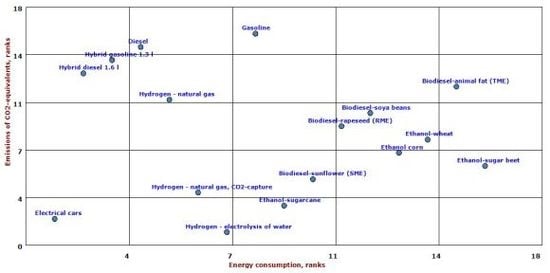
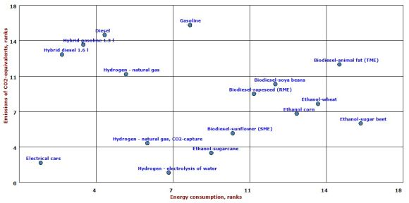
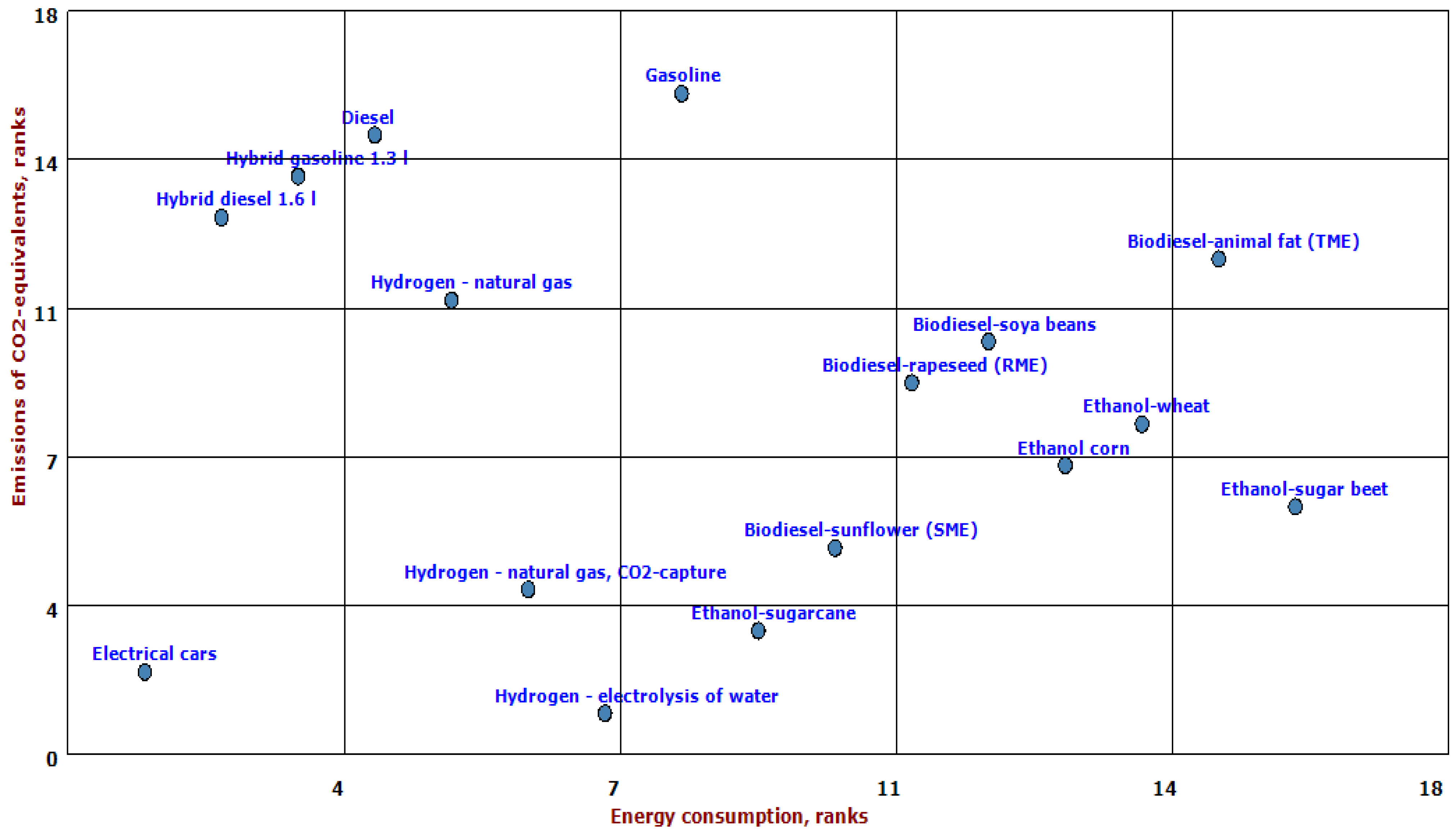
We will perform three statistical tests on the independence between ranks on energy consumption and ranks on emissions. The null hypothesis in all tests is that the ranks are distributed independently of each other. If that is the case, a fuel with a favourable rank on energy consumption is not likely to have a favourable rank on emissions. This means that knowing a fuels rank on energy consumption is not instrumental in predicting its rank on emissions. If this condition is fulfilled we have a rebound effect. This means that mitigation of an impact by switching to alternative fuels will increase other environmental impacts. This relation between ranks analyzed in this paper is visualized in
Figure 1, which shows the ranks for energy consumption versus ranks for emissions of CO
2-equivalents.
Figure 1.
Favourable vs. unfavourable ranks on energy consumption and greenhouse gas emissions.
Figure 1.
Favourable vs. unfavourable ranks on energy consumption and greenhouse gas emissions.
If the same fuel ranked favourably on both, we would expect the ranks to be the same. In that case, all points would be lying on a straight line increasing to the right with a regression coefficient of 1 and a R2 of 1. The measure R2 tells us how much of the variation in one rank is explained by variation in the other, and a value of 1 means that they are perfectly predicting each other. R2 varies between 0 (no relation) and 1 (perfect relation).
Those fuels that are more favourable on both impacts in
Figure 1 would be in the lower left corner of the figure. These are fuels with low ranks on energy
and low ranks on greenhouse gas emissions. Only electrical cars are in the lower far left corner, although hydrogen fuel produced with renewable energy or produced with CO
2-capture also comes out better to some extent than other fuels when we consider ranks on both impacts simultaneously.
If all fuels would consistently score favourable on one indicator and
unfavourable on another, all points would still lie on a straight line, but this line would be
decreasing to the right. The regression coefficient would be −1 and the
R2 would still be 1. This gives us a benchmark to assess how the ranks for energy consumption and emissions are related. The further away from 1 the actual
R2 coefficient in
Figure 1 is, the less the ranks are related to each other and the less chance there is for one particular fuel to be better than others for
both energy consumption and emissions.
In other words, the further the regression coefficient and the R2 is from the absolute value of 1, the less predictable the indicators are of each other and the more independent they vary. In figure 1, the regression coefficient in a linear bivariate regression model has a value of 0.103 while the value for R2 is 0.012. The F-test for the model yields a significance probability of 0.69 which is the probability of falsely rejecting a true null hypothesis. Since this probability is high, we choose to keep the null hypothesis of independent rank distributions. Consequently, we can conclude that the fuels’ scores on the two indicators are independent of each other. A fuel that has a favourable rank on energy consumption is more likely to have an unfavourable rank on emissions and vice versa. Exceptions to this are the electric car and hydrogen from natural gas with CO2-capture which has the low ranks on both. For all other fuels, their rank on energy consumption is not a good predictor for their rank on greenhouse gas emissions or vice versa.
We also note in
Figure 1 that conventional fuels and hybrids have relatively low energy consumption but high emissions of greenhouse gas emissions while biofuels, and especially ethanol fuels, have high energy consumption but low emissions. If the energy used in production of biofuels came from fossil energy sources, their overall mitigation of greenhouse gas emissions would be lessened.
The hypothesis of independence in the distribution of ranks can also be tested by a sign test [
33]. We assume the null hypothesis that the distribution of emission ranks are distributed independently from the distribution of energy ranks.
To test this hypothesis, we calculate the difference of the two ranks and test the distribution of these differences.
Table 17 shows the result. The median rank difference is 2. We will perform a test for difference in location of ranks which does not assume a normal distribution for the test statistic. This test is the sign test where the test statistic assumes the binomial probability distribution. The sign test is a non-parametric test for paired samples. In this case, we think of each fuel as a case in an observational study. We observe the same fuel twice, once for energy consumption and once for emissions of CO
2-equivalents. We calculate the difference in observation for each fuel using ranks as values.
We use the sign test here and not the Wilcoxon’s sign rank test. The reason for this is that the latter ranks the differences in observational values and performs tests on these ranks. Since we already use ranks as values in the test, we will use the sign test which only use the observational values as they are recorded without converting them to ranks.
Table 18 shows the result of the sign test. If the null hypothesis is true, the expected median difference in ranks should be zero. The test counts the number of times differences in fuel ranks is above zero, below zero and equal to zero. We let the fuels with zero difference in ranks count half in each direction. This gives us 6 rank differences above the median and 10 differences below. The test statistic for the two sided sign test is the minimum of these numbers which gives 6 as test statistic.
The critical c value in
Table 18 is the maximum value for the test statistic that will give rejection of the null hypothesis. The
c-value is calculated using 0.05 as a two-sided significance level. Any test statistic with a value equal to or higher than the critical c will lead to the null hypothesis
not being rejected.
Table 18 shows that the test statistic is higher than the critical value
c, therefore we do not reject the null hypothesis. The probability value for the test statistic in
Table 18 is calculated using the binomial distribution with values 16 for total number of trials, 6 for trials with success and 0.5 as probability for success in each trial. The calculated p-value is two-sided and is the cumulative probability value from the binomial distribution. We see from
Table 18 that the calculated p-value for the test statistics is greater than the significance level which leads to the same conclusion as with the critical value
c: The null hypothesis is
not rejected.
Table 17.
Difference of ranks calculated for the runs test.
Table 17.
Difference of ranks calculated for the runs test.
| Estimate | Energy | CO2-equiv. | Diff. |
|---|
| Biodiesel-animal fat (TME) | 15 | 12 | 3 |
| Biodiesel-rapeseed (RME) | 11 | 9 | 2 |
| Biodiesel-soya beans | 12 | 10 | 2 |
| Biodiesel-sunflower (SME) | 10 | 5 | 5 |
| Diesel | 4 | 15 | −11 |
| Electrical cars | 1 | 2 | −1 |
| Ethanol corn | 13 | 7 | 6 |
| Ethanol-sugar beet | 16 | 6 | 10 |
| Ethanol-sugarcane | 9 | 3 | 6 |
| Ethanol-wheat | 14 | 8 | 6 |
| Gasoline | 8 | 16 | −8 |
| Hybrid diesel 1.6 L | 2 | 13 | −11 |
| Hybrid gasoline 1.3 L | 3 | 14 | −11 |
| Hydrogen-electrolysis of water | 7 | 1 | 6 |
| Hydrogen-natural gas | 5 | 11 | −6 |
| Hydrogen-natural gas, CO2-capture | 6 | 4 | 2 |
Table 18.
Test results for sign test of difference in fuel ranks on energy consumption and greenhouse gas emissions.
Table 18.
Test results for sign test of difference in fuel ranks on energy consumption and greenhouse gas emissions.
| Results | Values |
|---|
| Number of observations | 16 |
| Number of observations < 0 | 6 |
| Number of observations > 0 | 10 |
| Number of observations = 0 | 0 |
| Significance level | 0.05 |
| Critical value for test statistics | 4 |
| Test statistic | 6 |
| p-value for test statistic | 0.4545 |
The result from the sign test points in the same direction as
Figure 1: the ranks are distributed independently of each other. This shows us that fuels which have favourable ranks on one impact will not tend to have the same favourable ranks on the other impact. Therefore, we can conclude that we have trade-off effects between energy consumption and greenhouse gas emissions, mitigation of one impact will most likely lead to an increase in another impact.
9. Conclusions
There is one fuel that scores better than any other fuels on any indicator. This is electricity. The trouble with this fuel is that electric cars in countries other than Norway would not have the same performance, since electricity in Norway is produced almost exclusively from hydropower. If all cars in Norway were to run on electricity, the capacity for hydroelectricity would also have to be increased many times. This simply might not be feasible. Also, electric cars of the 2010 vintage have a limited range, which means they are currently not real alternatives to conventional fuels. The figures in this article for electric cars must therefore be interpreted as indicative of the potential for electricity from renewable sources in the long run.
We started this paper by asking whether there were any trade-offs between energy use and greenhouse gas emissions from passenger car transport, or whether such a switch will only shift problems from one energy chain or from one impact to the other and thus offer no real mitigation. The answer must be that there is no substantial mitigation offered by alternative fuels and drivetrains, with the exception of electricity from hydropower. Electric cars have the potential for real mitigation, but only if their electricity comes from renewable sources. Hydrogen from natural gas with CO2-capture comes out better than most other fuels, though there are fuels with lower energy consumption but higher emissions. The same can be said for hydrogen from electrolysis of water with electricity from renewable energy. The problem with these hydrogen alternatives is that they are not implemented on a large scale. All other fuels and drivetrains discussed offer mitigation of one impact only through increasing another impact. There seems to be a trade-off effect that suggests that the requirements for sustainable transport can only be achieved through lower mobility with passenger cars.


